Chapter 8

Electroweak Unification

In Chapter 6, we listed the dream particles only dreamed of by ancient atomists in Fig. 5 of Chapter 6. In this chapter, we discuss the aspects related to the chiral property of these particles, especially how the weak and electromagnetic forces are unified (“electroweak”) in the Standard Model (SM) and in particular (1) how the SM fermions remain light, (2) the mystery of the light Higgs boson mass, and (3) possible unification of the SM into a grand unified theory (GUT) with the chiral property intact.

Weak interaction phenomena, known since Henri Becquerel (1852–1908) accidentally discovered that uranium salts spontaneously emit a penetrating radiation in 1896, have been completely understood in the second half of the 20th century. At length scales larger than 10⁻¹⁶ cm, the reality of quarks as discussed in Chapter 7 is of prime importance in ordering the jigsaw puzzle of elementary particles into Fig. 5 of Chapter 6. Particle physicists call this established model the SM of particle physics. All the fundamental particles in the SM are given in Fig. 5 of Chapter 6, the heart of atomists’ dream since the ancient Greeks. Here, we also include the story that finally established “how they pull or push each other”, the so-called interactions of elementary particles.

We study the universe and particles in it only after some point where we can reliably calculate the numbers. We are not philosophers, and do not question the creation of the universe as religious priests do. So, we are the evolutionists until the end of this chapter. Only if we can calculate numbers from first principles can we confidently talk about them as scientific knowledge.

Soon after the creation of the universe, the universe’s temperature was low enough (compared to GUT scale) such that calculations based on the SM have been possible. The time after the beginning of this expansion era was 10⁻¹² second. At that time, the universe was extremely hot with the temperature ten thousand trillion degrees Celsius. All the SM particles were moving with light velocity then. As the universe cools, the most massive particles lose the kinetic energy and are almost at rest in the comoving sphere of the universe. In a sense, it is similar to cooling oxtail soup. When one boils oxtail soup, mutton fat get dissolved in water at high temperature, but it get aggregated into white solids when the temperature is lowered. A similar phenomenon occurs for elementary particles, but with the governing laws of particle physics. Below a certain temperature, usually measured by the energy unit of eV (by particle physicists) that is roughly 10,000 Celsius, particles of mass of that temperature cease to move with light velocity. They become annihilated and leave no trace to the observers coming at a later time in the universe. We humans coming in 14 billion years later with the tool box, the SM kit, cannot know how these very heavy particles acted in the beginning of the universe. The question to answer is, “Which particles are here and now?” or, “Which particles are allowed to move with the light velocity at the time of 10⁻¹² second?” We know what particles are here and now; they are listed in Fig. 5 of Chapter 6. But, to answer the second question, there must be a knowledge of physics applicable at the time 10⁻¹² second. This problem may be related to the gauge hierarchy problem. The beta decay Becquerel observed had originated due to the so-called charged current (CC) weak interaction.

At this stage, we ask, “Which particles remain moving with light velocity?” In Fig. 1, we show L and R with thick arrows, denoting the spin angular momentum direction. Let us get an idea of how large the angular momentum will be if it were an orbital angular momentum which is proportional to the product of the rotating arm (horizontal small arrow) and the velocity of the rotating point. If the rotating arm is zero, the orbital angular momentum is zero. If a particle moves with light velocity and has a non-vanishing angular momentum that has three components, two components of angular momentum must be perpendicular to the propagating direction i.e. in the (xy)-plane or equivalently L or R. If one looks at the propagating direction, i.e. from the bottom of Fig. 1, L has the counterclockwise rotation (so −1 in the right-hand coordinate system) and R has the clockwise rotation (so +1 in the right-hand coordinate system). We obtain this conclusion because if it has mass, then its velocity must be smaller than the velocity of light and we can change the angular momentum into any direction off the (xy)-plane by changing its propagation velocity. But, for particles always moving with light velocity, the only direction is in the perpendicular direction. We name this helicity, from a helical orbital motion when propagating in the direction. Another word we use is polarisation. The best example is light which has two polarisations. Massless particles having angular momentum, for the spin angular momentum, have only two transverse polarisations. In this sense, the spin-2 graviton has two helicities, +2 and −2.

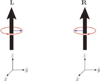
Figure 1: Rotating senses of L and R used in the text.

In 1957, 1 year after the discovery of parity violation in weak interactions, the “V–A” CC weak interaction was suggested by the “V–A” quartet, Marshak, Sudarshan, Feynman, and Gell-Mann. In the SM, the “V–A” CC weak interaction was suggested by Steven Weinberg by assigning the electron-type neutrino and L-handed electron of Fig. 5 of Chapter 6 in the same way in weak interactions as a doublet (ν_eL, e_L). In Fig. 1, the thick arrows denote this setup, L denoting the counterclockwise rotation and R denoting the clockwise rotation. (ν_e)_L and (e)_L in Fig. 5 of Chapter 6 interact with the W^± boson exactly in the same way. The bullet electron of Fig. 5 of Chapter 6 never interacts with W^±. Realisation of this simple fact was seriously applied in GUTs and extended GUTs by Howard Georgi, proposing the survival hypothesis on the masses. It is a hypothesis similar to conjectures if one cannot be certain of choosing one category among various possibilities. There are many ifs on the fundamentals on theories. One obvious one in particle physics like axioms in mathematics is gauge symmetry, which was discussed in Chapter 7. If we add many more decorations in addition to gauge symmetry such as discrete symmetries and global symmetries, particle theory can give almost infinite possibilities.

The survival hypothesis proposes that any pair with both L and R with the same gauge charge obtains mass at the temperature in consideration, i.e. at 10¹⁶ degrees Celsius, as mutton fat aggregates at some cold temperature. If there is no matching, then it is massless. Neutrinos with L-handedness only in Fig. 5 of Chapter 6 do not find their R-handed counterparts and remain massless at 10¹⁶ degrees Celsius. For electrons, the L-handed electron finds the R-handed one (bullet symbol), but their gauge charges are different; it is not a perfect matching. So, both L-handed and R-handed electrons remain massless at 10¹⁶ degrees Celsius or at 10¹² eV in terms of energy scale. In this way, the SM particles remain massless even if the temperature is lowered to below 10¹² eV. To reiterate, the first people to suggest this result, even if not spoken in this manner, were the “V–A” quartet of 1957.

When both chiralities L and R have otherwise the same quantum numbers, they combine to form a Dirac mass term at the ambient temperature, i.e. at 10¹⁶ degrees Centigrade. Without such matching, the states remain massless. This is called the “survival hypothesis”. Neutrinos with only an L component remain massless, as do electrons where the L and R components have different SU(2) assignments; all these states remain massless as the temperature falls below 10¹⁶ degree Celsius or equivalently 10¹² eV. This protection of light chiral states was first suggested in the (V − A) theory of 1958.

For spin-0 particles, chirality cannot be defined because there is no spin for chirality to be defined. The first guess on their mass is therefore very heavy. For a spin-0 particle to travel with light velocity like transversely polarised gauge bosons, its mass must be zero. In Fig. 1, its direction must be in the propagation direction ± since it should not carry an angular momentum. But, a natural mass of spin-0 particle is non-zero.

Mutton fat aggregation can be postponed by stirring mutton fat melted in water. fermions with both L- and R-handedness with perfect matching can be stirred with extra conditions, i.e. with more symmetries, such that they survive as massless particles below a temperature of 10¹² eV. Spin-1 gauge bosons are massless because of the gauge symmetry. But, spin-0 scalars are massive.

At this time of temperature 2.7° K, the SM particles are very heavy as shown in Fig. 3 of Chapter 6, with a top quark mass of 173 GeV, which is about million-billion times the current temperature. Even 2.7° is so low compared to the initial temperature at the time of universe creation that the SM particles in the end obtain mass. Looking at Fig. 5 of Chapter 6, there are three questions with one each for particles in the same circular band. First as, the Higgs particle in the centre is related, “How do the SM particles obtain mass?” Second, for the spin-1 particles in the middle, in addition to the gluons discussed in Chapter 7 there is a question, “Why are there just four particles for the mediation of weak and electromagnetic interactions?” Third, for the fermions in the outer band, “Why are there 45 chiral fermions?”

The answer to the second question was the finding of the electroweak gauge symmetry SU(2)×U(1) by Sheldon Glashow (1932–) in 1960. An earlier attempt had been made by Glashow’s PhD adviser, Julian Schwinger (1918–1994) in 1957, but he did not have the correct experimental information about weak interactions and so followed a false trail. Sometimes, it is said that it is the unification of weak and electromagnetic forces in the sense that both must be treated in the same gauge symmetry principle. Since Maxwell’s electromagnetism of 1865, it was the first and successful unification pulling weak interactions in this arena. But, the SM included two coupling parameters α₂ and α₁ for the factors SU(2) and U(1), respectively. Unification with just one coupling constant was (unsuccessfully) attempted over a decade later, under the name of grand unified theories (GUTs) of all elementary particle forces, except gravity.

Giving mass to the W^± and the Z⁰ proved to be a more difficult problem. In 1960, Glashow wrote that the masses were a “stumbling block” which must be temporarily ignored in his paper, which discovered the electroweak gauge structure of the standard model. This provides an interesting example of solving one crucial problem while deliberately delaying the solution of another.

With the W^± and the Z⁰ masses, weak interactions of proton, neutron, muon, and other light fermions are given by Fermi’s constant G_F for the weak CC and another coupling for the weak neutral current (NC). Usually, these two couplings are discussed in terms of G_F and the weak mixing angle sin² θ_W . So, the first experimental confirmations were centred on fitting all the weak NC experiments in terms of one parameter: the weak mixing angle sin² θ_W .

The weak NC was first discovered by the Gargamelle bubble chamber at CERN in 1973. A final hurdle to checking the gauge structure of SU(2)×U(1) was to discover the parity-violating coupling of Z⁰ to electrons. Note that one aspect of weak interaction is parity violation. This predicted from the eeZ coupling an optical rotation of polarised light traversing certain gases, and in experiments carried out at Seattle and Oxford such a rotation could not be successfully detected. Until 1978, these atomic experiments cast serious doubt on the model.

In 1978, however, a more direct measurement of the eeZ coupling, i.e. the weak NC effect, was completed, involving scattering of polarised electrons off deuterium at SLAC by Charles Prescott (1938–) and Richard Taylor (1929–2018). This brilliant experiment, which detected an effect order of magnitude smaller than the dominant electromagnetic contribution, convinced the particle theory community that the SM is correct after the report by Taylor at the ICHEP 1978 conference in Tokyo, Japan. In fact, in the evening of the closing day of ICHEP 1978, the Japanese National TV broadcasted a documentary on the story of the SM.

With the value 0.233 for sin² θ_W reported a year later at the 1979 International Conference on Neutrinos held at Bergen, Norway, the Z⁰ mass was predicted to be 91 GeV. The spin-1 gauge boson Z⁰ with this mass was in fact produced by the Proton–Antiproton Collider at CERN in 1983, which was reported by two experimental groups at CERN, the UA1 group led by Carlo Rubbia (1934–) and the UA2 group. This discovery confirmed the SM experimentally, and the precision NC data on the weak mixing angle 0.233 determined in this period are still correct compared to a more accurate value determined by the recent experiments at the Large Hadron Collider (LHC) of CERN. The gauge boson W^± for the source of the weak CC was discovered by the UA1 and UA2 groups of CERN, also in 1983.

Glashow’s dilemma, “stumbling block”, for the mass of Z⁰ and W^± is the heart of the first problem at the centre of Fig. 5 of Chapter 6. Glashow’s “stumbling block” was removed by the so-called Higgs mechanism, which was worked out in 1964 by Francois Englert (1932–), Robert Brout (1928–2011), Peter Higgs (1929–), Gerald Guralnik (1936–2014), Carl Hagen (1937–), and Thomas Kibble (1932–2016).

The Higgs mechanism was correctly used in the SM gauge group SU(2) × U(1). With gauge symmetry, i.e. with massless particles, all gauge bosons have the transverse polarisation as mentioned earlier. Helicity is the rotational sense measured in the direction of propagation: the sense L in Fig. 1 is denoted by −1 and the sense R is denoted by +1. A natural mass of spin-0 particle is non-zero. For this spin-0 to combine with the transverse gauge boson, it must have exactly the same property except the spin. First, it is pseudoscalar, having the same gauge transformation property. Second, its direction must be in the propagation direction since it should not carry an angular momentum. Third, it must travel with light velocity to say “Hello” to the transverse gauge boson, moving together in the same direction with light velocity. To travel with light velocity, its mass should be zero. But, we said above that a natural mass of spin-0 particle is non-zero. This condition is evaded if a global symmetry in question is spontaneously broken.

To give mass to massless gauge boson, we need polarisation to the longitudinal direction (the forward or backward direction of propagation) in addition to the two transverse degrees of spin-1 gauge boson. Spin-0 pseudoscalars provide these longitudinal degrees. For both gauge bosons W^± and Z⁰ to be massive, we must provide three pseudoscalars. But, except the spin difference, all the other properties must be the same. Since these gauge bosons transform non-trivially at least under the SU(2) transformation, we need some pseudoscalars transforming non-trivially under the SU(2) transformation. Steven Weinberg and Abdus Salam suggested that two complex scalars, or four real scalars, are grouped into one complex doublet.

In the interpretation of quantum mechanics by Max Born and Chen Ning Yang in Chapter 5, quantum mechanics is phase mechanics. We are considering spin-1 gauge boson and spin-0 scalar. The gauge transformation on the scalars appear in the phase. So, three scalars appear in the phase, whose number 3 matches the three gauge bosons in SU(2). (As discussed in Chapter 7, there are N² − 1 gauge bosons for an SU(N) gauge theory.) Out of the four scalars we introduced, where did the remaining one go? It must belong to the real coefficient of the exponential factor. Counting the number of scalars in this way is the unitary gauge since we used the unitary transformation. In this setup, the property of the remaining scalar is the property of vacuum or ground state, which is discovered in technical books as the vacuum expectation value (VEV). If a scalar field gets a VEV and breaks a symmetry, it is called “spontaneous symmetry breaking”.

The real scalar is called the Higgs boson and was finally discovered at CERN in 2012 with the mass value 125 GeV. This is the Higgs mechanism, which breaks the SU(2)×U(1) electroweak symmetry to only U(1) electromagnetic symmetry and thereby generates the mass of the W^± and Z⁰. Because we used only three pseudoscalars, we cannot make the remaining gauge boson massive as pointed out by Tom Kibble in 1966. This remaining gauge boson is a photon. A major advantage of the Higgs mechanism is that the theory preserves renormalisability proven first by Tiny Veltman (1931–) and Gerard ’t Hooft (1946–) and in a more understandable way by Ben Lee (1935–1977) and Jean Zinn-Justin (1943–), which puts the standard model on a footing with QED in that the quantum corrections can be consistently calculated with high accuracy.

From the non-relativistic condensed matter property, the essence of Higgs mechanism was known in the late 1950s to Yoichiro Nambu (1921–2015) and Phillip Anderson (1923–). The road toward the relativistic form of spontaneous symmetry breaking in particle physics, discussed in the above paragraph, was started by Jeffrey Goldstone (1933–) and discussed without local gauge symmetry by Goldstone, Weinberg, and Salam. Peter Higgs used the same form suggested by Goldstone but with the input of local gauge symmetry and found that there remains a physically observable real scalar.

Spontaneous symmetry breaking of gauge symmetries sometimes introduces magnetic monopoles via the so-called Kibble mechanism. At every space point, the VEV of a Higgs field can be assigned. If the VEV is the same everywhere, the effect is making some gauge bosons massive, just by counting which gauge boson obtains the longitudinal degree. In the four-dimensional space–time, we presented the instanton solution as the gauge field values in Chapter 7, as shown in Fig. 4. Now, we consider field values of the Higgs field. Suppose that an unbroken U(1) gauge theory results from spontaneous symmetry breaking. Consideration of U(1)_em by breaking the SM gauge group SU(2)×U(1) does not apply here because we have U(1) before and after the symmetry breaking. Transformation under U(1) is a circle, mathematically denoted as a sphere in one dimension S₁.

An interesting situation occurs when one creates an S₁ circle out of no circle. In general, the group space of non-abelian simple groups does not have S₁. We said that a quantum mechanical transformation is a phase, meaning on the surface of a unit sphere. In this sense, U(1) is sitting on a circle, i.e. the circumference of a two-dimensional sphere disk. The SU(2) instanton solution was sitting on S₃, the surface of a four-dimensional sphere. Since we want a localised particle, we consider the surface of three-dimensional sphere, i.e. S₂. Any simple group has SU(2) as a subgroup. So, SU(2) group directions can be put on the surface of a three dimensional ball. What will happen if this SU(2) gauge symmetry is broken to U(1) gauge symmetry? For an electric monopole, it is shown in Fig. 1 of Chapter 7. However, Maxwell’s equation does not introduce magnetic monopoles, i.e. the magnetic fields do not have ending sources. Can a magnetic monopole appear in case a simple group such as SU(2) breaks to produce a U(1) gauge theory? Yes, it happens because of the Kibble mechanism on the VEVs of Higgs fields in the universe as the universe cools down. It was discovered by ’t Hooft (1946–) and Alexander Polyakov (1945–), and the resulting monopole is called a ’t Hooft–Polyakov monopole.

The Higgs field has at least four real components such that three parameters can be in the phase, i.e. to associate with an SU(2) symmetry. Then, the VEVs of the Higgs field can have hedgehog-type directions as shown in Fig. 2(a). At the origin, the VEV is zero. Suppose we calculate the outgoing B fields as shown there. Indeed, ’t Hooft and Polyakov showed that there arises a B field proportional to 1/r² at a large radius r. There must be a magnetic monopole sitting at the origin. But, U(1) charges are counted by the flux since it is a gauge theory. Suppose we move topologically all B fields to a line as shown in Fig. 2(b). Then, the flux is calculated just on the small disk, and hence by the boundary (red dashed line in Fig. 2(b)) of the disk by the Stokes theorem. So, shifting the phase over a circle must give an identity, e^{i2π·integer} such that one can never see the outgoing flux experimentally. This gives the quantisation condition of the magnetic charge and depends on the VEVs of Higgs fields, i.e. how SU(2) is broken down to U(1). The magnetic monopole mass is of order (VEV)/e.

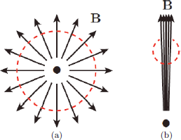
Figure 2: Magnetic monopole.

This has a far-reaching consequence in GUTs such as SU(5). SU(5) is broken to the SM containing U(1) factor and hence magnetic monopoles of mass around 10¹⁶–¹⁷ GeV should appear if the GUT is the one that nature chose. These heavy monopoles could never have led to our universe as pointed out by John Preskill (1953–). What should we do? Even though the flatness and isotropic problems are counted as the primary reasons now, the monopole problem was used as one motivation for the inflationary scenario by Alan Guth (1947–).

The third question related to the outermost particles of Fig. 5 of Chapter 6 is the flavour problem or the family problem. After obtaining order of hadrons in Chapter 7, it was determined that SU(3) flavour symmetry was established. But, hadrons with flavour SU(3) (or three quarks u, d, and s) were plagued with the apparently fatal problem of predicting strangeness-changing weak processes too large to agree with experiment. This problem was solved in 1970 by three Harvard physicists, GIM (Sheldon Glashow, John Iliopoulos (1940–), and Luciano Maiani (1941–)), who predicted the existence of a fourth flavour of quark, named charm c.¹ The charmed quark was dramatically discovered in the so-called 1974 November Revolution started by Samuel Ting (1936–). Since 1974, Gell-Mann’s mathematical quarks were established in the atomic world as a reality.

Two further flavours or quarks, bottom (b) and top (t), were subsequently discovered in 1977 and 1995, respectively, to accompany three families of charged leptons e⁻, μ⁻, τ⁻ and neutrinos ν_e, ν_μ, ν_τ. These are the 45 chiral fermions in the outermost ring in Fig. 5 of Chapter 6. In fact, the same number of families are needed to preserve renormalisability of the SM, as pointed out in 1972.

Three quark families are needed if time reversal symmetry in the SM is required to be broken just by the weak CC interactions. Time reversal is like playing a video of a movie backward. In the SM, time reversal symmetry is like changing a particle to its antiparticle at the opposite point with respect to an origin. It is called CP symmetry. Talking in terms of CP is better for experimentalists since it is difficult for them to make a device with time running in the backward direction. The three-family condition in the SM for the weak CP violation was found by two Japanese physicists Mokoto Kobayashi (1944–) and Toshihide Maskawa (1940–). So far since 2006, experimentalists did not find any hint that we require any additional source for the weak CP violation in particle physics.

Talking in terms of CCs of three families is equivalent to discussing six quarks (three quarks with charge and three quarks with ) with L-handed chirality only. For equally charged quarks, for example u, c, t, quark mixing is possible. The possibility of quark mixing was found by Nicola Cabibbo. General quark mixing relevant for the weak CC interaction needs a 3 × 3 unitary matrix. The most general and physically relevant 3 × 3 unitary matrix is parametrised by three real angles and a phase, which is called the CKM matrix in which the phase is called the KM phase for which Kobayashi and Maskawa were credited by the Nobel Committee in 2008. Lincoln Wolfenstein (1923–2015) wrote a CKM matrix in 1983 such that it is easily usable by experimentalists, and most hadronic data were analysed using this form. This approximate form is correct for entries in the matrix bigger than 0.01. In 1985, Swedish Cecilia Jarlskog (1941–) noted a simple number J which is the same in any CKM parametrisation. The reason the Nobel Committee credited Kobayashi and Maskawa was because all hadronic experiments converged to giving J at a value little bit smaller than 0.0001. So, there was a need to analyse data with CKM parametrisations which are exactly unitary.

The corresponding leptonic sector also carries three families. There are both chiralities (L and R) of electron, muon, and tau. As already mentioned in an earlier Chapter 5 and Fig. 5 of Chapter 6, the accompanying neutrinos, electron-type neutrino ν_e, muon-type neutrino ν_μ, and tau-type neutrino ν_τ come only with one chirality L. Introduction of neutrinos in 1930 by Wolfgang Pauli (1900–1958) for nuclear β-decay was for neutrino mass, of the order of nucleon mass, but it was before knowing anything about the stories of the “V–A” quartet. In the SM, therefore, neutrino masses are zero at the renormalisable level.

Pauli’s bold hypothesis was incorporated into Fermi’s theory of weak interactions in 1934 and in all further such theories, although the neutrino was not directly detected until 1956 by Frederick Reines (1918–1998) and Clyde Cowan, (1919–1974) at the Savannah River nuclear reactor in South Carolina. That was what we now call the electron-type antineutrino. In 1962, Leon Lederman (1922–2018), Melvin Schwartz (1932–2006), and Jack Steinberger (1921–) showed experimentally that there were at least two different flavours of neutrino. Now, we have evidence for three, ν_e, ν_μ, ν_τ , completing the required 45 chiral fields of Fig. 5 of Chapter 6.

In the SM and also in an SU(5) GUT, the neutrinos were assumed to be massless and represented by L-handed Weyl spinors. The massless neutrino would travel at the speed of light and have a definite helicity as mentioned above, i.e. only L-handed according to experiments on β-decay based on CCs.

Everything changed in 1998 when at the Super-Kamiokande experiment in Japan it was convincingly shown that neutrinos entering the atmosphere changed flavour, or oscillated, possible only with a non-zero mass. Many more experiments have confirmed this and thus there is a non-trivial 3 × 3 mixing matrix for the three neutrino types as the CKM matrix in the quark sector, which has spawned a large field of research, especially as it is the only well-established deviation from the original minimal standard model.

In the quark sector, hadron masses come in the discussion of mixing experiments at low energy. In most neutrino experiments, neutrinos travel with almost light velocity and the kinetic energy is more important, and hence mixing experiments use the energy of neutrinos. A correct formula for the neutrino oscillation was given in 1957 by Russian Physicist Bruno Pontecorvo (1913–1993) for an electron-type neutrino to its anti-neutrino because any other neutrino was not known at that time. For neutrinos carrying no electric charge, neutrino and antineutrino oscillation is possible and hence in general a 6×6 mixing matrix can be considered. But, to discuss it in parallel with the CKM matrix, we neglect the small neutrino–anti-neutrino oscillation, and consider the 3 × 3 mixing matrix, following Ziro Maki, Masami Nakagawa, and Shoichi Sakata (1911–1970), which can be called the MNS matrix. Most physicists, however, call it the PMNS matrix, which has three mixing angles and three CP-violating phases. It is irresistible to compare this PMNS matrix with the CKM matrix. The CKM matrix has one CP-violating phase. Two of the three real angles are very small and the largest, the Cabibbo angle, is only about 13°. In the PMNS matrix, by contrast, the mixing angles are much bigger, one being close to maximal (45°), one about 34°, and the smallest being 9°.

This qualitative difference means that in any theory of flavour symmetry, the quarks and leptons must belong to different representations of a discrete flavour group. Another difference is that the neutrino masses are a million times smaller than those for any of the charged leptons and quarks.

Non-zero neutrino masses, in a world with the SM fields only, require non-renormalisable interactions of the SM fields. How these interactions appear depends on the details of a model. Steven Weinberg considered, in effect, a non-renormalisable form for the quark mass matrix in 1977. For a 2 × 2 matrix, one diagonal element was very heavy, say M, and two off-diagonal elements were small, say v, and the remaining diagonal element was zero. Because of the invariance of the determinant, two eigenvalues are approximately given, M and v²/M, which is the basis of the seesaw mechanism that if M goes up, the other goes down. Here, v is considered to be a VEV of some scalar field σ and 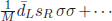is an effective non-renormalisable interaction. This non-renormalisable quark interaction preserves the baryon number.

The most elegant explanation of the tininess of the neutrino masses is the so-called seesaw mechanism, which invokes at least two, usually three, right-handed super-heavy neutrinos as suggested in 1977 by Peter Minkowski. Note here that neutrinos in the SM are only L-handed and the non-renormalisable interactions for masses must be of the Majorana type, breaking lepton number. As far as the seesaw mechanism is concerned, it is the same as above. But, since the non-renormalisable interactions break the lepton number, that breaking must be taken into account. It is done by introducing heavy SU(2)×U(1) singlet neutrinos. So, to confirm, the seesaw mechanism is rendered challenging by the heaviness of the right-handed neutrinos, if they exist. If there were three light neutrinos, one needs three heavy neutrinos in the most straightforward generalisation.

There are two gauge coupling constants in the SM, and hence it is not a true unification of coupling constants. We discussed the parameter, the weak mixing angle put in by hand in the SM. To have one gauge coupling constant, grand unified theories (GUTs) have been considered. In GUTs, therefore, the weak mixing angle sin² θ_W is determined. We recall that the experimentally determined value is close to 0.233 at the electroweak scale.

As Howard Georgi and Sheldon Glashow did in SU(5), we can use all L-handed ones, just replacing R-handed ones (the bullets) of Fig. 5 of Chapter 6 with L-handed antiparticles. This is called a chiral representation since we used only one chirality L. This is the magic of quantum field theory (QFT). Georgi and Glashow played the part of magicians. A trick in QFT is that a quantum field defined for a species of a particle can create a particle and can also annihilate its antiparticle. For particles, the opposite chirality is used for antiparticles. Whether we use a quantum field of particle or that of antiparticle, the same is achieved if we wanted to create a particle. If we use the quantum field of the particle, we use the creation operator. On the contrary if we use the quantum field of the antiparticle, then we use the annihilation operator. Another magical effect of QFT is that all electrons created by the electron quantum field are identical, or indistinguishable, in the whole universe.

The 15 chiral fields in one family of Fig. 5 of Chapter 6 are grouped to five and 10 groups such that all electromagnetic charges in each group sum up to zero. That is possible with gauge group SU(5). The collection of five is electron-type neutrino, which is L-handed, L-handed electron, and three colours of anti-d quark that are all L-handed. In Fig. 5 of Chapter 6, we used both L-handed particles and R-handed particles, but Georgi and Glashow used a chiral representation for helicity L. Then, all bulleted ones are replaced by triangles with opposite charges, both for the electromagnetic and colour charges. Thus, the electromagnetic charge of anti-d quark is and the sum of electromagnetic charges for the members of the group is which is zero. For the sum of colour charges, we have to consider two numbers like the third component of isospin and the hypercharge described in Chapter 7, but this time for the colour gauge group SU(3)_colour. For a triplet or an antitriplet of quarks, sum of colour sisospin is zero, and so it is for colour hypercharge. This group of five is the fundamental representation of group SU(5). The essence of the SU(5) GUT is contained in this collection of five particles.

Charge quantisation is achieved. From the sum of the electromagnetic charges, the electromagnetic charge of d quark was determined above as which determines the electromagnetic charge of u quark as So, the charge of proton, i.e. the electromagnetic charge of uud, is +1. GUTs solve a long-standing puzzle that the sum of electron and proton charges is zero. If the universe is full of hydrogen atoms, the total charge of the universe is zero. All heavier elements can be manufactured from hydrogen atoms and neutrons which are electrically neutral.

The weak mixing angle sin² θ_W is determined. Basically, the weak mixing angle is given by the ratio of two coupling constants in the SM. Since GUTs have one coupling constant, the ratio is fixed. The SU(5) GUT determines the weak mixing angle as But, this is the case when the unification is still valid. If the GUT group is broken down to the SM gauge group, say at a 10¹⁶-GeV energy scale or at the length scale of 10⁻³⁰ cm, the coupling strengths at larger length scales are as shown in Fig. 3. The QCD coupling is shown as the red curve. The SU(2) and U(1) coupling constants are shown as black curves, and the weak mixing angle is a ratio of these two curves. at the GUT scale evolves to a smaller value, ending up close to 0.233 at the electroweak scale. This is one great success of GUTs.

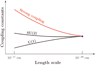
Figure 3: Magnitudes of coupling constants.

Figure 3 does not explain why we stopped the figure at the length scale of 10⁻¹⁷ cm. Several high-energy accelerators, including Tevatron of Fermilab and LHC of CERN, confirmed that the value of the strong coupling at 10⁻¹⁷ cm is about 0.118. If we continue the red curve to larger length scales, we notice that it is O(1) at the length scale of 10⁻¹⁴ cm. In fact, strong interactions at low energy are determined by physics at the 10⁻¹⁴ cm, and we do not discuss physics in terms of quarks for length scales larger than the proton size. This can be applied to electroweak physics if some gauge coupling constant becomes O(1) at the scale 10⁻¹⁸ cm. The corresponding curve is not shown in Fig. 3. This kind of idea was called “technicolour” in the late 1970s by Leonard Susskind (1940–) and Steven Weinberg, which is a suggestion for generating the hierarchy of two scales, 10⁻³⁰ and 10⁻¹⁷ cm. This method uses dimensionless coupling constant to generate the length scale (or mass scale) when couplings become O(1) under the name of dimensional transmutation. This method, however, does not give the observed quark and lepton masses, and failed in the flavour problem.

To give quark and lepton masses correctly, the Yukawa couplings by Higgs field is definitely needed. In fact, the Higgs boson was discovered at the LHC of CERN in 2012.

Before listing open questions, we comment on the attempts to understand the hierarchy problem. Since the hierarchy is so huge, of order 10¹⁶ in terms of ratio of scales, exponential factor was preferred. In Chapter 6, supersymmetry and superstring were discussed in this regard.

One attempt was introducing some kind of curvature in higher dimensions. If the curvature is extremely large for some internal dimensions and zero for our four-dimensional universe, there may arise an exponential factor. This idea was proposed with warped space by Lisa Randall (1962–) and Raman Sundrum (1964–). The exponential factor is introduced in the ansatz on the metric as e^−k|y|, where y is roughly the size of the internal space. Newton’s constant for gravity G_Newton is discussed in terms of the Planck mass, M_P = = 2.43 × 10¹⁸ GeV in the natural unit. Its inverse may be taken as the Planck length 10⁻³² cm. The scale for the internal space may be taken as a string length 10⁻³² cm, or something else. An exponential factor of 10⁻¹⁶ is obtained from e^−k|y| for Who fixes this value of 36.84? Is this another tuning or not? Suppose that we change it to 35. Then, the exponential factor is 6.3 × 10⁻¹⁶, corresponding to Z⁰ boson mass of 573 GeV. Suppose that we change it to 40. Then, the exponential factor is 0.0042×10⁻¹⁶, corresponding to Z⁰ boson mass of 0.38 GeV. It seems that there is no a priori condition fixing this value of the internal space of It belongs to God’s design on the size of internal space.

Another attempt at introducing an exponential factor was a confining force of Weinberg and Susskind under the name of technicolour. But, it failed miserably in flavour physics. For flavour physics, scalars are assigned chirality by the N = 1 supersymmetry. The supersymmetry idea needs a confining force again to break super-symmetry. Here, the problem was how to generate the scale 246 GeV for the VEV of Higgs doublet. The best idea is again the dimensional transmutation mentioned along with Fig. 3. If there is a new confining force in the hidden sector, it is required to confine above 10¹⁰ GeV as shown in Fig. 4. This picture is drawn without taking into account the gravitational interaction mentioned in Chapter 6. If a scalar develops a VEV at 5 × 10¹⁰ GeV, the effect of gravity will induce the superpartner masses of order (5 × 10¹⁰)²/2.43 × 10¹⁸ GeV, which is about 1,000 GeV. If a scalar develops a VEV at 10¹¹ GeV, the effect of gravity will induce the superpartner masses of order 4,000 GeV. Realising this kind of hierarchy solution with supersymmetry is not ruled out yet and even higher energy data are needed. The coupling at the black bullet determines all physics scales below it. Who determined that value of α_New? It is determined in relation to the other couplings of the SM in some ultraviolet completed theories. In this sense, this idea belongs to Darwinism.

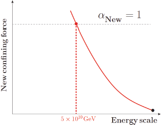
Figure 4: A new confining force from the hidden sector.

In the last two paragraphs, we showed two examples of possible gauge hierarchy solutions. It seems that the theory may lie midway between Darwin and Shakespeare.

1 S. L. Glashow, J. Iliopoulos, and L. Maiani, Weak Interactions with Lepton-Hadron Symmetry, Phys. Rev. D 2, 1285 (1970).