3
Model-Based PID and Resonant Controller Design
3.1 Introduction
The models used in the design of PID controllers are limited to two particular types. One is a first order model while the other is a second order model. If the plant dynamics yield a higher order model, an approximation is often involved to obtain a first order or a second order model so that a PID controller can be designed using a model based approach.
When using model based design methods, a desired closed-loop performance specification is required before commencing. The desired performance is chosen in terms of the locations of the desired closed-loop poles, which reflect the closed- loop response time to reference change and disturbance rejection or in the frequency domain the bandwidth of the desired closed- loop control system. The desired closed-loop performance is often adjusted several times using closed-loop simulation and experimental validation before the designer finds the suitable closed-loop performance.
3.2 PI Controller Design
To design a PI controller, a first order model is used. Although the first order dynamics is the basic unit to form a system, it can also be used to describe a number of commonly encountered physical systems, such as the dynamic relationship between motor torque and angular velocity in the motor control problem, and fluid in-flow rate and fluid level in a fluid vessel control problem.
3.2.1 Desired Closed-loop Performance Specification
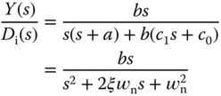
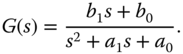
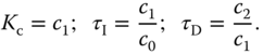
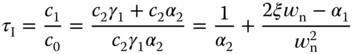
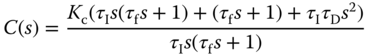
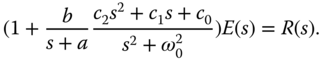
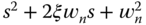
In the model-based design, a desired closed-loop performance is required to be specified. In the PI controller case, a second order transfer function is used in the specification,
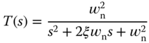
where  and
and  are the natural frequency and damping coefficient for the second order transfer function. These are the free parameters to be selected by the designer as the desired performance specification.
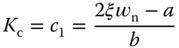
The parameter  is often chosen as 1 or 0.707. When
  , the poles of the desired closed-loop transfer function (3.1) are the solutions of the polynomial equation,
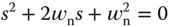
which are 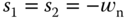 . Namely, we have two identical poles when
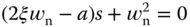
  . With the second choice of
  , the poles are a pair of complex conjugate numbers determined by
With the parameter  chosen (either 1 or 0.707), the natural frequency
  becomes a closed-loop performance parameter that the user specifies according to the desired closed-loop response requirement. In general, when
  is larger, the desired closed-loop response is faster. The parameter
  is directly related to the closed-loop response time and the band limit of the closed-loop system, which provide us with the guidelines on its selection. These two aspects are examined.
From the simulation of a step response (3.1) (see Figure 3.1), the response time is inversely proportional to the parameter  . Figure 3.1(a) shows that with the damping coefficient
  , the total step response time is about
  and with
  , as shown in Figure 3.1(b), the total step response time is about
  . There is another estimate of
  that can be used as a guideline for the designer. Here the parameter
  is related to the bandwidth of the desired closed-loop control system. For the desired closed-loop transfer function given by (3.1), when
  , it can be verified that
  at the frequency
  . Hence, with the special choice of the damping coefficient
  , the natural frequency
  is the bandwidth of the closed-loop system, which we can directly use for the closed-loop performance specification. With the choice of
  , the bandwidth of the closed-loop system is slightly smaller.
3.2.2 Model and Controller Structures
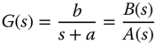
For the first order model, we assume that a first order time constant  and a steady state gain
  are known to form the Laplace transfer function,

Figure 3.1 Step response of the desired closed-loop transfer function. (a)  . (b)
. (b)  . Key: line (1)
  ; line (2)
  .
.
which can also be expressed in the pole–zero form,
where  and
and 
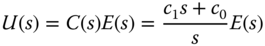
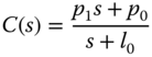
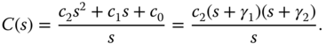
For a PI controller, its transfer function is given by
which can be written in the transfer function form,
where  and
and  . We will first find the coefficients
  and
and  based on the model (3.5), then convert these coefficients into the standard PI controller parameters
  and
and  .
.
The key to the solution of the PI controller parameters is to equate the desired closed-loop poles to the actual closed-loop poles. The locations of the closed-loop poles determine whether the closed-loop system is stable, the closed-loop response time, and the band limit of the closed-loop system.
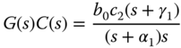
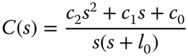
To this end, we calculate the actual closed-loop system using the design model (3.5) and the controller model (3.7) via the closed-loop transfer function

The closed-loop poles of the actual system are the solutions of the polynomial equation with respect to  :
:
Equation 3.9 is called the closed-loop characteristic equation. Since the model parameters  and
and  are given, the free parameters in (3.9) are the controller parameters
  and
and  . To find the controller parameters
  and
and  , the following polynomial equation is set:

where the left-hand side of the equation 3.10 is the polynomial that determines the actual closed-loop poles and the right-hand side is the polynomial that determines the desired closed-loop poles. By equating these two polynomials, the actual closed-loop poles are assigned to the desired closed-loop poles. This controller design technique is called pole assignment controller design.
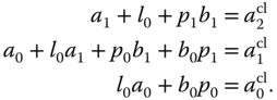
Now, we compare the coefficients of the polynomial equation 3.10 on both sides:


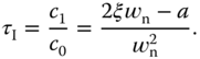
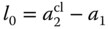
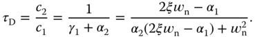
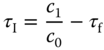
Solving (3.12) gives
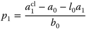
and solving (3.13) gives

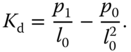
With the relationships between  ,
,  and
and  ,
,  (see Equation 3.7), we find the PI controller parameters as
3.2.3 Closed-loop Transfer Functions for Different Configurations
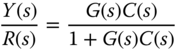
With the PI controller designed, now we study the closed-loop transfer functions for using the traditional PI controller configuration and the IP controller configuration.
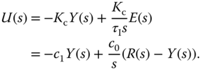
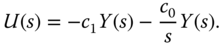
For the traditional PI controller configuration (see Figure 1.5), the Laplace transform of the control signal,  , is expressed as the function of feedback error signal
  using the relation
where  and
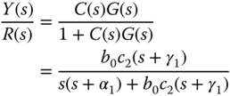
and 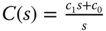 . The closed- loop transfer function between the reference signal
  and the output signal
  is then
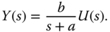
where  is the first order transfer function
  . By substituting the transfer functions of controller (
 ) and the plant transfer function
  into (3.20), we obtain the closed-loop transfer function for the PI control system using the traditional implementation:
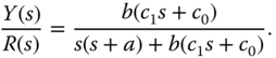
Note that the denominator of (3.21) is used in the design of the PI controller (see (3.10)), which is made equal to the desired closed-loop characteristic polynomial  . By substituting the controller parameters (see (3.14) and (3.15) and the desired closed-loop characteristic polynomial into (3.21), the closed-loop transfer function becomes:
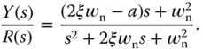
Using the traditional PI controller configuration, the actual closed-loop transfer function between the reference signal and the output is not equal to the desired closed-loop transfer function specified in the design (see  in (3.8)). Instead, there is a zero in the closed-loop transfer function at the location determined by the polynomial equation:
which is at 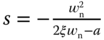 . The existence of this zero could cause some overshoot in the step response. One can verify that the closed-loop transfer function (3.22) has a bandwidth larger than
  for the choice of
  .
.
For the IP controller configuration (see Figure 1.7), the control signal is expressed as
The output signal  is expressed as
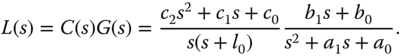
By substituting (3.24) into (3.25), we find the closed-loop transfer function for the alternative configuration as
By the design procedure, the denominator of this transfer function is  and the numerator
  , therefore the closed-loop transfer function is
which is equal to the desired closed-loop transfer function we specified in the performance specification (see (3.1)).
As for disturbance rejection and measurement noise attenuation, both PI control system configurations have the identical closed- loop transfer function because the structural change introduced in the alternative configuration is only related to how the reference signal is introduced in the feedback loop. We illustrate this point by calculating the closed-loop transfer function between input disturbance and the plant output.
Suppose that an input disturbance has a Laplace transform  and it enters the system at the position of plant input. In this case, the plant output is expressed as
To derive the closed-loop transfer function between the input disturbance and the plant output, we assume that the reference signal  so to concentrate on the disturbance rejection. When the reference signal
  , the control signals from both configurations (see (3.19) and (3.24)) become identical to the transform:
Substituting (3.29) into (3.28), we obtain the closed-loop transfer function between the input disturbance  and output
  as
as
where we have used the design equation in (3.10).
Note that there is a factor  in the numerator of the closed-loop transfer function. This factor ensures that the closed-loop control system will reject a step input disturbance without steady- state error. This point will be made clear through the examples in the following section.
3.2.4 Food for Thought
- Would you use a second order model to design a PI controller?
- If you found that the closed-loop response speed was too slow, would you decrease the parameter
 ?
? - Is it correct to say that the closed-loop bandwidth
 when the closed-loop system transfer function is characterized by
  if the damping coefficient
  ?
?
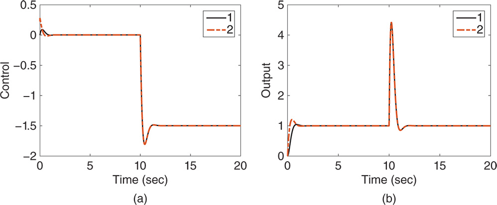
Figure 3.3 Closed-loop response of PI control system (Example 3.2). (a) Control signal. (b) Output response. Key: line (1) IP control system; line (2) PI control system.
- Would you be able to list three physical systems that can be described by a first order model?
- Has the IP controller configuration changed the characteristics of disturbance rejection when comparing with the original PI controller?
3.3 Model Based Design for PID Controllers
Second order models are used directly for the design of a PD or a PID controller. In addition, a first order plus delay model is approximated using a second order transfer function model, where the irrational transfer function  is approximated using a rational transfer function
  that is called first order Padé approximation. If the mathematical model is of higher order, then approximation is made to obtain a second order model in order for the PID controller design to be carried out.
3.3.1 PD Controller Design
The combination of proportional and derivative (PD) control could be useful in the situation where stabilization of an unstable system is of main concern or in the situation where the system is severely oscillatory.
Because the derivative action will amplify measurement noise (see Chapter 2), a derivative filter is required for the implementation of a PD controller. Thus, the general form of a PD controller is given as
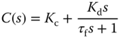
where  ,
,  and
and  are the proportional gain, the derivative control gain and the filter time constant, respectively.
For this type of controller design, we assume that the continuous time system is a second order with the transfer function:
It is not a straightforward task to choose the parameters  ,
,  and
and  based on the second order model (3.35). However, the PD controller can be converted into the classical lead-lag compensator that has the following form:
where the parameters  ,
,  are
are  are related to
  ,
,  and
and  via the relations below:


The lead-lag compensator in (3.36) can be designed by positioning the desired closed-loop poles on the left half of the complex plane.
With the lead-lag compensator, the actual closed-loop characteristic polynomial is a third order, which is

By choosing a third order desired closed-loop characteristic polynomial having the following form,

and letting  , we obtain the following linear equations:
The parameters are found via the solution of the linear equations as
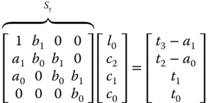
The polynomial equation  is called Diophantine equation, which is the essential step for finding the controller parameters in the pole assignment controller design. The matrix with the dimensions
  in (3.40) is called the Sylvester matrix, which is required to be invertible in the pole assignment controller design.
The following tutorial summarizes the computational procedure for finding the parameters for the PD controller with filter. We will use this program later on for applications.
For many applications, the second order model is simplified as

and the PD controller parameters have the following solutions:
3.3.2 Analytical Examples for Ideal PID with Pole-zero Cancellation
When designing a PID controller, the pole–zero cancellation technique is widely used in the application field. The main reason behind this practice is that with the pole–zero cancellation technique, the controller parameter calculations become very simple and can be performed using pencil on the back of an envelope. However, there are two important rules regarding the pole–zero cancellation technique. Firstly, an unstable pole or zero in the system should not be canceled because the cancellation will lead to an internally unstable system, for the reason that the canceled pole or zero is still part of desired closed-loop poles (see Section 2.5). Secondly, a stable pole close to the imaginary axis, which is a pole corresponding to a large time constant, in the system should not be canceled because the slow pole will re-appear to become the dominant pole in the closed-loop response to input disturbance, and as a result, slow disturbance rejection will occur (see the sensitivity analysis in Chapter 2). As a general rule, a stable pole or zero could be canceled if its position is on the left-hand side of the desired closed-loop poles on the complex plane. Additionally, it is the faster stable pole in the plant model that gets canceled.
We assume that there are two poles in a second order model and both are real, stable poles. With these assumptions, the transfer function is expressed as
where  is positive and
  .
.
The PID controller is assumed to have the ideal structure,
and an implementation filter will be added at the implementation stage with a small  parameter chosen by the designer (see Section 1.2). This means that the parameter
  will not be considered in the design stage. We will deploy a technique called pole–zero cancellation in the PID controller design, and with this technique the controller parameter solutions become very simple.
We re-write the PID controller given in (3.47) into the transfer function form,
By comparing (3.48) with (3.47), we have the relationships,
Thus, we find the parameters in (3.48) first, then convert them into the PID controller parameters required in the implementation stage.
When using the pole–zero cancellation technique, we assume that the numerator of the controller  is factored and the controller now has the form,
By choosing the zero of the controller  equal to the pole of the model
  (i.e.
(i.e.  ), we canceled the pole in the model with the zero in the controller. The net effect of this is that the relationship
  is simplified into
the closed-loop transfer function between the reference signal  and the output
  becomes
Note that the free parameters in (3.52) are  and
and  , respectively, and its denominator is a second order polynomial. The design becomes identical to the case when we designed the PI controller using pole assignment technique. Thus, by choosing the desired closed-loop characteristic polynomial as
with  and
and  or
or  , and equating the desired closed-loop characteristic polynomial with the denominator of (3.52), we obtain the polynomial equation,

By comparing both sides of (3.54), the free parameters are determined as
With the parameters, the PID controller is re-constructed with the information  as
as
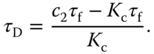
Its actual parameters are expressed using (3.49) as
3.3.3 Analytical Examples for PID Controllers with Filters
As the system becomes more complicated, a derivative filter needs to be used as part of the PID controller design to give an extra degree of freedom in the solution of the controller parameters. This is important in eliminating the approximation introduced by choosing a filter time constant in the implementation stage, hence enhancing the robustness of the PID control system.
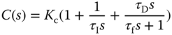
The general form of PID controller is defined by the transfer function
where  is a parameter that needs to be utilized as part of the derivative filter. However, the industrial control systems are often defined in terms of the PID controller parameters,
  ,
,  ,
,  , and a filter time constant
  . 1
. 1
Thus, we need to find PID controller parameters that lead to a completely identical configuration between the controller  defined by (3.62) and an industrial PID controller. With this in mind, we will choose the PID controller parameters such that
is identical to the PID controller in (3.62). The problem is solved using reverse engineering by expressing (3.63) as
which should be exactly equal to (3.62). By comparing these two expressions, we obtain,


We solve the PID controller parameters using these four linear equations and their values are,


The following example will examine the effect of pole–zero cancellation on reference following and disturbance rejection.
When the plant is underdamped, the pole–zero cancellation technique we used before will be avoided for the reason that the plant pole that was canceled in the design will re-appear in the closed-loop system for input disturbance rejection.
3.3.4 PID Controller Design without Pole–Zero Cancellation
We assume that the PID controller has the form,

and the second order model has the form,

Without pole–zero cancellation, the open-loop transfer function is
The closed-loop transfer function is

Note that the denominator of the closed-loop transfer function is a fourth order polynomial and there are four unknown controller parameters to be determined in the design. Thus, the desired closed-loop characteristic polynomial  must be a fourth order polynomial with all zeros on the left half of the complex plane. For instance, we can assume that
  has the form,

where the dominant poles are  (
( or 1), and
  . For simplicity, the desired closed-loop characteristic polynomial
  is denoted as
  . To assign the closed-loop poles to the desired locations, we solve the Diophantine equation,

By multiplication and collecting terms, we find the exact quantity on the left-hand side of (3.120), which is equal to its right-hand side:

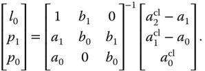
By comparing both sides of (3.121), a set of linear equations is formed,

This set of linear equations is expressed in matrix and vector form for convenience of solution,
where we assume that the square matrix  (called the Sylvester matrix) is invertible.
3.3.5 MATLAB Tutorial on Solution of a PID Controller with Filter
3.3.6 Food for Thought
- Would you design a PD or a PID controller for a first order system?
- If a system has a pole located on the right half of the complex plane (unstable pole), can you choose a controller zero to cancel this unstable pole?
- Is it correct to say that the open-loop pole that was cancelled in the design will re-appear at the output response to input disturbance?
- Is it correct to say that the open-loop pole that was cancelled will re-appear at the output response to output disturbance?
- Is it correct to say that the open-loop pole that was cancelled will re-appear at the output response to reference signal?
- How would you deal with time delay when using pole-assignment controller design technique?
- In the general pole-assignment controller design (without pole-zero cancellation), what is the condition required to obtain unique solutions of controller parameters?
3.4 Resonant Controller Design
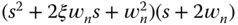
The resonant controller, different from the PI or PID controller, incorporates the factor  in the denominator of the controller. With the embedded mode, the closed-loop feedback control system is designed to be stable, and at the steady-state the output of the control system will completely track the sinusoidal signal and/or reject a sinusoidal disturbance signal that contains the frequency
  without any steady-state errors (see Section 2.5.3).
3.4.1 Resonant Controller Design
Consider a first order transfer function that is used to describe the dynamics of an AC motor with the form,
where the input is the torque current and the output is velocity. The task is to design a controller  to reject a sinusoidal disturbance with frequency
  (
( ). Pole-assignment controller design will be used here.
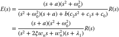
For the first order system, the controller structure is chosen as
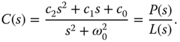
Here, the denominator of the controller is second order ( ), the numerator is also chosen to be second order to allow proportional control action. This choice leads to three unknown coefficients
  ,
,  , and
, and  to be determined. The actual closed-loop characteristic polynomial is

This is a third order polynomial. Therefore, the desired closed- loop characteristic polynomial should be third order and the number of desired closed-loop poles should be 3 accordingly. For instance, we can assume that the desired closed-loop characteristic polynomial  has the form (
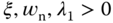 )
)

where the dominant poles are  (
( or 0.707), and
  . For simplicity, the desired closed-loop characteristic polynomial
  is denoted as
  .
.
With the pole assignment controller design technique, we let the actual closed-loop characteristic polynomial equal the desired closed-loop characteristic polynomial, which leads to,

This equation 3.137 is called the Diophantine equation. By substituting the expressions of  ,
,  ,
,  ,
,  , and
, and  into (3.137), the Diophantine equation is written as

In order for the left-hand side of the equation to be equal to the right-hand side of the equation, we have the following linear equations:
Solving these linear equations gives the coefficients of the controller as
3.4.2 Steady-state Error Analysis
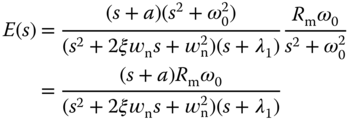
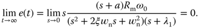
To show that the output of the closed-loop control system will follow a sinusoidal signal with frequency  , we calculate the closed-loop feedback error signal
  in relation to the sinusoidal reference signal
  . Here, the control signal is
and the output signal is
Noting that  , by substituting this into (3.146), we obtain
The relationship between the reference signal  and the output signal
  is
is
where we have used the Diophantine equation 3.137. When the reference signal  , its Laplace transform is
 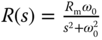 . From (3.148), we have the Laplace transform of the feedback error signal,
where we have canceled the factor  . Since the denominator of (3.149) contains all zeros on the left half of the complex plane, by applying final value theorem, we obtain
Because 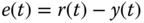 and
and 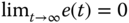 , we conclude that the output
  will converge to the reference signal
  .
.
To show that the closed-loop control system will completely reject a sinusoidal disturbance, we will find the relationship between the input disturbance and the output. Here, the transfer function between the input disturbance  and the output
  is
is
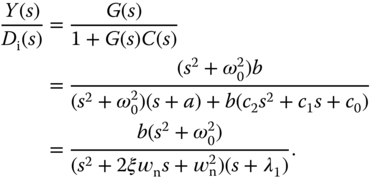
Assume that the disturbance signal is a sinusoidal signal 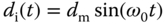 with unknown amplitude
  , and it has the Laplace transform
 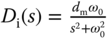 . Thus, the output in response to the input disturbance
  is
is
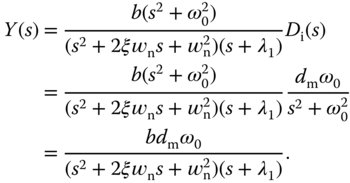
The zeros of the denominator are all on the left half of the complex plane as the parameters  ,
,  , or 1 and
  . Thus, by applying final value theorem, we obtain
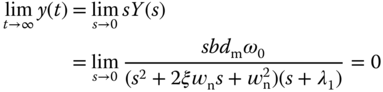
Therefore, the output  in response to the input disturbance
  is zero at the steady-state. This means that the input disturbance
  will be completely rejected by the closed- loop feedback control system.
3.4.3 Pole–Zero Cancellation in the Design of a Resonant Controller
With the resonant controller, as shown in Section 2.5.3, the complementary sensitivity function is required to satisfy  at the frequency
  . Thus, this indicates that the bandwidth of the closed-loop resonant control system is to be greater than
  , at least. If
  is large, from the analysis given in Chapter 2, this implies in general that a resonant control system requires a better mathematical model for robustness and better sensors for noise attenuation.
3.4.4 Food for Thought
- A periodic reference signal has a known frequency 50 Hz. What is the frequency parameter
 you would use in the design of resonant controller so that the reference signal could be tracked without steady-state error?
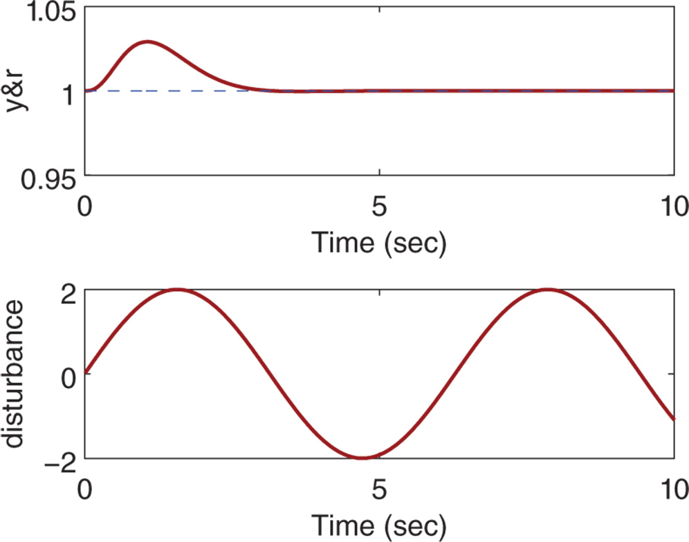
Figure 3.10 Sinusoidal input disturbance rejection (Example 3.10).
- If a resonant controller is designed to track a sinusoidal signal with frequency
 without steady-state error, will the same resonant controller reject a periodic input disturbance signal with the same frequency?
 - If the sinusoidal reference signal is known to have the frequency
 and the disturbance is known to have a frequency
  , is it correct to choose the denominator of the resonant controller to contain the factor
 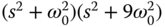 ?
? - If the reference signal is a sinusoidal signal with frequency
 plus a constant, what would be the key factors in the denominator of the resonant controller you would choose so that the closed-loop control system will track this reference signal?
3.5 Feedforward Control
Feed forward control is widely used in combination with either PID or resonant controllers. The starting point for feedforward compensation is that the feedforward variables used are either directly measured or estimated. Their effect is captured at the control signal from which it can be subtracted. It has various forms; however, the basic idea remains the same.
3.5.1 Basic Ideas about Feedforward Control
Assume that the output of a dynamic system is described by the Laplace transform:

where  is the Laplace transform of the control signal and
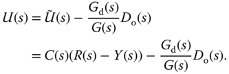
  is the disturbance that is measured and used in the feedforward compensation. To introduce feedforward compensation, (3.175) is re-written as
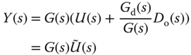
where an intermediate control signal  is defined as
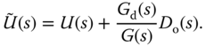
Based on (3.176), a PID controller  is designed using the transfer function
  to generate the intermediate control signal
  from which the effect of the disturbance
  is subtracted. This explicitly leads to the actual control signal
  to be expressed as
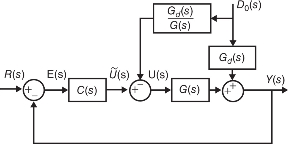
Figure 3.11 Block diagram of the feedback and feedforward control system.
Clearly, the assumption is that the transfer function  is stable and realizable in addition to
  being measured. Figure 3.11 illustrates the feedback and feedforward control system. As an example, if we assume that
  and
and  are represented by the following first order plus delay transfer functions:
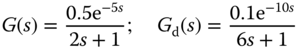
then the control signal  is expressed as
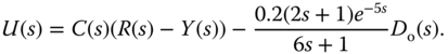
Because the time delay of the disturbance model is larger than the time delay of the plant model, the transfer function  is realizable, hence the feedforward compensation can be implemented for the application.
3.5.2 Three Springs and Double Mass System
To illustrate how to use a feedforward controller in conjunction with a PID controller, we will examine the PID control system design for a three springs and double mass system.
A three springs and double mass system Tongue (2002) is illustrated in Figure 3.12. In this figure, the two blocks are with mass  and
and  , and there are two spring constants
  for the right and left springs,
  for the middle spring. The manipulated variables are the two applied forces
  and
and  and the output variables are the distances of the mass block movement
  corresponding to block one and
  corresponding to block two.
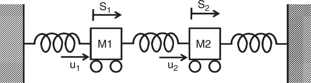
Figure 3.12 Three springs and double mass system.
We consider the simplified spring force  where
where  and
and  is the distance of the mass movement, and apply Newton's law 2 to the first block to obtain the following equation:
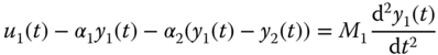
where the first term represents the first external force, the second and third terms represent the forces from spring 1 and spring 2, respectively. The right-hand side of (3.178) is the multiplication of the mass and acceleration of block 1. Similarly, by applying Newton's law to the second block, we obtain
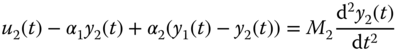
where the first term represents the second external force, and the second and the third terms are the forces generated from spring 3 and spring 2. The right-hand side of (3.179) is the multiplication of mass and acceleration of block 2.
To have a clear view of the dynamics, we re-write (3.178) and (3.179) as
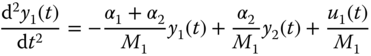
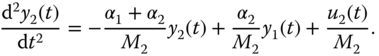
We have two second order systems for the three springs and double mass system. Additionally, there are interactions between the two systems.
As in Tongue (2002), the physical parameters are  kg,
kg,  kg,
kg,  N
N  and
and  N
N  . As an exercise, the parameter is varied to
  N
N  .
.
3.6.2.1 PID Controller with Filter
The PID controller with filter is designed based on the transfer function model (3.182) using the MATLAB program PIDplace.m (see Tutorial 3.2). The term  is considered as disturbance. Two pairs of complex poles are used in the pole assignment PID controller design. With damping coefficient
  , the parameter
  is used as a performance tuning parameter. Because of the interactions between the two outputs, the closed-loop dynamics from the first mass block are more complex. As a result, there is a minimum
  required for the stabilization of the closed-loop system. Through simulation studies, this minimum
  is approximately five times the natural frequency of the original system. This behavior is similar to that of controlling unstable systems where a minimum controller gain is required for robustness of the feedback system.
By selecting  and
and  for the two pairs of complex poles, the program PIDplace.m calculates the PID controller parameters as

Closed-loop Simulation Studies
In the first simulation, we assume  for
for  . However, because the second mass is connected to the first mass, the output
  is not zero. With sampling interval
  (s), a step reference signal with amplitude 0.1 is added to the closed-loop control. Figure 3.13(a) shows the control signal used to move the first mass from the origin to 0.1 m and Figure 3.13(b) shows the output signal. It is clearly seen from Figure 3.13(a) that the second mass generates a sinusoidal disturbance and the feedback control signal tries to compensate it. The effect of the sinusoidal disturbance is hardly noticeable. Another simulation scenario is presented. Assume that there is a constant negative force acting on the second mass block, which is
  . Additionally, the control signal
  is constrained to positive values (
 ). Figure 3.14 shows the closed-loop responses for the three springs and double mass system with
  . The control signal (see Figure 3.14(a)) still tries to reduce the effect of the disturbance, however because of its larger amplitude, the effect of the disturbance can be seen from the output response (see Figure 3.14(b)).
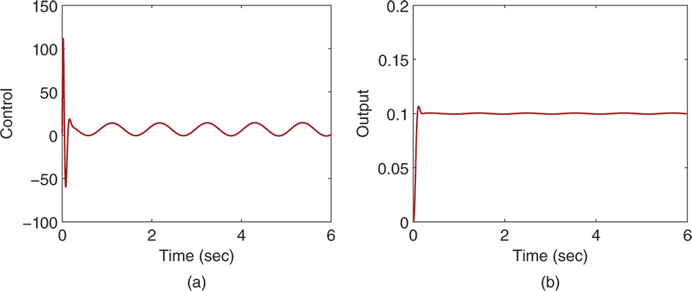
Figure 3.13 Closed-loop responses for three springs and double mass system with  (Example 3.11). (a) Control signal. (b) Output signal.
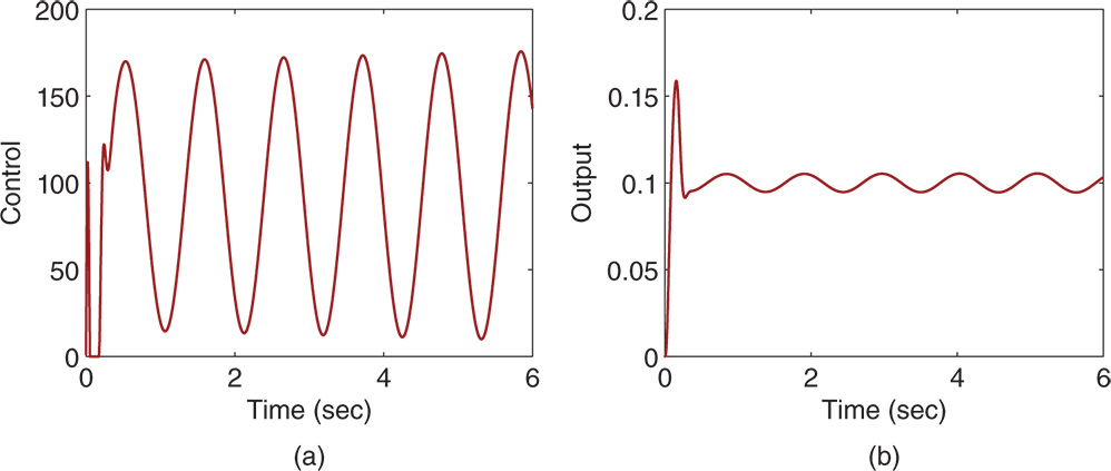
Figure 3.14 Closed-loop responses for three springs and double mass system with  (Example 3.11). (a) Control signal. (b) Output signal.
3.5.3 Food for Thought
- In the feedforward control, if the feedforward variable is bounded, as shown in the three springs and double mass system, would you believe that the feedforward control will not cause closed-loop instability?
- In most of the applications when using feedforward compensation, the feedforward variable is captured as part of the control signal as shown in the three springs and double mass system so it is conveniently subtracted. Can we extend this idea of feedforward compensation to the reference signal?
- What are the main advantages of using feedforward control?
- What are the drawbacks of using feedforward control?
3.6 Summary
This chapter has discussed one of the most widely used control system design methods for PID and resonant controllers. The central ideas behind the pole-assignment controller design are to specify the desired closed-loop performance via the locations of the closed-loop poles and to match the desired closed-loop poles with the actual closed-loop poles by finding the solutions of a polynomial equation. These methods are conceptually and computationally simple, and the design methodology can be extended to various controller structures and models. The other important aspects are summarized as follows.
- For a first order model, we can design a P controller or a PI controller or a resonant controller.
- For a second order model, we can design a PD controller or a PID controller or a resonant controller with a first order filter.
- For a higher order model, the structure of the controller needs to be selected so that the controller parameters can be determined uniquely.
- We can use the pole-zero cancellation technique for the purpose of getting simple analytical solutions. We can only cancel the poles corresponding to fast dynamic response. The canceled poles will re-appear in the closed-loop system in response to input disturbance. We can not cancel unstable poles or zeros in the design.
- For a higher order system, model order reduction is used to obtain first order or second order model for the PID controller design.
- The locations of the desired closed-loop poles are chosen, and they need to be adjusted to suit the requirement of closed-loop response speed for reference following, disturbance rejection, noise attenuation and robustness of the closed-loop system. It will be desirable to adjust them according to the Nyquist diagram and the sensitivity analysis presented in Chapter 2.
3.7 Further Reading
- Internal model control is introduced in the book Morari and Zafiriou (1989).
- Pole-assignment PID controller design together with several other design methods are introduced in Goodwin et al. (2000),Cominos and Munro (2002).
- Robust pole-assignment controller design is proposed in Soh et al. (1987), Nurges (2006), Wang et al. (2009).
- Pole-assignment in combination with sensitivity shaping is proposed in Langer and Landau (1999).
- Self-tuning control using pole-assignment design is one of the original self-tuning controllers Wellstead et al. (1979).
- Pole-assignment PID controller design with dominant pole consideration and analysis is introduced in Zítek et al. (2013).
- With approximation of time-delay and specification of a desired closed-loop time constant, PI and PID controllers are found analytically using direct synthesis method for disturbance rejection (Chen and Seborg (2002)).
- A simple relay nonlinear PD controller is proposed for controlling high precision motion system with frictions (Zheng et al. (2018)).
- Current control in electrical AC drives and power converters typically uses PI control structures in the synchronous reference frame (
 reference frame) because their reference signals are constant (Wang et al. (2015)). If the stationary reference frame is used, then current control for the AC drives and power converters utilizes resonant controllers because their reference signals are sinusoidal (Wang et al. (2015)).
Problems
- 3.1 Design PI controllers for the systems with the transfer function
 , where the parameters
  and
and  are given as follows:
 and
and  ;
; and
and  ;
; and
and  .
.
In the design, the desired closed-loop characteristic polynomial is selected as
 with
with  and choosing the natural frequency parameter
  as
as  ,
,  and
and  . Compare the proportional controller gain
  and the integral time constant
  for the three choices of the bandwidth. What are your observations?
 - 3.2 PD controllers are designed based on a second order model, which has the following form:

- Find the PD controllers with a derivative filter for the following systems:
 ,
,  ,
,  ,
,  .
. ,
,  ,
,  ,
,  .
. ,
,  ,
,  ,
,  .
.
where all the desired closed-loop desired closed-loop polynomial is chosen to be
 , where
  and
and  .
. - Write a Simulink simulation program to evaluate the performance of the three closed-loop PD control systems with a unit step reference signal using sampling interval
 (sec), where the derivative control is implemented on the output only. Will the closed-loop output follow the reference signal without steady-state error?
- Find the PD controllers with a derivative filter for the following systems:
- 3.3 In the design of a PI controller, it is often to approximate a higher order system with a first order transfer function where the dominant time constant is identified (largest time constant) and kept, while the other smaller time constants are neglected. This follows the procedure of writing the transfer function using the form
where we assume that
 .
.- Design PI controllers for the following systems with appropriate approximation of the complex dynamics. The desired closed-loop performance is specified using the polynomial
 , where
  and
and  is
is  .
.
 ;
; ;
; . (Hint: use Pade approximation to the time-delay in order to find the dominant dynamics,
  )
)
- Evaluate the closed-loop stability by using Nyquist diagram. If the closed-loop system is unstable, reduce the parameter
 to achieve stable closed-loop system.
 - Simulate the closed-loop step response for the PI controlled systems with sampling interval
 .
. - If the closed-loop response were oscillatory, reduce the parameter
 until satisfactory performance is achieved.
- Design PI controllers for the following systems with appropriate approximation of the complex dynamics. The desired closed-loop performance is specified using the polynomial
- 3.4 Find the PID controller parameters using pole-assignment controller design technique and apply pole-zero cancellation to simplify the parameter solutions. Here, the PID controller structure is assumed to be
 . Take approximation of the complex dynamics if necessary. The desired closed-loop characteristic polynomial is
  where
where  and
and  is adjusted for each case. The transfer functions with performance specification are given as below:
 , and
, and 
 , and
, and  .
. , and
, and  .
. , and
, and  .
.
- 3.5 Find the parameters for PID controller with a filter using pole-assignment controller design technique. Use pole-zero cancellation technique to simplify the parameter solution and take approximation of the complex dynamics if necessary. With a pole-zero cancellation, the desired closed-loop polynomial is specified as
 . The transfer functions with performance specification are given as below:
 ,
,  and
and  .
. ,
,  and
and  .
.
- 3.6 For a system with the transfer function
design a controller with the structure
where all three desired closed-loop poles are chosen to be
 . Convert this controller into an ideal PID controller that has the structure
  so to find the proportional gain
  , integral time constant
  and the derivative time
  . Use final value theorem to show that for a step reference signal with amplitude
  , the closed-loop output response is
  as
as  . The following three systems are used in this exercise.
 ,
,  ,
,  .
. ,
,  ,
,  .
. ,
,  ,
,  .
.
- 3.7 For a system with the transfer function

design a resonant controller with the structure
where all three desired closed-loop poles are chosen to be
 . Supposing that the reference signal is a sinusoidal signal
  , show that as
  , the feedback error
  . The following three systems are used in this exercise.
 ,
,  , and
, and  .
. ,
,  , and
, and  .
. ,
,  , and
, and  .
.
- 3.8 In order for the closed-loop system to track a reference signal
 , the controller needs to contain the factors
  and
and  in its denominator. For a system with the transfer function

design a resonant controller plus integral action with the structure

where all four desired closed-loop poles are chosen to be
 . Supposing that the reference signal is a sinusoidal signal
  , show that as
  , the feedback error
  . The following three systems are used in this exercise.
 ,
,  , and
, and  .
. ,
,  , and
, and  .
. ,
,  , and
, and 
- 3.9 A robot arm is described by the second order transfer function:
(3.187)

where the input is the voltage and the output is the position of the arm on x-axis.
- Design a resonant control system such that the output of the robot arm will follow a sinusoidal reference signal
 without steady-state error. All desired closed-loop poles are positioned at
  (hint: use pole-zero cancellation technique to simplify the computation).
 - Verify your design by showing that the error signal (
 ) converges to zero as time
  . That is

Write a Simulink simulation program to evaluate the closed-loop system performance for reference following of the sinusoidal signal where the sampling interval
 .
. - Now, suppose that the reference signal contains a constant 10, leading to the new reference signal
 . Show that with this resonant controller, the error signal (
 ) also converges to zero as time
  . Modify the Simulink simulation program to include the new reference signal and confirm that the closed-loop output tracks the new reference signal without steady-state error.
 - Assume that the input disturbance
 enters the system at half of the simulation time, where
  and
and  . Modify the Simulink simulation program to include the disturbance and confirm that the resonant controller can not completely reject this input disturbance. What would you propose for the resonant controller structure so that it will reject this disturbance without steady-state error? Verify your answer using final value theorem.
- Design a resonant control system such that the output of the robot arm will follow a sinusoidal reference signal
- 3.10 An unstable system is described by the transfer function:
(3.188)
where
 and
and  .
.- Design a PI controller to control this system, where all desired closed-loop poles are positioned at
 .
. - In order to guarantee the closed-loop stability of the PI control system, the magnitude of the stable pole
 has a relationship with the unstable pole
  . Use Routh-Hurwitz stability criterion to find this relationship.
- Design a PI controller to control this system, where all desired closed-loop poles are positioned at
 was previously linked to the derivative gain
  as
as  .
. , where
  is the total force,
  is the mass and
  is the acceleration.