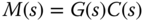
2
Closed-loop Performance and Stability

2.1 Introduction

Because feedback control can cause a closed-loop system to become unstable, ensuring closed-loop stability is paramount in control system design. In Section 2.2, we will discuss closed-loop stability by examining the locations of closed-loop poles and the applications of the Routh–Hurwitz stability criterion. In Section 2.3, the Nyquist stability criterion is presented based on a frequency response analysis, which leads to conclusions of closed-loop stability by examining the frequency response of the loop transfer functions, particularly convenient for analysis of systems with time delay.

To understand the roles of external signals playing in a feedback control system, Section 2.4 introduces control system structures with different degrees of freedom, which are related to the topic of reducing overshoot in reference response discussed in Chapter 1. Also in this section, the sensitivity functions are introduced in relation to various external signals in the closed-loop system. In Sections 2.5 and 2.6, we will examine the key issues existed in a feedback control system that are related to reference following, disturbance rejection, and noise attenuation from the angles of sensitivity analysis. The final section of this chapter will discuss the robust stability using frequency response analysis. Many examples presented in this chapter use PID controllers designed with the tuning rules given in Chapter 1.

2.2 Routh–Hurwitz Stability Criterion

Feedback control can cause a system to become unstable. Ensuring closed-loop stability is the most important aspect in control system design. Therefore, for every control system designed, its closed-loop stability is required to be checked as the top priority.

For linear time invariant systems, there are two main categories of methods that have been widely used to check closed-loop stability. The first type is based on the direct computation of the poles of the closed-loop transfer function. We call them the closed-loop poles. If all the closed-loop poles have negative real parts, namely with all poles strictly on the left half of the complex plane, then the closed-loop system is stable. If there are one or more poles on the right half of the complex plane, having a positive real component, then the closed-loop system is unstable. If there are one or more poles with real part equal to zero, namely on the imaginary axis of the complex plane, we call this type of system marginally stable. The second type is based on the open-loop transfer function that includes the plant transfer function, sensor and actuator transfer functions, and the controller transfer function. The Nyquist stability criterion is one of the most widely used methods that is based on the open-loop frequency response analysis.

2.2.1 Determining Closed-loop Poles

The first step in the computation of closed-loop poles is to calculate the closed-loop transfer function. Once the closed-loop transfer function is determined, then the MATLAB function roots.m is used to find the zeros of the denominator of the closed-loop transfer function, which are the poles of the closed-loop transfer function.

Note that in the computation of the closed-loop transfer function, the sensor and actuator dynamics will be considered in addition to the controller transfer function.

---

Example 2.1

Consider the process described by the transfer function:

(2.1)

where we assume that both sensor and actuator dynamics are included in the transfer function. Use IMC-PI controller tuning rules to determine the PI controller parameters and find the closed-loop poles.

Solution From Skogestad (2003), the second order system (2.1) is approximated by the first order plus delay model:

According to the IMC-PID controller tuning rules, the proportional gain and the integral time constant are calculated as

where the closed-loop time constant is selected as .

Now, to calculate the closed-loop poles, we write the original the transfer function as

and the controller transfer function as

(2.2)

(2.3)

Note that in the calculation of the closed-loop poles, we need to use the original process model (2.1), not the first order plus time delay model. The closed-loop block diagram is illustrated in Figure 2.1.

Figure 2.1 Closed-loop control system in transfer function form.

The closed-loop transfer function from the reference signal to the output is calculated as

(2.4)

Clearly, the denominator of the closed-loop system is and the closed-loop poles are the solutions of the polynomial equation:

(2.5)

This polynomial equation is called the closed-loop characteristic equation. For this example, we have

We use the MATLAB roots.m function as

den=[0.2000  1.2000  1.9167  0.8333];
roots(den) 

and find the three closed-loop poles as Clearly, the closed-loop IMC-PI control system is stable with all poles on the left half of the complex plane. The closed-loop system has three closed-loop time constants. The dominant time constant is the largest calculated using the smallest magnitude of the closed-loop pole as

We pay attention to the largest time constant because it determines how fast the closed-loop response will be. For instance, this time constant is larger than the dominant process time constant, which is equal to 1. We may conclude that the closed-loop system response speed is slower than the open-loop process response speed because the closed-loop dominant time constant is larger.

---

2.2.2 Routh–Hurwitz Stability Criterion

It would not be a straightforward task if we had to calculate the closed-loop poles using pencil and paper for a third order system and above. The Routh–Hurwitz stability criterion was introduced in the development of control systems early on so that their closed-loop stability could be determined using pencil and paper. Without involving complex computation, using the Routh–Hurwitz stability criterion enables us to determine whether there are any closed-loop poles on the right half of the complex plane and how many of them there are. This simple calculation is performed using the coefficients of the denominator of the closed-loop transfer function.

Table 2.1 Routh–Hurwitz table.

				…
				…
sn−2	r2,1	r2,2	r2,3	…
sn−3	r3,1	r3,2	r3,3	…
⋮	⋮
s2	rn−2,1	rn−2,2
s	rn−1,1
s0	rn,1

In general, for the denominator of the closed-loop transfer function with the polynomial

we use its coefficients to form the first two rows of the Routh–Hurwitz table (see Table 2.1), and based on the first two rows complete the rest of the elements in the table. The first element in the third row is

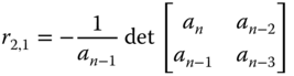
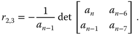
where it is seen that we used the nearest two previous rows to form the determinant scaled by the factor . The second element in the third row is

which is the same scaling but with the replacement of the next column in the determinant. With the same pattern,

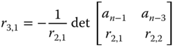
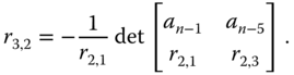
For the fourth row, we will use the elements in the nearest two rows (second and third rows) with the same pattern, where

The remainder of the elements are expressed in a general form as

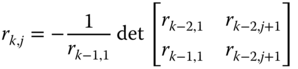
where .

The elements in the first column of the Routh–Hurwitz table will determine whether the closed-loop system is stable. The number of roots of the polynomial with real part greater than zero is equal to the number of sign changes in the first column of the Routh–Hurwitz table. Simply, if the first coefficient in is positive, then closed-loop stability will follow if all elements in the first column are positive.

Note that, in the calculation of the table, if an element in the first column becomes zero, then the calculation continues by replacing the zero element with a variable . The remainder of the elements will be expressed in the function of . Closed-loop stability will be determined by examining the coefficients in the first row using .

If the coefficients of the closed-loop transfer function are constant and known, the closed-loop poles are simply calculated using the MATLAB function roots.m, as illustrated in Example 2.1. However, the Routh–Hurwitz stability criterion is very effective in determining closed-loop stability when some of the controller or process parameters have uncertainties.

---

Example 2.2

Continuing from Example 2.1, determine the minimum value of in the IMC-PID tuning rule to produce a stable closed-loop system.

Solution From the controller transfer function (2.3), we can express the variation in the controller parameters as

where . Therefore, the closed-loop polynomial becomes

From the closed-loop polynomial, we obtain the first two rows in the Routh–Hurwitz table (see Table 2.2).

The parameter is calculated using the following formulae:

To ensure closed-loop stability, we require , which means that

Therefore . The parameter is calculated as

Table 2.2 Routh–Hurwitz table for the third order system.

	0.2	1.9167
	1.2
s1	x1	0
s0	x2	0

The requirement of means that .

Combining the imposed conditions from and , we conclude that closed-loop stability is ensured if . One can verify using the MATLAB roots.m function that when , the three closed-loop poles are: . The closed-loop system is marginally stable because a pair of its poles is on the imaginary axis of the complex plane. For any less than 0.07971, the closed-loop system becomes unstable.

This example also indicates that there is a limit on what value we can select for the parameter in the IMC-PID controller tuning rules.

---

2.2.3 Food for Thought

1. For a given system, when the closed-loop poles are found to be , and , what kind of behavior do you expect the closed-loop output response to be?
2. When the closed-loop poles are found to be , what kind of output response do you expect?
3. Why do the complex poles always appear in a complex conjugate form?
4. Can we determine closed-loop stability if one of the coefficients in the leading column of Routh-Hurwitz stability criterion is zero?
5. Can we apply Routh-Hurwitz stability criterion to systems with time delay?

2.3 Nyquist Stability Criterion

The Nyquist stability criterion is one of the most widely used tools in analyzing closed-loop stability. Using MATLAB graphic tools, the Nyquist diagram is very easy to produce by calculating the frequency response of the loop transfer function. The gain margin, phase margin and delay margin provide valuable insight into closed-loop stability with respect to parameter variations.

2.3.1 Nyquist Diagram

The Nyquist stability criterion uses the frequency response of an open-loop system, including the plant, the sensors and the actuator, to determine closed-loop stability. Here, the open-loop system is expressed as

where represents the system dynamics including the plant dynamics, the actuator dynamics, and the sensor dynamics, and represents the controller transfer function. More specifically, it is a graphic approach using real and imaginary values of the frequency response where is that of the loop transfer function. The benefit of being a graphic approach lies in the intuition as well as both quantitative and qualitative measures.

As an illustration, the Nyquist loci of a PI controlled system that has a stable open-loop transfer function with time delay is shown in Figure 2.2, where the following loop transfer function is used:

(2.6)

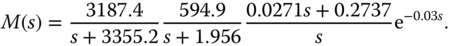
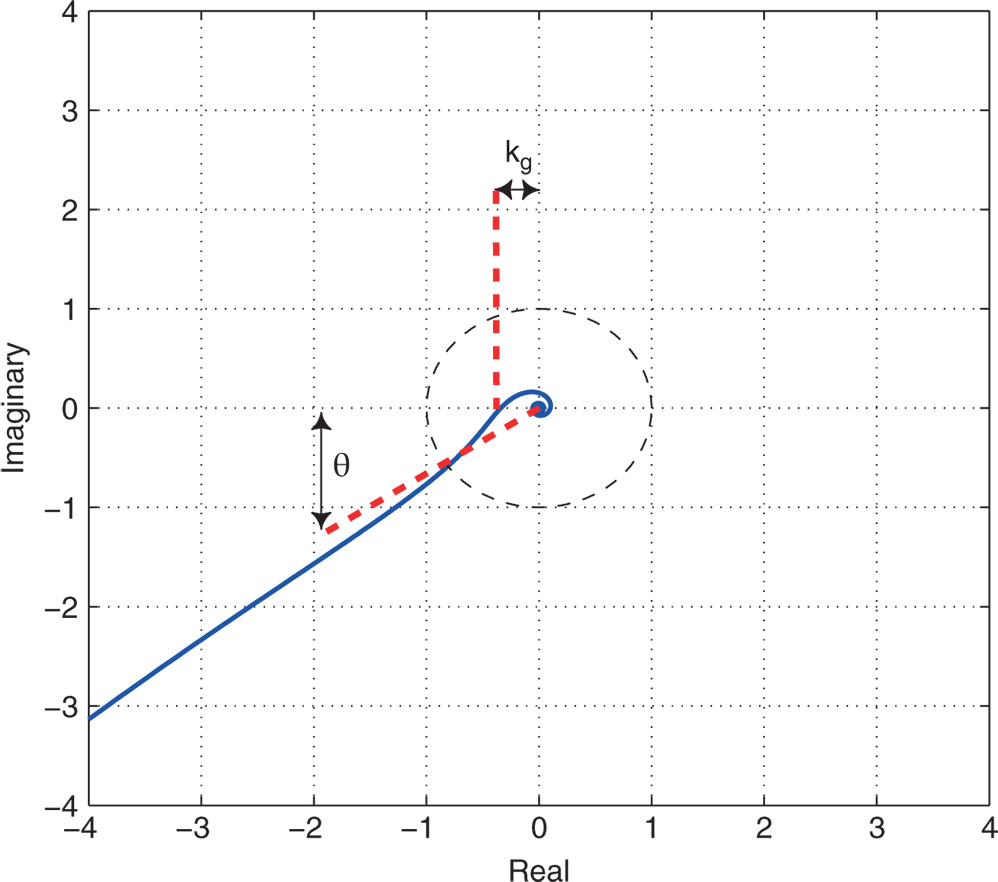
Figure 2.2 Nyquist plot with a unit circle for illustration of gain margin and phase margin. Solid line: Nyquist loci; dashed lines: pointers for the gain margin and phase margin.

We can specify the frequency vector and use the MATLAB function freqs.m to calculate the frequency response of the open-loop transfer function. The time delay component is computed first using the MATLAB exponential function and multiplied by the frequency response of the rest of the open-loop transfer functions. Tutorial 2.1 shows the MATLAB program for the Nyquist plot.

The Nyquist criterion states that a feedback control system with single input and single output is stable if and only if, for the frequency response of the loop transfer function , number of counter clockwise encirclements of the point is equal to the number of poles of this loop transfer function with positive real parts. Note that this criterion presents both necessary and sufficient conditions for closed-loop stability using its open-loop transfer function. There are two comments related as below.

1. For the majority of PID controlled systems, this loop transfer function does not contain any poles that have positive real parts. Thus, for closed-loop stability of these classes of systems, the Nyquist stability criterion simply becomes that the frequency response should not encircle the point on the complex plane.
2. Because it uses the frequency response, closed-loop stability for systems with time delay will be examined without approximation. This is one of the most important advantages for using Nyquist loci to analyze control systems.

There are several quantitative, yet intuitive measurements that can be derived from the Nyquist loci. These quantities, termed gain margin, phase margin, and delay margin, are frequently used to assess the performance of the designed control system using the frequency information and safe-guard the closed-loop system against future model uncertainties.

2.3.1.1 Gain Margin

Gain margin is a quantity that is used to measure how much variation in gain the feedback control system could sustain before it became unstable. As illustrated in Figure 2.2, the gain margin is defined as , where is the distance between the origin of the complex plane and the point that intersects the real axis (see the vertical dashed line in Figure 2.2). This means that if the loop gain were to exceed , then the closed-loop system would become unstable. The parameter can be easily determined from the Nyquist loci. Using the following MATLAB command:

[x,y]=ginput(1) 

a cross hair appears on the Nyquist plot. By overlaying the center of the cross hair on the point that the Nyquist curve intersects the real axis, we obtain the coordinates as and . The distance is . Therefore, the gain margin is determined as . This means that if we were to increase the loop gain to three times the original value, then the closed-loop system would become unstable. We can associate this gain margin with the variations in the steady-state gain of the plant, the sensor, the actuator, or the controller gain . It is the net effect of all the combined variations of gains.

2.3.1.2 Phase Margin

To identify the phase margin, we first draw a unit circle with its origin located at the origin of the complex plane, as shown in Figure 2.2, and a straight dashed line that connects the point when the circle intersects the Nyquist loci with the origin of the complex plane. The phase margin is the angle between the negative real axis and the dashed line. Clearly, it is the additional phase lag that could be associated with before the closed-loop system became unstable. The phase margin can be calculated using the following MATLAB function ginput.m. When using the following MATLAB function:

[x,y]=ginput(1) 

a cross hair appears. Overlaying the center of the cross hair on the point that the unit circle intersects the Nyquist loci, we obtain the coordinates of and for that point. From Figure 2.2, the coordinates are and . Then the phase margin is computed as

2.3.1.3 Delay Margin

Although the phase margin represents how much additional phase lag can be added to the feedback control system before it becomes unstable, it does not directly convey the size of maximum time delay that can be added to the system. To determine the maximum time delay that can be tolerated, we let

where is the delay margin or the maximum delay to be tolerated and is the frequency when the unit circle intersects with the Nyquist loci. This yields

Clearly, a larger would lead to a smaller delay margin given the same phase margin . Thus, the frequency is an important parameter. To determine the frequency , we will plot , as shown in Figure 2.3. Using the function ginput.m, we identify the intersecting point of the dashed line with the solid line in Figure 2.3 that has the coordinates and . Thus, . From the parameter and the phase margin , we calculate the delay margin as

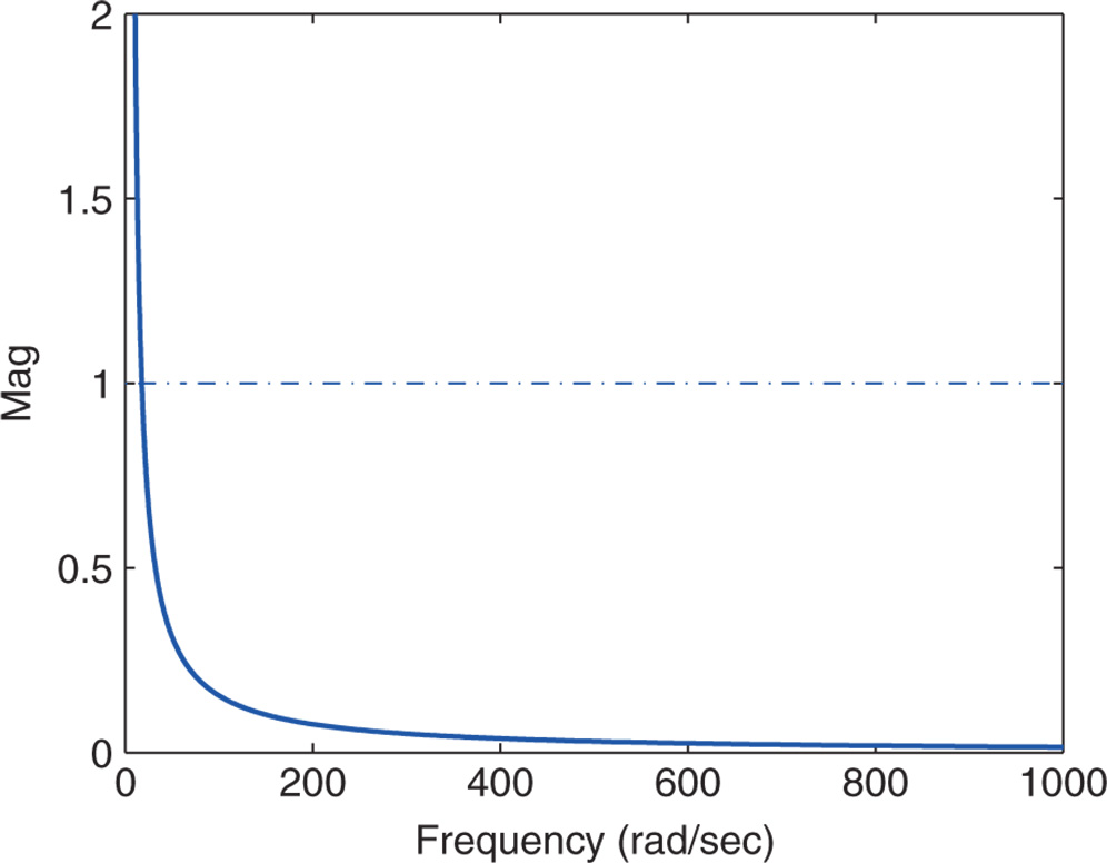
Figure 2.3 Magnitude of (solid line) together with dashed line to determine .

This means that the associated delay, which can be added to the system before it becomes unstable, is 0.0314 s.

---

Tutorial 2.1

This tutorial is to illustrate how to produce a Nyquist diagram using MATLAB functions. The open-loop transfer function used in the illustration is given by (2.6).

Step by Step

1. Create a new file called NyquistPlot.m.
2. We produce the transfer function using the three first order transfer functions with time delay. Enter the following program into the file:

   num1=3187.4;
   den1=[1 3355.2];
   num2=594.9;
   den2=[1 1.956];
   num3=[0.0271 0.2737];
   den3=[1 0];
   delay=0.03; 

3. Define the frequency vector and calculate the frequency responses of the three first order systems. Enter the following program into the file:

   w=logspace(-1,3,1000);
   G1=freqs(num1,den1,w);
   G2=freqs(num2,den2,w);
   G3=freqs(num3,den3,w);
   G12=G1.*G2;
   G123=G12.*G3; 

4. Add the component of time delay to the frequency response. Enter the following program into the file:

   j=sqrt(-1);
   Ny=G123.*exp(-j*w*delay); 

5. Present the two dimensional diagram with a unit circle that is centered at the origin of the complex plane. Enter the following program into the file:

   plot(real(Ny),imag(Ny),'b','linewidth',2)
   hold on
   th=[0:2*pi/60:(60)*2*pi/60];
   R=exp(j*th);
   plot(R)
   axis([-4 4 -4 4])
   xlabel('Real')
   ylabel('Imag') 

---

2.3.2 Rework of Tuning Rules based PID Controllers

---

Example 2.3

We examine the PI controllers presented in Example 1.7, where the continuous time plant has the transfer function:

(2.7)

Three sets of PI controller parameters were obtained by using the tuning rules of Ziegler–Nichols, Cohen–Coon and Wang–Cluett, as shown in Table 1.8. In this example, we analyze closed-loop stability for the three systems using Nyquist stability criterion, and modify the controller parameters to achieve closed-loop stability.

Solution. With the PI controller parameters listed in Table 1.8, the loop frequency response is computed and the Nyquist diagrams for the three PI controlled system are compared in Figure 2.4. It is seen from their Nyquist diagrams that the first two tuning rules produced the Nyquist loci encircling the point on the complex plane, hence they will lead to unstable closed-loop systems, which was confirmed by the Simulink simulation in Example 1.7. However, the Nyquist loci from the third tuning rule did not encircle the point, hence it produced a stable closed-loop system, which was also confirmed through simulation in Example 1.7. Using the MATLAB ginput function with the cross hair we can identify the gain margin for the third Nyquist loci as

and the phase margin as

The information derived from the Nyquist diagrams not only determines whether the closed-loop system is stable or not, but also provides us with an intuitive means to modify the controller parameters in order to achieve closed-loop stability. If we take 50% of the proportional controller gains from the first two tuning rules (i.e. and respectively), then all three PI controllers will produce a stable closed-loop system because all Nyquist plots will no longer encircle the point on the complex plane (see Figure 2.5). Table 2.3 summarizes the PI controller parameters and the associated gain margin, phase margin, and delay margin for this example, where Figure 2.6 is used to determine the delay margin.

Figure 2.4 Nyquist plots with a unit circle (Example 2.3). Key: line (1) using Ziegler–Nichols tuning rules; line (2) Cohen–Coon tuning rules; and line (3) using Wang–Cluett tuning rules.

Finally, the unit closed-loop step responses for the three PI control systems are computed using (s). Figure 2.7 compares the three closed-loop step responses. In this set of closed-loop simulation studies, the proportional control is implemented on the output only.

Figure 2.5 Nyquist plots for the modified controller with a unit circle (Example 2.3). Key: line (1) using Ziegler–Nichols tuning rules; line (2) Cohen–Coon tuning rules; and line (3) using Wang–Cluett tuning rules.

Table 2.3 Modified PI controller parameters with gain margin, phase margin, and delay margin.

			Gain margin	Phase margin	Delay margin
Ziegler–Nichols	3.2	108	1.4914	0.5305
Cohen–Coon	3.26	75.9231	1.258	0.2879	11.9461
Wang–Cluett	3.8867		1.2191	0.3184	12.585

Figure 2.6 Magnitude of (solid line) together with dashed line to determine . Key: line (1) using Ziegler–Nichols tuning rules with reduced ; line (2) Cohen–Coon tuning rules with reduced ; and line (3) using Wang–Cluett tuning rules.

Figure 2.7 Comparison of closed-loop step responses (Example 2.3). Key: line (1) Ziegler–Nichols tuning rules with reduced ; line (2) Cohen–Coon tuning rules with reduced ; and line (3) using Wang–Cluett tuning rules.

Overall, with the Nyquist diagrams and the closed-loop step response evaluations, the Ziegler–Nichols tuning rules with the reduced produced a slightly better control system. However, the Wang–Cluett tuning rules were applied as they were derived and not modified.

---

2.3.3 Food for Thought

1. What would happen to a closed-loop system if its gain margin is equal to 1?
2. Would you say that the Nyquist diagram is an effective means to check the performance of the PID controller designed when using the tuning rules?
3. What would you do if the gain margin of the control system designed is too small?
4. How would you be able to increase the phase margin of a control system?

2.4 Control System Structures and Sensitivity Functions

This section introduces control system structures with one and two degrees of freedom, which are related to the PID controller realization to reduce the overshoot in reference response discussed in Chapter 1. The external signals such as reference signal, disturbance signals and measurement noise are important in the analysis of control system performance. This section discusses these signals in relationships with the sensitivity functions.

2.4.1 One Degree of Freedom Control System Structure

A feedback control system of a one degree of freedom structure is represented by the block diagram, shown in Figure 2.8, where is the reference signal, is the output, and is the control signal. There is also an output disturbance in the system, denoted as . For simplicity, the transfer function includes the plant dynamics, actuator dynamics, and sensor dynamics.

The Laplace transform of the error signal is expressed as

(2.8)

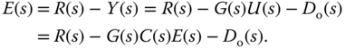
Therefore, the error signal is expressed as

(2.9)

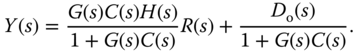
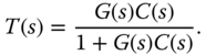
Then, the output of the control system is

(2.10)

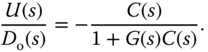
and the control signal is

(2.11)

Assuming that is zero, the transfer function between the reference signal and the plant output is

(2.12)

and the transfer function between the reference signal and the control signal is

(2.13)

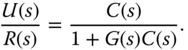
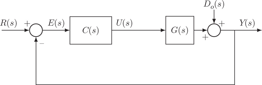
Figure 2.8 One degree of freedom control system structure.

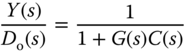
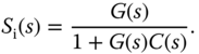
Similarly, by assuming , we derive the transfer functions between the output disturbance and the output, and the output disturbance and the control signal:

(2.14)

(2.15)

The properties of these closed-loop transfer functions are directly related to the closed-loop performance, determining the behavior of the output signal and the control signal in relation to reference signal and the output disturbance . In this controller structure, once the controller is selected, all four closed-loop transfer functions are fixed; only one degree of freedom is available to influence the output response to the reference signal and to the disturbance . This is called one degree of freedom design.

2.4.2 Two Degrees of Freedom Design

A two degrees of freedom control system is shown in Figure 2.9. In this structure, an extra component is placed after the reference signal , which will be used in the design. denotes the output disturbance, denotes the input disturbance, denotes the measurement noise. How does this structure offer two degrees of freedom in the design? For this, with the assumption that and , we calculate the output response in relation to the reference signal and the output disturbance ,

(2.16)

From this, we have the two transfer functions

(2.17)

(2.18)

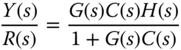
Transfer function provides one more degree of freedom to shape the output response to the reference signal . This extra degree of freedom plus the original one degree of freedom gives the two degrees of freedom in the design. If the control system is configured as a, then we can shape, independently, the output response to the reference signal and to the disturbance.

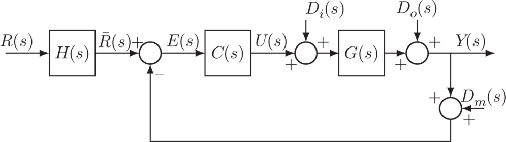
Figure 2.9 Two degrees of freedom control system structure.

Figure 2.10 Two degrees of freedom PI control system structure, where and .

2.4.2.1 Two degrees of freedom implementation of PI controllers

From Example 1.3, the IP controller structure illustrated in Figure 1.7 is in fact a two degrees of freedom implementation of a PI controller with a reference filter , where the reference filter is 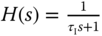, which is illustrated in Figure 2.10. One may argue that the choices of proportional controller gain and the integral time constant have cemented the characteristics of disturbance rejection; however, the value of has provided an extra degree of freedom to influence reference response. The advantage of using the IP controller is that the implementation procedure is simpler, because there is no need for the implementation of reference signal filter. In the general framework of two degrees of freedom controller implementation, may also be designed carefully to achieve desired effect of reference response.

2.4.3 Sensitivity Functions in Feedback Control

To understand the sensitivity functions and their roles in feedback control, we examine the block diagram of a closed-loop feedback control system illustrated in Figure 2.9.

Based on the block diagram, we calculate the feedback error of the closed-loop system firstly as

(2.19)

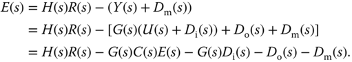
By re-arranging (2.19), the closed-loop feedback error is

(2.20)

Note that the feedback error is relation to the output via,

(2.21)

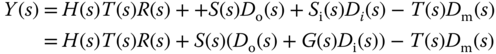
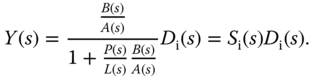
By substituting (2.21) into (2.20), we obtain the expression of the closed-loop output as

(2.22)

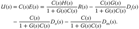
Also, from the feedback error (2.20), we calculate the closed-loop control signal as

(2.23)

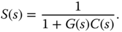
Based on these relationships, the following sensitivity functions are defined.

• Sensitivity function:
  
• Complementary sensitivity function:
  
• Input disturbance sensitivity function:
  
• Control sensitivity function:
  

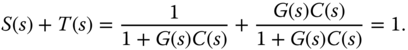
The sensitivity functions are related to each other in the following ways.

• The sensitivity plus complementary sensitivity is equal to one:
  (2.24)
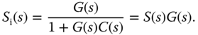
• The input disturbance sensitivity is related to sensitivity:
  (2.25)
• The control sensitivity is related to sensitivity:
  (2.26)

With the sensitivity functions, we re-write the output of the closed-loop system (2.22) as

(2.27)

and the control signal (2.23) as

(2.28)

From these relationships, we can see that:

1. The complementary sensitivity function represents the effect of both reference signal and measurement noise on the output.
2. The sensitivity represents the effect of output disturbance on the output.
3. The input sensitivity represents the effect of input disturbance on the output.

2.4.4 Food for Thought

1. In the two-degrees-of-freedom control system structure, must the reference filter be stable?
2. In many applications, instead of designing the reference filter, it is simpler to design the reference signal by deploying a ramp signal between two constant references. Assuming that at time , the reference signal , we would like the reference signal to be increased to 3 in a duration of 10 seconds. What does this reference signal look on a piece of paper? If you would like to duplicate this signal using the reference filter , what would you do?
3. Can you think of a reason why we would use the IP controller instead of using the two-degrees-of- freedom approach when we need to overcome the reference overshoot problem in PID control systems?
4. If the IP controller you designed still resulted in overshoot in reference response, what would you do?
5. With respect to PID control, by examining the closed-loop transfer function (1.40) in Example 1.4, which reference filter would you use to reduce the overshoot in the closed-loop step response caused by the derivation control?

2.5 Reference Following and Disturbance Rejection

Aside from stabilization of unstable systems, the two most important purposes that a feedback control system serves are reference following and disturbance rejection. In this section, we will discuss these two topics in relation to the complementary sensitivity and the sensitivity function . Their effects on the output will be measured and analyzed in the frequency domain. One caution is that closed-loop stability is a pre-requisite for the sensitivity analysis to be valid.

2.5.1 Closed-loop Bandwidth

For simplicity, we assume that to begin the discussion. From (2.27), the complementary sensitivity represents the effect of reference following on the output and the sensitivity represents the effect of disturbance rejection. Intuitively, for a control system designed with good reference following properties, we would like to see the complementary sensitivity so that the output for some designated frequencies, where is the frequency response of the reference signal. On the contrary, for disturbance rejection, intuitively, we would like the magnitude of the sensitivity function so that the output for some frequencies contained in the output disturbance signal or the input disturbance signal . As from (2.24), the sum of and is equal to one. Two observations follow immediately.

1. If at a given frequency , then .
2. Similarly, if is large, then is small.

This basically says that the control objectives for reference tracking or disturbance rejection using feedback can be achieved using the same qualitative and quantitative measure of either complementary sensitivity function or sensitivity function because . The implication is that if a feedback control system has a good tracking performance for a reference signal, then it will also have a good disturbance rejection for the disturbance signals that have the identical frequency characteristics. In other words, the reference following and disturbance rejection in feedback control share the same goals in the design without conflicting.

We can also examine the reference tracking from feedback error analysis to reach the same conclusions as above. Consider a unit negative feedback control system with the reference pre-compensation . The feedback error signal is simply computed as

(2.29)

It is seen here that, for the reference tracking, the feedback error is directly related to the sensitivity function . Therefore, if is small over some frequency band, then the feedback control system will yield, on the same frequency band, better reference tracking as well as disturbance rejection performance. This re-iterates that the control system design objectives for reference following and disturbance rejection share the same characteristics over either the complementary sensitivity or the sensitivity function.

One of the qualitative measures in sensitivity analysis is the characterization of closed-loop bandwidth . The parameter bandwidth is a frequency parameter either in the unit of Hertz (Hz) or , which corresponds to the frequency when the complementary sensitivity function has the following value:

As illustrated in Figure 2.11, the magnitude of a complementary sensitivity function is intersected with a dash-dotted horizontal line with a value of , where the vertical dash-dotted line leads to the bandwidth of . As demonstrated in Section 2.3, one can easily use the MATLAB ginput.m function to identify the bandwidth from the plot of the complementary sensitivity function by putting the hair cross line at the point when the dash-dotted line intersects the magnitude of complementary sensitivity. For reference following, the bandwidth is interpreted as if the frequencies of the reference signal fall between 0 and , then the output signal will have the capacity to closely duplicate this reference signal. For disturbance rejection, because is small between 0 and , if the frequencies of a disturbance signal fall into this range, then the output will have the capacity to suppress the disturbance.

Having said that minimization of the effect of disturbance will certainly lead to maximizing tracking performance of the same type of reference signals, in engineering applications there might be additional constraints on the reference tracking such as output overshoot of the reference signal. The two degrees of freedom control system implementation provides an additional means in an open-loop manner to shape the reference tracking properties by selecting the stable reference filter .

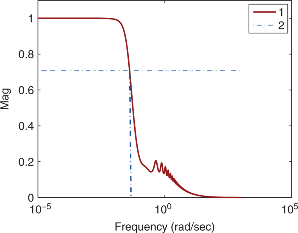
Figure 2.11 Complementary sensitivity function with bandwidth illustration. Key: solid line: ; dash-dotted lines: illustration of bandwidth.

One exception to the shared common ground of disturbance rejection and reference following is the scenario when there is pole-zero cancellation in the controller structure. Pole-zero cancellation is a commonly used technique for control system design because it simplifies the controller parameter solutions. Assuming that the controller transfer function is and the model transfer function is from Figure 2.9, with , the output response to the reference signal is

(2.30)

and to the input disturbance is

(2.31)

Note that in the complementary sensitivity function , and appear in pairs. Therefore, the poles or zeros that have been canceled in the design will disappear from the complementary sensitivity function, meaning that they will not affect the closed-loop performance of reference tracking. However, in the input disturbance sensitivity function , and appear in pairs only for the denominator. Thus, if a pole from the system transfer function is canceled in the controller design, it will re-appear as the same pole in the input disturbance sensitivity function because does not appear in the numerator. This means that if a system pole is canceled in the controller structure, a fast reference following response does not automatically imply a fast input disturbance rejection, depending on the location of the canceled pole. A detailed study of pole-zero cancellation on the effect of disturbance rejection is given in Example 3.7.

2.5.2 Reference Following and Disturbance Rejection with PID Controllers

PID controllers are the most widely used controllers in engineering applications. Their successful applications are aligned with the most commonly encountered reference signals and disturbance signals. The reference signals for PID controller applications are a step signal or a series of step signals. For instance, if we want to regulate a room temperature to C from the current temperature of C, then the reference signal is a step signal with amplitude of C. In other words, the output of a PID control system is regulated to a constant value. Note that the Laplace transform of a unit step signal is with the magnitude of frequency response 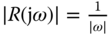, which is infinity at . Hence, for the output to follow a step reference signal perfectly, the complementary sensitivity function at the zero frequency. This automatically implies that the sensitivity function , which is required for tracking the step reference signal and rejecting a disturbance with its frequency contents concentrated at the zero frequency.

Now, on a back envelope calculation, if the plant model does not contain a zero at , the integrator contained in a PID controller will simultaneously yield and because the integrator in the controller creates an infinite gain for the loop transfer function 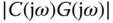at . The sensitivity function contains a zero at as long as the plant model does not contain a zero at .

Because the majority of the control systems are designed to track a constant reference signal or regulate the output to a constant value, additionally, the most disturbances occurred in the process control applications are rich in the low frequency region, the PID controllers are adequate for the commonly encountered applications.

---

Example 2.4

Consider the first order plus time delay system described by the transfer function

Use the Padula and Visioli tuning rules (Padula and Visioli (2011)) to determine the PID controller parameters with consideration of two cases: and , and analyze their properties for reference following and disturbance rejection using the complementary sensitivity and sensitivity functions .

Solution. Using the Padula and Visioli tuning rules presented in Table 1.5, we find two sets of PID controller parameters. For , we have

and for , we have

Because there is a derivative filter used in the PID controller, the controller transfer function becomes

where the derivative filter time constant is taken as .

Figure 2.12 Nyquist diagrams using Padula and Visioli PID controller (Example 2.4). Key: line (1) ; line (2) .

Firstly, we verify closed-loop stability of the two PID controlled systems by plotting their Nyquist diagrams shown in Figure 2.12. It is seen that the PID controllers produce sufficient gain margins and phase margins.

Next, we present the magnitudes of the complementary sensitivity functions in Figure 2.13 with illustration of the bandwidth. They are equal to 0.0403 and 0.0657 , respectively. The bandwidth of the PID controller tuned using the is larger among the two cases. The magnitudes of the sensitivity functions are presented in Figure 2.14. It is interesting to note that the sensitivity peak for the case is close to the specification. However, for the case, the sensitivity peak is less than the specified value of 2, but it is higher than that obtained in the previous case.

To simulate the closed-loop response for reference following and disturbance rejection, we use the two degrees of freedom PID implementation to avoid overshoot in output when the reference signal is a unit step, where both the proportional control and the derivative control are implemented on the output only. By selecting the sampling interval s, the closed-loop simulation is performed with a unit step signal for the reference and a step input disturbance with unknown amplitude entering the system at half of the simulation time. Figure 2.15(a) shows the closed-loop control signals for the reference following and disturbance rejection. It is seen that for the tuning rule with , the control amplitude variations are larger. Figure 2.15(b) shows the closed-loop output response. It confirms that the output from the tuning rule with is faster among the two responses. The time domain performances are consistent with the frequency response analysis that the PID control system with the wider bandwidth produces a faster reference tracking as well as disturbance rejection. It is worthwhile mentioning that the two degrees of freedom implementation is crucial to reduce the overshoot for the reference change when using the tuning rules produced by Padula and Visioli. As an exercise, one is encouraged to implement the one degree of freedom PID controller and observe the substantial amount of overshoot occurring in the closed-loop step response for the reference change.

Figure 2.13 Complementary sensitivity function using the Padula and Visioli PID controller with bandwidth illustration. Key: line (1) ; line (2) .

Figure 2.14 Sensitivity function using the Padula and Visioli PID controller. Key: line (1) ; line (2) .

Figure 2.15 Comparison of closed-loop responses using Padula and Visioli PID controller (Example 2.4). (a) Control signal. (b) Output. Key: line (1) tuning rule with ; line (2) tuning rule with .

---

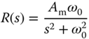
2.5.3 Reference Following and Disturbance Rejection with Resonant Controllers

In the applications of control systems to power electronics, aerospace, and mechanical engineering, it is often required for the output of the closed-loop control system to track sinusoidal reference signal or to reject a sinusoidal disturbance. In these applications, we assume that the sinusoidal reference signal is with known parameters. However, for disturbance rejection, the disturbance signal is expressed as 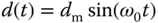, where the frequency is known but the amplitude of the disturbance is unknown.

Note that the Laplace transform of the reference sinusoidal signal with frequency is

with frequency response

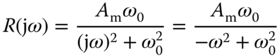
Thus, as , .

From the sensitivity analysis, in order for the feedback control system to have a good tracking performance for the sinusoidal reference signal, we need the complementary sensitivity function at . Similarly, to reject the sinusoidal disturbance signal with unknown amplitude, we need to have the sensitivity function at . In order to achieve these characteristics for the feedback control system, a quick calculation indicates that the feedback controller is required to embed the mode into its structure, assuming that the plant does not contain a pair of complex zeros at . In the literature, this type of controller is called either resonant controller or repetitive controller because of the periodic nature of the external signals.

We consider the case that is a multi-frequency periodic signal, defined as where the frequencies , and are given. In order to track this multi-frequency periodic signal using a feedback controller, the complementary sensitivity function is required to satisfy at the frequencies . As a result, the sensitivity function automatically satisfies at the frequencies . Therefore, the controller designed for following the multi-frequency periodic reference signal will also reject a periodic disturbance with the same frequencies. The controller is required to embed the following components

into its structure in order to achieve or at the frequencies . Here we need to assume that the plant does not have complex zeros at the corresponding frequencies.

In Section 3.5, pole-assignment controller design techniques will be introduced for the design of resonant controller. In Section 5.4, a resonant controller will be designed using a disturbance estimation technique together with anti-windup implementation. This disturbance estimation based design technique is extended to a multi-frequency sinusoidal reference/disturbance signal in Section 5.5.

2.5.4 Food for Thought

1. If the disturbance rejection is too slow, taking a long time for the output response to recover, would you decrease the closed-loop bandwidth?
2. For a PID controlled system with , and , if the bandwidth were too small, would you increase ?
3. For the IMC-PID tuning rules (see Section 1.4.1), the original tuning-rules (Equation (1.47)) will lead to a slow response to input disturbance. Can you explain this using the characteristics of the input sensitivity function?
4. Why is the two-degrees-of-freedom PID controller implementation important in the context of reference following and disturbance rejection?
5. In many applications, rejecting load disturbance is the primary objective of the control systems. Load disturbance is often modelled as a constant input disturbance. To avoid a large disruption to the system when switching on a load is paramount. How can we design such a load profile so that it can be switched gradually?

2.6 Disturbance Rejection and Noise Attenuation

Both noise and disturbance co-exist in a physical system. A good closed-loop performance requires minimization of the effects of both disturbance and noise.

2.6.1 Conflict between Disturbance Rejection and Noise Attenuation

For minimization of the effects of both input and output disturbances, we make the magnitude of the output in frequency response

(2.32)

as small as possible. For minimization of the measurement noise, we make the magnitude of the output in frequency response

(2.33)

as small as possible, indicating that there is a conflict between disturbance rejection and noise attenuation.

We cannot alter the disturbances and noise because they already existed in the system. Thus, what we do is to make:

• the magnitude of sensitivity () small for disturbance rejection;
• the magnitude of complementary sensitivity () small for noise attenuation.

These are the basic design principles for control systems. However, noting that the relationship between the sensitivity and complementary sensitivity is constrained by

(2.34)

which says that we cannot make both and small over the same frequency bands. In other words, if the disturbance is minimized in a given frequency region where is small, then inevitably the measurement noise is not attenuated in the same frequency region where is large. So how are we going to design a closed-loop control system that will minimize the effects of disturbance and the measurement noise?

Note that the disturbances existing in the system correspond to slow movement of the variables or slow changes, therefore the frequency contents of the disturbance term are concentrated in the low frequency region. In contrast, the measurement noise corresponds to fast movement of the variables or fast and frequent changes of the variables, therefore the frequency contents of the measurement noise are concentrated in the higher frequency region. This means that we can achieve disturbance rejection by choosing the sensitivity function at the low frequency region, which implies at the low frequency region, because . This is not too bad for noise attenuation because is small in the low frequency region. At the high frequency region, to avoid the amplification of measurement noise, we choose , which implies . This is not too bad for disturbance rejection because is small in the high frequency region. In short, to achieve a trade-off relationship between disturbance rejection and noise attenuation, a closed-loop bandwidth should be carefully selected.

2.6.2 PID Controller for Disturbance Rejection and Noise Attenuation

Two examples are given in this section to illustrate the relationship between disturbance rejection and noise attenuation when using a PID controller.

---

Example 2.5

Consider the transfer function model given in Ralhan and Badgwell (2000) to describe the operations of a gas fired heater at a low fuel operation:

(2.35)

This transfer function was approximated using the first order plus delay model in Section 1.5.2 as

(2.36)

Use the Padula and Visioli tuning rules to determine the PID controller parameters for the fired heater system, and evaluate the PID controllers' performance in disturbance rejection and noise attenuation.

Solution. For the PID controller tuning rule that corresponds to , use of Table 1.5 together with the first order approximate model (2.36) leads to the following PID controller parameters:

The PID controller parameters corresponding to the sensitivity peak are

Figure 2.16 Nyquist diagrams using the Padula and Visioli PID controller (Example 2.5). Key: line (1) ; line (2) .

We evaluate the closed-loop stability by finding the Nyquist loci of the PID controllers with the plant model (2.35) where the derivative filter time constant is selected as . As shown in Figure 2.16, the point is not encircled, thus both PID control systems are stable with sufficient gain and phase margins. To evaluate the closed-loop performance for disturbance rejection, we examine the magnitude of the sensitivity functions (see Figure 2.17(a)). It is seen that is smaller for the design corresponding to in the lower frequency region; however, it becomes very large in the medium frequency region with a peak greater than 2. We can conclude that the PID controller corresponding to will have better disturbance suppression in the lower frequency region, however the performance will dramatically decay when the disturbance frequency increases to the medium to higher frequency region.

To evaluate the closed-loop performance for noise attenuation, we examine the magnitude of the complementary sensitivity function (see Figure 2.17(b)). It is seen that the complementary sensitivity for the PID controller with has a large spike at the medium frequency region, also its magnitude is larger at the higher frequency region. It is concluded that the PID controller with is more sensitive to noise. Closed-loop simulation is used to evaluate the time domain responses for disturbance rejection and noise attenuation. The sampling interval is selected to be 1 s. A unit input step disturbance enters the closed-loop control system at half of the simulation time and there is a measurement noise with variance 0.01 added to the simulation. Figures 2.18(a) and (b) compare the closed-loop control signal responses to the disturbance and measurement noise. It is indeed seen that the control signal for the case is more sensitive to the noise. By comparing the output responses (see Figures 2.18(c) and (d)), we find that the output response to the input disturbance is faster for the case that .

Figure 2.17 Sensitivity functions using Padula and Visioli PID controller (Example 2.5). (a) Sensitivity. (b) Complementary sensitivity. Key: line (1) ; line (2) .

Figure 2.18 Closed-loop responses to disturbance and measurement noise using Padula and Visioli PID controller (Example 2.5). (a) Control (). (b) Control (). (c) Output (). (d) Output ().

---

A derivative filter plays an important role in noise attenuation for a PID controlled system because the derivative action will amplify the measurement noise. The following example is used to show its significance in the presence of measurement noise in conjunction with the choice of sampling interval in the implementation.

---

Example 2.6

To emphasize that a derivative filter is paramount in the application of PID controllers, we continue from Example 2.5 by examining how the filter time constant affects the noise attenuation in the closed-loop system. In the implementation of a PID controller, we will reduce the filter time constant from to and reduce the sampling interval accordingly. We leave the sensitivity function analysis as an exercise, instead we will present the simulation studies.

Figure 2.19 Closed-loop responses to disturbance and measurement noise using Padula and Visioli PID controller (Example 2.6). (a) Control (). (b) Control (). (c) Output (). (d) Output ().

Solution. With the filter time constant reduced, the sampling interval needs to be reduced accordingly to avoid numerical instability in the simulation. In this simulation, is reduced from 1 to 0.1. With the identical input disturbance and noise amplitude, the closed-loop response is simulated for disturbance rejection and noise attenuation. From Figures 2.19(a) and (b), it is seen that the control signal is completely distorted by the noise, although the output is less distorted. The main cause of the noise amplification is because the derivative term is particularly sensitive to the reduction of the filter time constant. Since the PID controller is designed in continuous time, a smaller sampling interval is required for a smaller time constant from the derivative filter.

---

2.6.3 Food for Thought

1. Would you increase the bandwidth of the closed-loop control system if a low quality sensor is used in the measurement device and the measurement noise is severe?
2. When using a resonant controller, if the frequency embedded into the controller is large, would you expect that the measurement noise will be amplified more than that with a PID controller?
3. In the implementation of PID controller, if the measurement noise is severe, would you decrease the derivative filter time constant?
4. Would you prefer to use a PI controller instead of a PID controller if the noise is severe?

2.7 Robust Stability and Robust Performance

Robust stability and robust performance are two important issues for a control engineer to consider when a feedback control system is designed and to be implemented. The phrase “robust control” is used to imply that the control system designed can withstand the uncertainties caused by the discrepancies between the model used for the controller design and the actual plant model.

2.7.1 Modeling Errors

Many of us, as a control engineers, have experienced a feedback control system designed using the correct methodologies and the closed-loop simulation has yielded satisfactory performance; however, the control system failed to produce stable closed-loop operation when it was implemented. More than often, the key reason behind the discrepancy between what is desired and what is reality is the existence of modeling errors between the model used for the control system design and the behavior of the actual system at specific operation conditions.

There are a few factors causing the existence of modeling errors in control system design depending on how the mathematical model is derived. In electrical engineering applications, such as electrical machine control and power converter control, the mathematical models are derived from physical laws using current and voltage (see Wang et al. (2015)). Similarly physical laws are used to derive the mathematical models for electro-mechanical systems such as unmanned aerial vehicles (see Chapter 10), and ball and plate balancing systems (see Chapter 6). The mathematical models derived using physical laws are referred mechanistical models, which are often in the form of nonlinear differential equations (see Chapter 6). The modeling errors for the electrical systems and the electro-mechanical systems are often caused by an inaccurate measurement of the physical parameters and the variations of the operating conditions.

In chemical process control applications, due to the lack of clearly defined physical laws or the complexities of the physical systems, the mathematical models are commonly obtained by directly conducting identification experiments on the plant and estimating a transfer function model based on the input and output measurement data (see the fired heater system (Ralhan and Badgwell (2000)) in Section 1.5.2). The mathematical models derived using the identification experiments (see Chapter 9) are referred empirical models. The modeling errors for the chemical process control applications are often caused by restricted identification experimental conditions including small input signal amplitude, corruptions of large measurement noise and disturbances, model estimation errors, as well as variations of operating conditions.

Furthermore, when using a restricted controller structure such as a PID controller, the mathematical models could be too complex for the design of a simple controller. Thus, model order reduction is required, which leads to another source of modeling errors. In the context of control system design, there is an unknown transfer function denoted by , which accurately describes the linear time invariant system at a given operating condition. However, for the various reasons discussed above, this is seldom available to us. Instead, a transfer function model is obtained from linearization (see Chapter 6) or from identification experiments and used in the control system design. This leads to the conceptual description of modeling errors that consist of the following forms in the literature:

(2.37)

(2.38)

where is called the additive modeling error and is called the multiplicative modeling error. We assume that the modeling errors are stable.

Except that in the case of model order reduction for PID controller design, is assumed unknown, thus the exact descriptions of and may not be available. However, in robust control, it is often that the bounds on the frequency responses are used to quantify the impact of the modeling errors, for ,

(2.39)

(2.40)

In a simplified case, the modeling error bound may be chosen as a constant, which produces a conservative measure for the modeling errors.

2.7.2 Robust Stability

Robust stability for a control system is quantified and analyzed in the frequency domain in terms of the additive and multiplicative modeling errors defined, with its origin from the Nyquist stability criterion introduced in Section 2.3. The purpose is to assess closed-loop stability when the controller is applied to the unknown system .

To start, we consider that the open-loop system is stable and assume the following conditions are satisfied.

• The controller is designed to stabilize the model with all closed-loop poles strictly on the left half of the complex plane.
• The modeling errors, either additive or multiplicative, are stable.

Then, from the Nyquist stability criterion, the necessary and sufficient condition for closed-loop stability when the controller is applied to the unknown system is that the frequency response of the loop transfer function will not encircle the point on the complex plane. This is translated into the following inequality:

(2.41)

for all . Because is unknown, in Equation 2.41 it is replaced by the model and the additive modeling error , leading to

(2.42)

which is

(2.43)

Now, since the controller is designed to stabilize the model , the Nyquist loci of will not encircle the point, it ensures that

for all .

Therefore, the inequality (2.41) is satisfied if

Or, more conservatively, for all ,

This leads to the robust stability condition in the frequency domain as

(2.44)

for all . This robust stability condition is a sufficient condition, which ensures the Nyquist loci of the not to encircle the point through the representation of additive modeling error.

The robust stability condition (2.44) can also be written in terms of the multiplicative modeling error by noting that

leading to

(2.45)

With the multiplicative modeling error, the robust stability condition is expressed in relation to the complementary sensitivity function .

With the frequency response bound defined as in (2.39), the robust stability condition becomes:

(2.46)

for all . Alternatively, with the multiplicative modeling error bound defined in (2.40), it has the following representation:

(2.47)

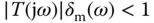
for all .

The first robust stability condition (2.46) is expressed in terms of the control sensitivity function whilst the second stability condition (2.47) is expressed in terms of the complementary sensitivity function, which is directly related to the closed-loop control performance specifications.

The robust stability condition (2.47) says that if the multiplicative modeling error is larger than 1 at a given frequency , then needs to be less than 1 to ensure closed-loop stability. Conversely, if is large at a certain frequency region, then a small modeling error is required in the same region to ensure closed-loop stability. Clearly, if the controller contains an integrator, then , which indicates that in order to guarantee closed-loop stability. Similarly, for the resonant controller that has embedded a sinusoidal mode at , , leading to the condition that in order to guarantee robust closed-loop stability.

In summary, the existence of modeling error gives an additional constraint on the complementary sensitivity function. This constraint is translated into the selection of the desired closed-loop bandwidth as demonstrated in the following case study.

2.7.3 Case Study: Robust Control of Polymer Reactor

---

Example 2.7

The mathematical model for the eighth reactor in a copolymerization reactor train is described by the following transfer function model (Madhuranthakam and Penlidis (2016)):

(2.48)

where the input is the flow rate of the chain transfer agent (CTA) to the first reactor in the reactor train and the output is the weight-based average molecular weight (). The parameters in the transfer function for the reactor are given as , and .

For this case study, we will perform the following tasks.

1. We will find the first order plus delay approximate model using the step response data, and calculate the additive and multiplicative modeling errors.
2. Based on the IMC-PI controller tuning method, by choosing , which is the time delay of the first order approximate model, we will calculate the PI controller parameters and check if the closed-loop system is robustly stable. As a comparison, we will increase to in order to observe its effect on the robustness of the control system.

Solution. With sampling interval s, the unit step response of the transfer function (2.48) is calculated as shown in Figure 2.20. Clearly, it is seen that the steady-state gain is 1 and the system has a large time delay.

By drawing a line to produce a maximum slope, which is then intersected with the steady-state line as shown in Figure 2.20, the time delay for this reactor is estimated as 128.5 (min) and the time constant is 168.5 (min). This graphic approach leads to the first order plus time delay model as

Figure 2.20 Unit step response of the eighth reactor with lines to assist obtaining first order plus delay model.

(2.49)

The additive modeling error is calculated as

and the multiplicative modeling error is

Because the reactor's transfer function model has eight stable zeros, which becomes a large lead element in the dynamic response and has been neglected in the first order plus delay model, there is a large discrepancy between the system and the approximate model. This large discrepancy is reflected in the magnitudes of the frequency response of the modeling error both additive and multiplicative, as shown in Figures 2.21(a) and (b). In particular, the magnitude of exceeds 3 at . This indicates that the desired bandwidth of the closed-loop control system needs to be quite small in order to guarantee closed-loop stability in the presence of a modeling error.

Figure 2.21 Magnitude of modeling errors with the first order plus delay model (Example 2.7). (a) Additive modeling error. (b) Multiplicative modeling error.

For systems with a large time delay, the desired time constant is commonly selected to be larger than the time delay. We will start by choosing the desired time constant (min), which leads to

(2.50)

where , and . It can be checked using a Nyquist plot that this PI controller will lead to a stable closed-loop system when it is used to control the first order plus time delay model (2.49). So we check if the robust stability condition (2.47) with respect to the multiplicative modeling error is satisfied. Figure 2.22(a) shows the magnitude of the complementary sensitivity function. With the choice of , the magnitude of the complementary sensitivity decays rapidly (see the solid line), and as a result the robust stability condition is satisfied where the quantity is less than 1. Therefore, we can conclude that the IMC-PI controller will produce a stable closed-loop system for the polymer reactor model based on (2.48) when . As a comparison, we increase the desired closed-loop time constant to . Figures 2.22(a) and (b) show the further reductions of the magnitude of the complementary sensitivity function and the quantity . Finally, the performance of the closed-loop control system is evaluated against the transfer function model (2.48) with the proportional control implemented on the output only. Figures 2.23(a) and (b) show the closed-loop step response of the control signal and output signal respectively. It is seen that when , the closed-loop responses are severely oscillatory, however when is increased to , the oscillation is almost overcome. In summary, increasing the desired closed-loop time constant , which essentially reduces the desired closed-loop bandwidth, will enhance the robustness of the control system when the plant is stable.

Figure 2.22 Complementary sensitivity function and graphic presentation of robust stability condition (Example 2.7). (a) Magnitude of complementary sensitivity function. (b) . Key: line (1) ; line (2) .

Figure 2.23 Closed-loop step responses (Example 2.7). (a) Control. (b) Output. Key: line (1) ; line (2) .

This process is to be studied again as an exercise (see Problem 8.3) using the frequency response design technique introduced in Chapter 8, where closed-loop control performance improvement is expected.

---

Note that many of the empirical tuning rules for PID controllers do not have a performance tuning parameter to adjust the desired closed-loop performance in order to account for the modeling errors. This is the biggest limitation for the empirical PID controller tuning rules. For the IMC-PID controller, the desired closed-loop bandwidth is selected by adjusting the desired closed-loop time constant .

2.7.4 Food for Thought

1. If we neglected a time delay in the design, what would be the multiplicative modelling error?
2. If the Padula and Visioli PID controller tuning rules produced an unstable closed-loop system, would you try to reduce the proportional control gain or increase the integral time constant ?
3. Is it correct to say that the modelling error limits the closed-loop bandwidth?
4. Is it correct to say that in general we need a model with higher accuracy for a higher demand in the closed-loop performance for disturbance rejection and reference following?

2.8 Summary

In this chapter, we have presented the commonly used tools for closed-loop stability and performance analysis. Understanding the relationships between the closed-loop poles, closed-loop stability, and performance is crucial in control system design and analysis. In the later chapters, we will discuss model based controller design methods that specifically use the locations of the desired closed-loop poles as performance specification. The important aspects discussed in this chapter are:

• If the closed-loop transfer function is known with constant coefficients, then the closed-loop poles can be simply determined by finding the solutions of the characteristic equation. Numerically, this is achieved using MATLAB function root.m for the denominator of the transfer function.
• The Routh-Hurwitz stability criterion explicitly determines whether a closed-loop system is stable by examining the coefficients of the closed-loop characteristic polynomial. This is particularly useful when we need to determine the effect of the variation of a parameter on the closed-loop system.
• Nyquist stability criterion is based on the frequency response of the open-loop transfer function that includes the system, the controller, the actuator and the sensor. It involves the presentation of the frequency response graphically with real and imaginary parts (a two dimensional plot), revealing the important quantities such as gain margin, phase margin and delay margin. Because it is based on the frequency domain, time delay in the system can be easily captured.
• Sensitivity analysis based on the frequency domain is fundamental to the understanding of the characteristics of closed-loop control systems. In the context of sensitivity analysis, the parameter called closed-loop bandwidth is defined.
• Understanding the closed-loop performance in terms of disturbance rejection and reference following is based on the frequency response of the sensitivity function and complementary sensitivity function. Because the relationship between the complementary sensitivity function and sensitivity function is captured by:
  
  the performance requirements are consistent in the sense that a closed-loop system that has a fast reference following will also have a fast disturbance rejection.
• Understanding the closed-loop performance in terms of disturbance rejection (or reference following) and measurement noise attenuation is also based on the frequency response of the sensitivity function and complementary sensitivity function. However, the relationship
  
  captures the fundamental trade-off between disturbance rejection and measurement noise attenuation. There is a conflict between the two requirements, meaning that a fast disturbance rejection in a closed-loop control system will inevitably lead to the amplification of measurement noise. The existence of measurement noise limits the closed-loop control performance in terms of disturbance rejection and reference following.
• Modelling errors are often present in the PID control system design. Because of their existence, there is a difference in the closed-loop performance between what is desired and what is actually achieved. Their effects on the closed-loop performance are analyzed and quantified in the frequency domain using the errors and the complementary sensitivity function. Furthermore, the Nyquist stability criterion provides an effective means to access the information about gain margin, phase margin and delay margin, which are important to assess the impact of modelling errors on closed-loop stability.

2.9 Further Reading

1. Text books in control engineering include, Franklin et al. (1998), Franklin et al. (1991), Ogata (2002), Golnaraghi and Kuo (2010), Goodwin et al. (2000) and Astrom and Murray (2008).
2. Disturbance rejection, reference following and robustness are discussed in Garpinger et al. (2014), in Alcántara et al. (2013). Two-degrees-of-freedom PID controller design is proposed in Gorez (2003) and Yukitomo et al. (2004), Araki and Taguchi (2003). Load disturbance rejection with consideration on robustness of closed-loop system is proposed in Panagopoulos et al. (2002). Effect of noise for tuning the controller parameters is discussed in Fertik (1975).
3. The Ziegler-Nichols step response method is revisited from the point of view of robust loop shaping in Åström and Hägglund (2004).
4. Tuning of PID controllers based on gain and phase margin specifications was proposed in Ho et al. (1995), Ho and Xu (1998), Ho et al. (2000). The Ziegler-Nichols, and Cohen-Coon tuning formulas that optimize for load disturbance response are analyzed in Ho et al. (1996) for gain margin and phase margin. Gain and phase margins are used in selecting PID controller parameters with consideration of robustness and closed-loop performance in Ho et al. (1998).
5. Disturbance rejection for the modified IMC tuning rules is specifically addressed in Skogestad (2006). Robustness of IMC is discussed in Morari and Zafiriou (1989). Further discussions of tuning guidelines and robustness for IMC can be found in Vilanova (2008).

Problems

1. 2.1 In Example 2.3, three PI controllers (see Table 2.3) were found using tuning-rules together with analysis of Nyquist diagram for the following continuous-time system:
   (2.51)
   1. Evaluate the closed-loop step response of the three PI control systems in one-degree-of-freedom using a Simulink simulation.
   2. Evaluate the closed-loop step response of the PI control systems in two-degrees-of-freedom where the reference filter is selected as , and compare the output responses with the simulation results presented in Figure 2.7.
2. 2.2 In Example 1.8, Padula and Visioli tuning rules were used to find PID controller for the following system
   

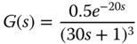
   where , , .

   1. Find the closed-loop transfer function between and with the control signal defined as
      

      Simulate the closed-loop unit step response for this one-degree-of-freedom control system with sampling interval (sec).

   2. Find the closed-loop transfer function between and with the control signal defined as
      

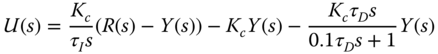
      Simulate the closed-loop step response for this IPD control system and compare the results with the ones from the one-degree-of-freedom controller structure.

   3. Observing from the closed-loop transfer functions, what reference filter should be chosen if the remainder of the overshoot from the IPD implementation were to be eliminated? Verify the results using the selected reference filter.
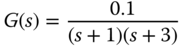
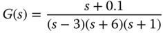
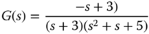
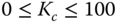
3. 2.3 Use Routh-Hurwitz stability criterion to determine the range of the proportional controller that will stabilize the systems with the following transfer functions.
   1. 
   2. 
   3. 
   4. 
4. 2.4 Use Routh-Hurwitz criterion to determine the range of the integral time constant that will produce a stable closed-loop system for the plant with transfer function . Here we assume that the proportional gain .
5. 2.5 Consider a system with the following transfer function:
   
   1. Assuming that the integral time constant , form the closed-loop characteristic equation in terms of the proportional control , and numerically determine the variations of closed-loop poles with respect to (). This numerical procedure leads to root-locus analysis of the PI control system with respect to the variations of .
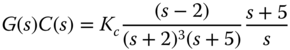
   2. Alternatively, we can use MATLAB function ‘rlocus.m’ for the root-locus analysis with the loop transfer function:
      
   3. From the root-locus analysis, determine the range of the proportional gain that will produce a stable closed-loop system.
   4. What are your observations on the closed-loop pole variations with respect to the proportional gain from the root-locus analysis?
6. 2.6 This Problem is an extension to Example 2.7. Because the reactor's transfer function model has 8 stable zeros, it is difficult to design a PID controller using the PID tuning rules without desired closed-loop performance adjustment.
   1. Use Padula and Visioli PID controller tuning rules based on the first order plus delay model shown in (2.49) to find two sets of PID controller parameters for and (see Table 1.5).
   2. Plot the Nyquist diagrams for both PID controlled systems using the original reactor model (2.48) and verify if the closed-loop systems are stable.
   3. Based on the Nyquist diagrams, propose what we would do to improve the gain margin and phase margin for the two PID controlled systems, and modify the PID controller parameters accordingly.
   4. Simulate the closed-loop step response for both systems based on the original reactor model (2.48) using the modified PID controllers.
7. 2.7 One of the simple and yet effective approaches to model order reduction is to neglect the small time constant in the transfer function model:
   

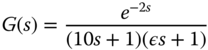
   in order to obtain a first order plus delay model.

   1. Determine the multiplicative modelling error when the approximate model is taken as .
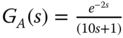   2. Calculate for and compare their magnitudes in a diagram. What are your observations?
   3. Use Padula and Visioli PID controller tuning rules () based on the first order plus delay model to find two sets of PID controller parameters.
   4. Calculate the complementary sensitivity function for the PID controller.
   5. Determine the closed-loop robust stability using the relationship
      

      for all . Is the closed-loop system stable for ?

   6. Compare the closed-loop step responses, which are simulated based on the original second order plus delay model for and with sampling interval and derivative filter time constant equal to . What are your observations?
8. 2.8 The original IMC-PI tuning rules are given for a first order plus delay system:
   

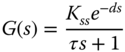
   where is the desired closed-loop time constant and

   (2.52)
   1. Find the complementary sensitivity function , the input disturbance sensitivity function for the IMC-PI controlled system. What are your observations in terms of the poles of the sensitivity functions?
   2. For a system with , , , calculate and for . Will change with respect to ? If so, what are the bandwidth parameters? Will change with respect to ?
   3. Simulate the closed-loop step response for the two PI controlled systems with sampling interval . Does affect the closed-loop step response speed?
   4. Simulate the closed-loop input disturbance response for the two PI controlled systems, where the disturbance is a constant with magnitude of 3. Does affect the closed-loop disturbance rejection?
   5. What if the disturbance occurred at the output, would make a difference on the disturbance rejection? Verify your intuition with the closed-loop simulation of output disturbance.