1
Basics of PID Control
1.1 Introduction
This chapter will introduce the basic ideas of PID control systems. It starts with an introduction to the roles of proportional control, integral control, and derivative control, followed by an introduction to the various tuning rules developed over the past several decades. These tuning rules are mainly developed for first order plus delay systems and are simple to use. However, they do not, in general, guarantee satisfactory control system performance. Simulation examples will be used to illustrate closed-loop performance.
This chapter is suitable for those who want to understand the very basics of PID control systems. By utilization of the tuning rules, it is possible to have an application of a PID control system without further exploration.
1.2 PID Controller Structure
There are four types of controllers that belong to the family of PID controllers: the proportional (P) controller, the proportional plus integral (PI) controller, the proportional plus derivative (PD) controller and the proportional plus integral plus derivative (PID) controller. To understand the roles of the controllers, in this section we will discuss each of the structures and the PID controller parameters. From the discussions, we will establish some basic knowledge about how to use these controllers in various applications.
1.2.1 Proportional Controller
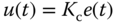
The simplest controller is the proportional controller. With this term proportional, the feedback control signal  is computed in proportion to the feedback error
  with the formula,
where  is the proportional gain and the feedback error is the difference between the reference signal
  and the output signal
  (
( ). The block diagram for the closed-loop feedback control configuration is shown in Figure 1.1 where
  ,
,  ,
,  , and
, and  are the Laplace transforms of the reference signal, feedback error, control signal, and output signal, respectively.
  represents the Laplace transfer function of the plant.

Figure 1.1 Proportional feedback control system.
Because of its simplicity, the proportional controller is often used in the cases when little information about the system is available and the required control performance in steady-state operation is not demanding. As the controller only involves one parameter to be determined, it is possible to choose  without detailed information about the plant.
One of the limitations of a simple proportional controller is that the steady-state error of the closed-loop control system will not be completely eliminated. We illustrate this point with the following example.
1.2.2 Proportional Plus Derivative Controller
In many applications, a proportional controller  is not sufficient to achieve a particular control objective such as stabilization or producing adequate damping for the closed-loop system. For instance, for a double integrator system with the transfer function:

the closed-loop control system with a proportional controller  has a transfer function

which has a pair of closed-loop poles determined by the solutions of the polynomial equation:

These poles are at  . Thus, no matter what choice we make for
  , the system still behaves in a sustained oscillatory manner because the pair of closed-loop poles are on the imaginary axis of the complex plane.
Now, assuming that we will additionally take the derivative of the feedback error signal into the control signal calculation, this leads to
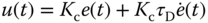
where  is the derivative control gain.
The Laplace transfer function of (1.8) is calculated as
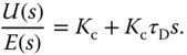
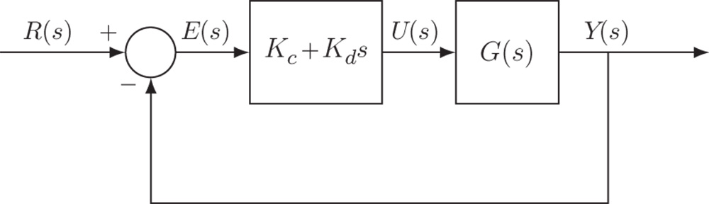
Figure 1.3 Proportional plus derivative feedback control system ( ).
).
This is what we called a proportional plus derivative (PD) controller.
The closed-loop feedback control configuration for a PD controller is shown in Figure 1.3. For the double integrator system (1.7), with the derivative term included in the controller, then the closed-loop transfer function becomes

The closed-loop poles are determined by the solutions of the characteristic polynomial equation as

which are
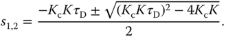
Clearly, we can choose the values of  and
and  to achieve the desired closed-loop performance.
It is worthwhile emphasizing that almost without exception, the derivative term is different from the original form  in the implementation. This is because the derivative term
 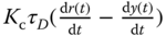 is not practically implementable and the differentiation of the output signal
  leads to amplification of the measurement noise. Thus, there are a few modifications with regard to the derivative terms. Firstly, in order to avoid the problem caused by a step reference trajectory change (the so-called derivative kick problem (Hägglund (2012))), the derivative action is only implemented on the output signal
  . Secondly, in order to avoid amplification of the measurement noise, a derivative filter is in a companionship with the derivative term
  .
.
A commonly used derivative filter is a first order filter and has its time constant linked as a percentage to the actual derivative gain  in the form:

where  is typically chosen to be 0.1 (10%).
  is chosen to be larger if the measurement noise is severe.
With the derivative filter  , a typical PD controller output is calculated as
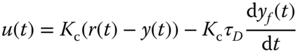
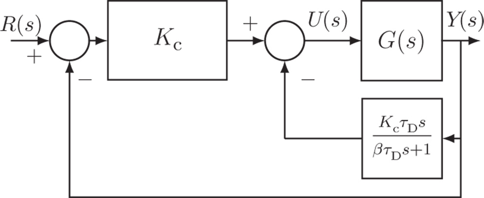
Figure 1.4 PD controller structure in implementation.
where  is the filtered output response using (1.11). In a Laplace transform, the control signal is expressed as

Figure 1.4 shows the block diagram used for implementation of a PD controller with a filter.
If the derivative filter was not considered in the design, there is a certain degree of performance uncertainty due to the introduction of the filter. This may not be ideal for many applications. Designing a PD controller with the filter included will be discussed in Section 3.4.1.
1.2.3 Proportional Plus Integral Controller
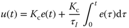
A proportional plus integral (PI) controller is the most widely used controller among PID controllers. With the integral action, the steady-state error that had existed with the proportional controller alone (see Example 1.1) is completely eliminated. The output of the controller  is the sum of two terms, one from the proportional function and the other from the integral action, having the form,
where  is the error signal between the reference signal
  and the output
  ,
,  is the proportional gain, and
  is the integral time constant. The parameter
  is always positive, and its value is inversely proportional to the effect of the integral action taken by the PI controller. A smaller
  will result in a stronger effect of the integral action.
The Laplace transform of the controller output is

with  being the Laplace transform of the error signal
  . With this, the Laplace transfer function of the PI controller is expressed as
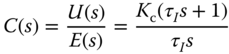
Figure 1.5 shows a block diagram of the PI control system.
The example below is used to illustrate closed-loop control with a PI controller. For comparison purpose, we use the same plant as that used in Example 1.1.
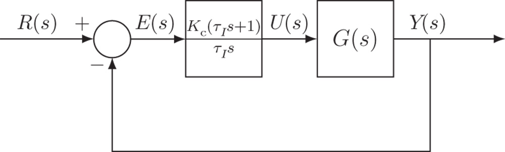
Figure 1.5 PI control system.
It is often the case that the output of a PI control system exhibits overshoot to a step reference signal. The percentage of overshoot increases as higher control performance demanded. This may cause a conflict in the PI control performance specifications: on the one hand a fast control system response is desired, and yet on the other hand, the overshoot is not desirable when step reference changes are performed. The overshooting problem in reference change could be reduced by a small change in the configuration of the PI controller. This small change is to put the proportional control on the output signal  , instead of the feedback error
  . More specifically, the control signal
  is calculated using the following relation,
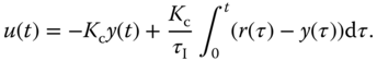

Figure 1.6 Closed-loop step response of a PI control system (Example 1.2).

Figure 1.7 IP controller structure.
Applying a Laplace transform to this equation leads to the Laplace transform of the controller output in relation to the reference and the output as
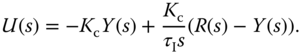
Figure 1.7 shows a block diagram of this PI closed- loop control configuration. This type of implementation is called an IP controller in the literature, which is an alternative PI controller configuration. In Section 2.4, this PI controller structure is examined in the context of a reference filter within the framework of a two degrees of freedom control system. To demonstrate how this simple modification in the PI controller configuration can reduce the overshoot effect, we examine the following example.
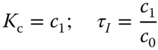
Another form of PI controller, perhaps more convenient for model-based controller design as in Chapter 3, is described by:

This form of PI controller is identical to the original PI controller structure when the parameters of  and
and  are selected as
1.2.4 PID Controllers
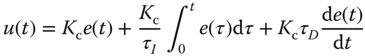
A PID controller consists of three terms: the proportional (P) term, the integral (I) term, and the derivative (D) term. In an ideal form, the output  of a PID controller is the sum of the three terms,
where  is the feedback error signal between the reference signal
  and the output
  , and
, and  is the derivative control gain. The Laplace transfer function of the PID controller is
If the design is sound, the sign of  is positive. If the sign of
  is negative, the derivative control term is to be neglected and instead a PI controller should be chosen.
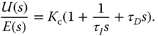
Analogously to the proportional plus derivative controller described in Section 1.2.2, for most of the applications the derivative control is implemented on the output only with a derivative filter. For this reason, the control signal  is expressed in the following form:

Figure 1.9 shows the block diagram of the PID controller structure.
To reduce the overshoot in output response to a step reference change, the proportional term in the PID controller may also be implemented on the plant output. In this case, the control signal is calculated using

Accordingly, the Laplace transform of the control signal is expressed as

Figure 1.10 shows a block diagram of the alternative PID controller structure (called an IPD controller).
The example below is used to illustrate the effect of the derivative term in the closed-loop control. The starting point is the PI controller designed in Example 1.3, based on which a derivative term is introduced.
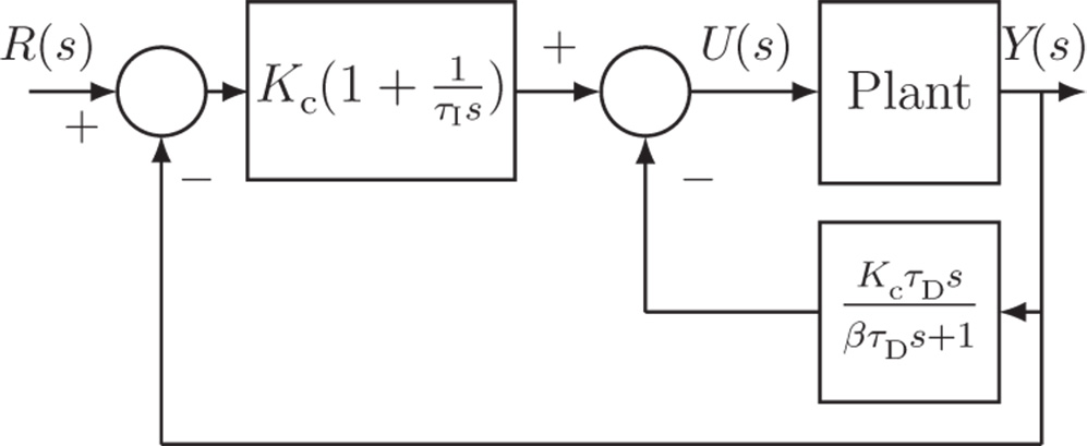
Figure 1.9 PID controller structure.
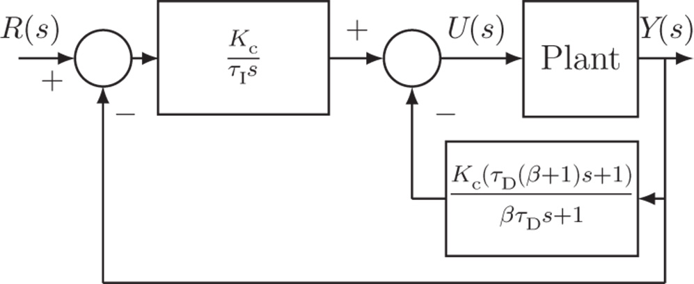
Figure 1.10 IPD controller structure.
1.2.5 The Commercial PID Controller Structure
In the PID controller design, the following structure is commonly used for determining the parameters  ,
,  and
and  , where the controller transfer function
  is expressed as
However, as demonstrated in this section, there are several variations in PID controller structure available for the realization of the control system, and different realization leads to different control system performance with the same set of PID controller parameters.
In order to be more flexible to the users, the commercial PID controllers (see Alfaro and Vilanova (2016)) from manufacturers such as ABB, Siemens, and National Instruments take the following general form with the Laplace transform of the control signal:

where the coefficients  and
and  are for the weighting on the reference signal, and as before, the coefficient
  determines the appropriate derivative filtering action. There are several special combinations of the parameters
  ,
,  , and
, and  that are commonly encountered.
- When
 ,
,  , and
, and  , the PID controller becomes identical to the case shown in Figure 1.9, where the derivative control with filter is implemented on the output only.
 - When
 and
and  , the PID controller becomes the IPD controller shown in Figure 1.10, where both the proportional control and derivative control are implemented on the output only.
 - When
 ,
,  , and
, and  , the implementation of the PID controller puts proportional control, integral control, and derivative control with filter on the feedback error
  .
. - When
 ,
,  , and
, and  , the PID controller becomes the case where no derivative filter is used in the implementation. This will severely amplify the measurement noise.
It is worthwhile emphasizing that the parameters  and
and  only affect the closed-loop response to the reference signal
  and they play no role in the closed-loop stability. We have examined the cases where
  and
and  are either 0 or 1. However, we can extend the results to the situations where the parameters are between 0 and 1 and expect a compromised result. Upon understanding their roles, we can choose the appropriate coefficients according to the actual applications.
1.2.6 Food for Thought
- The PID controllers are expressed in terms of the parameters
 ,
,  and
and  . What are the possible signs of
  ,
,  and
and  ?
? - When you increase the magnitude of
 , do you expect the action of proportional control to decrease or increase? When you increase
  , do you expect the action of integral control to decrease or increase? when you increase
  , do you expect the action of derivative control to decrease or increase?
 - What are the roles of integrator in a PID controller?
- Can you implement the integrating control on output only? If not, explain the reason.
- In many applications, we will put the proportional control on the feedback error, which is the original PI controller. Can you reduce the overshoot by using a ramp reference signal in the early part of the response?
1.3 Classical Tuning Rules for PID Controllers
This section will discuss the classical tuning rules that have existed for the past several decades and have withstood the test of time. Although all tuning rules are rule-based, there is still certain knowledge assumed for the system to be controlled.
1.3.1 Ziegler–Nichols Oscillation Based Tuning Rules
Ziegler–Nichols oscillation based tuning rules are to use closed-loop controlled testing to obtain the critical information needed for determining the PID controller parameters.
In the closed-loop control testing, the controller is set to proportional mode without integrator and derivative action. The sign of  must be the same as the steady-state gain of the plant for the reason of introducing negative feedback in the control system. With the proportional closed-loop control, the feedback gain
  is set to be a very small value in magnitude to begin the experiment. The value of
  is gradually increased until the control signal
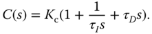
  exhibits sustained oscillation (see Figure 1.12). There are two parameters obtained from this test: the value of
  that has caused the oscillation and the period of the oscillation. We denote this particular
  as
as  and the period as
  . With these two parameters, the PID controller parameters are presented for the Ziegler–Nichols tuning rules in Table 1.1.
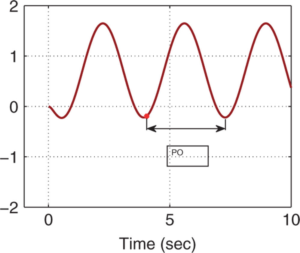
Figure 1.12 Sustained closed-loop oscillation (control signal).
Table 1.1 Ziegler–Nichols tuning rule using oscillation testing data.
 |
 |
 |
||||
| P |  |
|||||
| PI |  |
 |
||||
| PID |  |
 |
 |
A proportional control will not cause sustained oscillation for first order plant and second order plant with a stable zero. Thus, the tuning rule is not applicable to these two classes of stable plants. The following example is used to illustrate an application of the tuning rule.
In general, the Ziegler and Nichols tuning rules using the oscillation method lead to quite aggressive responses with oscillations in closed-loop responses that are undesirable for many control applications. In Tyreus and Luyben (1992), a smaller  and a larger
  are recommended to reduce the oscillations, which have the following values:

It is important to point out that generating sustained oscillation by increasing the controller gain is not a safe operation because a small error in the tuning process could cause the closed-loop system to become unstable. This unsafe procedure is replaced by using relay feedback control in Chapter 9, which also produces a sustained closed-loop oscillation.
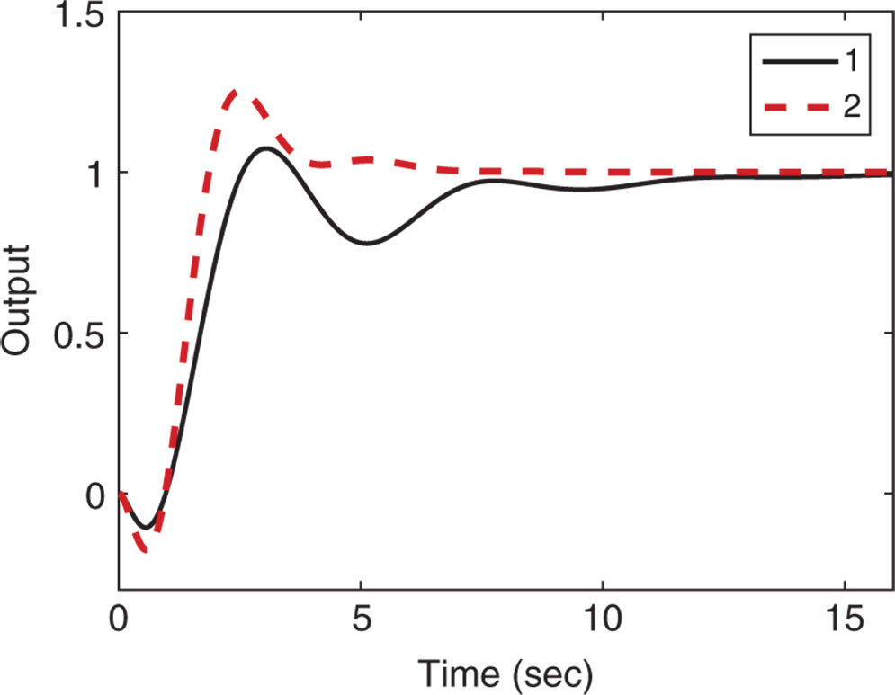
Figure 1.13 Comparison of closed-loop output response using Ziegler–Nichols rules (Example 1.5). Key: line (1) PI control; line (2) PID control.
1.3.2 Tuning Rules based on the First Order Plus Delay Model
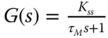
The majority of tuning rules existing in the literature are based on a first order plus delay model, which has the following transfer function:
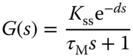
where  is the steady-state gain of the system,
  is the time delay, and
  is the time constant. This is mainly because the primary applications of tuning rules are for process control where typically the process is stable with time delay. There are many methods available for obtaining a first order plus delay model. Among them is an incredibly simple procedure that is called fitting a reaction curve. This reaction curve is the so-called step response test.
The reaction curve is obtained by performing a plant step response test in open-loop operation, therefore we assume that the plant is stable, although it could be applied to integrating plant with caution. When performing this test, the plant input signal  takes a step change from an initial constant value
  to a normal operation value,
  ; the measurement of the plant output signal
  in response to the step input change gives us the plant step response test data or the reaction curve. The response test completes when the value of the output signal reaches a constant or the signal fluctuates around a constant value due to noise and disturbances. Figure 1.14 illustrates a typical set of step response testing data, with the step change occurring at time
  . Figure 1.14(a) shows that the input takes a step change from the initial value
  to the final value
  and Figure 1.14(b) shows the actual output response from the steady-state output position
  to the steady-state output position
  .
.
The plant information obtained from the test includes the steady-state gain, defined as
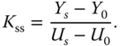
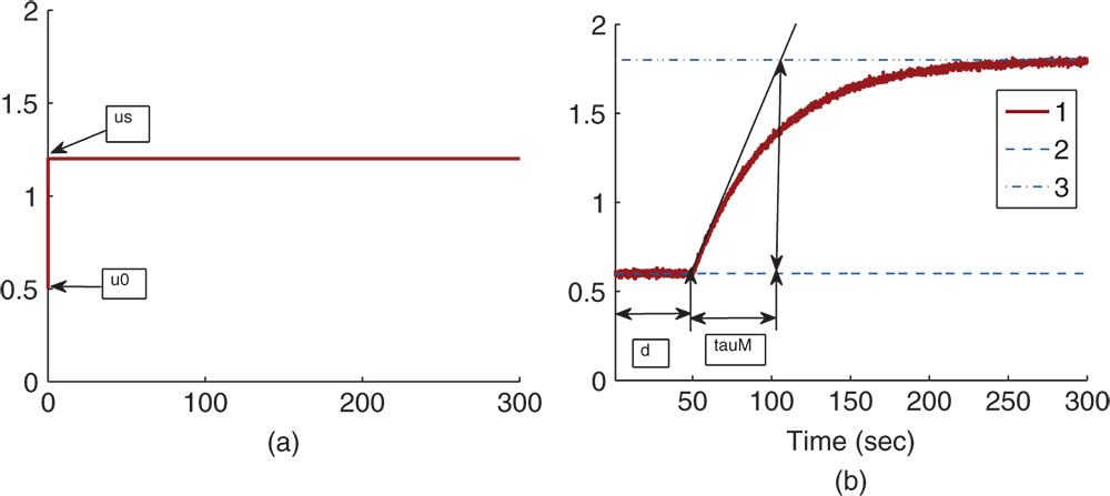
Figure 1.14 Step response data. (a) Input signal. (b) Output signal. Key: line (1) the output response; line (2) steady-state output position before the response ( ); line (3) steady-state output position in completion of the response (
 ).
).
The time delay  is shown in the figure, which is the delayed time when the output responds to the change in the input signal. The parameter time delay
  reflects the situation that the output response remains unchanged despite the step input signal being injected. Thus, it is estimated using the time difference between when the step reference change occurred (
 for this figure) and when the output response moved away from its steady-state value (see the time interval in Figure 1.14(b) marked with the first set of arrows). A line with maximum slope is drawn on Figure 1.14(b), which is intersected with the line corresponding to the indicator of
  . The intersecting point shown in Figure 1.14(b) determines the value of
  that is a measurement of the dynamic response time.
Alternatively, because the step response of a first order system ( ) to a unit step input signal can be expressed as
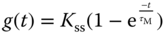
and when the variable time  ,
,

thus, we can determine the time constant  using 63.2% of the rising time in the step response. This estimation of time constant gives a different value from the case when using the maximum slope approach. For the majority of the applications, this will result in a smaller time constant
  , and from the empirical tuning rules stated in the later part of the section, a smaller proportional gain
  will follow. One can evaluate this approach as an exercise using Problem 1.2.
Essentially, the step response test gives the parameters in the first order plus delay description of the process as in (1.44).
There is a second set of Ziegler–Nichols tuning rules that is based on the plant step response test data. This is also called the Ziegler–Nichols tuning rules using reaction curve. With these parameters, Ziegler–Nichols tuning rules using a reaction curve are given in Table 1.2. By the nature of this testing procedure (open-loop testing), the tuning rules should apply to stable systems.
Table 1.2 Ziegler-Nichols tuning rules with a reaction curve.
 |
 |
 |
||||
| P |  |
|||||
| PI |  |
 |
||||
| PID |  |
 |
 |
Table 1.3 Cohen–Coon tuning rules with a reaction curve.
 |
 |
 |
||||
| P | 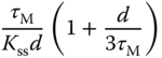 |
|||||
| PI | 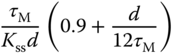 |
 |
||||
| PID | 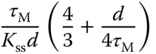 |
 |
 |
There is another set of tuning rules that are derived based on the reaction curve, termed Cohen and Coon tuning rules. Table 1.3 gives the PID controller parameters calculated from Cohen and Coon tuning rules.
For the estimation of time delay  ,
,  , and
, and  when using MATLAB, it is a fairly straight forward procedure to draw the lines and pinpoint the data points. The MATLAB command for finding the point on a graph is called ginput. For example, by typing
[a,b]=ginput(1) a cross hair will appear on the MATLAB figure and a double click on the point of interest will yield the exact values we need. This graphic procedure will be demonstrated in the example section (see Section 1.5).
1.3.3 Food for Thought
- Can you apply Ziegler-Nichols oscillation tuning method to a first order system? Why?
- Can you apply the reaction curve based tuning rules to unstable systems? Why?
- How do we decide the sign of the proportional feedback controller gain when using the Ziegler-Nichols oscillation method?
- Can you envisage any potential danger when using Ziegler- Nichols oscillation method?
- How do you design a step response experiment?
- What information will the step response experiment provide?
- How do you determine steady-state gain, parameter
 and time delay
  from a reaction curve?
 - What are your observations when comparing Ziegler-Nichols and Cohen-Coon tuning rules, in terms of signs and values of
 ,
,  and
and  ?
? - Is there any desired closed-loop performance specification among the tuning rules?
1.4 Model Based PID Controller Tuning Rules
This section will discuss the PID controller tuning rules that are derived based on a first order plus delay model. These tuning rules worked well in applications.
1.4.1 IMC-PID Controller Tuning Rules
The internal model control (IMC)-PID tuning rules (Rivera et al. (1986)) are proposed on the basis of a first order plus delay model:

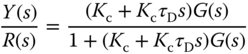
When using the IMC-PID tuning rules, a desired closed-loop response is specified by the transfer function from the reference signal to the output:
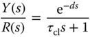
where  is the desired time constant chosen by the user. The PI controller parameters are related to the first order plus delay model and the desired closed-loop time constant
  , which are given as:

If the system has a second order transfer function with time delay in the following form:

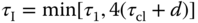
then a PID controller is recommended. Assuming that  , then the PID controller parameters are calculated as
Later on, it was realized that the choice of  basically led to a pole-zero cancellation in the control system. Such a pole-zero cancellation will limit, as discussed in the next chapter, the control system performance in the disturbance rejection, particularly when
  is large4. In Skogestad (2003), the IMC-PID tuning rules are modified to reduce the integral time constant as
while  and
and  are unchanged from (1.47).
The IMC-PID controller tuning rules are also extended to integrating systems in Skogestad (2003). Although the system has an integrator as part of its dynamics, integral control is still required for disturbance rejection (see Chapter 2).
Assuming that the system has the integrator with delay model:
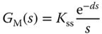
then a PI controller is recommended with the following parameters:
If the transfer function for the integrating system has the form:

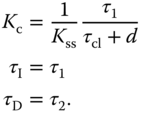
then a PID controller is recommended to have the following parameters:

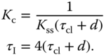
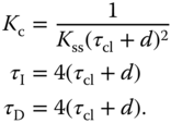
If the system has a double integrator with the transfer function
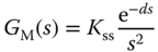
then a PID controller is recommended with the following parameters:
The IMC-PID controller tuning rules will be studied in Examples 2.1 and 2.2.
1.4.2 Padula and Visioli Tuning Rules
Several sets of tuning rules were introduced in Padula and Visioli (2011) and Padula and Visioli (2012). These tuning rules are based on the first order plus delay model:

Table 1.4 Padula and Visioli tuning rules (PI controller).
 |
 |
||
 |
 |
 |
|
 |
 |
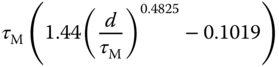 |
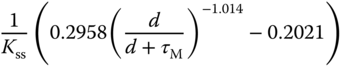
Table 1.5 Padula and Visioli tuning rules (PID controller).
 |
 |
||
 |
 |
 |
|
 |
 |
 |
|
 |
 |
 |
They were derived using optimization methods for minimizing an error function together with the sensitivity peak in the frequency domain (see Chapter 2).
Here, we only include two sets of the tuning rules introduced for disturbance rejection in their paper. Tables 1.4 and 1.5 present the tuning rules for PI and PID controllers, respectively. Each table contains two sets of rules. For the specification of  (
( corresponds to the sensitivity peak (see Chapter 2)), the set of tuning rules is expected to produce a slower closed-loop response in comparison to that with
  . It is worthwhile mentioning from Tables (1.4) and (1.5) that both PI and PID controller parameters are invalid for the time delay
  because as
  , the proportional control gain
  .
.
A frequency response analysis for the Padula and Visioli tuning rules based control system will be presented in Chapter 2 where an example (see Example 2.4) will be given to show the sensitivity functions and their Nyquist diagrams.
1.4.3 Wang and Cluett Tuning Rules
In Wang and Cluett (2000), a first order plus delay model was used to derive several tuning rules for PID controllers. The rules were calculated using a frequency response analysis based on the ratio of the time constant  to the time delay
  , which is defined as
  . A desired closed-loop time constant is chosen as a scale of the time delay
  . Among them, which works quite well in applications, is a particular choice with the desired closed-loop time constant being equal to the time delay
  . For this choice, the PID controller parameters are presented in Table 1.6.
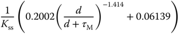
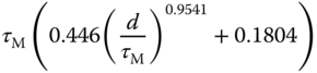
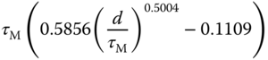
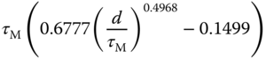
Table 1.6 Wang–Cluett tuning rules with reaction curve ( ).
).
 |
 |
 |
||||
| P |  |
|||||
| PI |  |
 |
||||
| PID |  |
 |
 |
1.4.4 Food for Thought
- In the IMC-PID controller tuning rules, if a faster closed-loop response is desired, would you increase or decrease the desired closed-loop time constant
 ?
? - For the tuning rules derived by Padula and Visioli, are there any closed-loop performance parameters chosen by the user?
- Intuitively, would you increase the proportional controller gain
 if the PID controlled system is unstable when using the Padula and Visioli's tuning rules?
 - Would you increase the integral time constant
 if the PID controlled system is oscillatory when using the Padula and Visioli's tuning rules?
1.5 Examples for Evaluations of the Tuning Rules
Several examples are presented in this section for evaluation of the tuning rules that are based on the first order plus delay model.
1.5.1 Examples for Evaluating the Tuning Rules
The first example is based on a first order plus delay plant and the second example is based a high order plant so that an approximation is made during the graphic procedure.
In reality, instead of a pure first order plus delay dynamics, there are more or less additional dynamics in the system. The tuning rules are applicable for a more complex system. We illustrate how to apply the tuning rules using the example below. This example also illustrates the fact that we need to be cautious when applying the tuning rules and be aware of their limitations.
Table 1.7 PI controller parameters with reaction curve.
 |
 |
|||
| Ziegler–Nichols | 3.1714 | 63 | ||
| Cohen–Coon | 3.3381 | 32.7131 | ||
| Wang–Cluett | 2.0571 | 41.4811 |
Figure 1.16 Closed-loop unit step response with PI controller (Example 1.6). Key: line (1) Ziegler–Nichols tuning rule; line (2) Cohen–Coon tuning rule; line (3) Wang–Cluett tuning rule.
The following example illustrates the applications of the Padula and Visioli tuning rules.
Figure 1.17 Unit step response (Example 1.7).
Table 1.8 PI controller parameters with reaction curve.
 |
 |
|||
| Ziegler–Nichols | 6.4 | 108 | ||
| Cohen–Coon | 6.5667 | 75.9231 | ||
| Wang–Cluett | 3.8867 | 127.2154 |
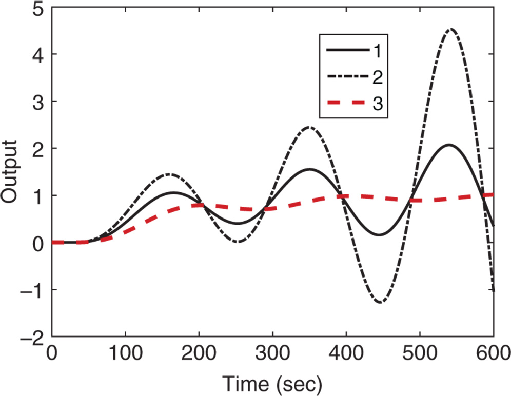
Figure 1.18 Closed-loop unit step response with PI controller (Example 1.7). Key: line (1) Ziegler–Nichols tuning rule; line (2) Cohen–Coon tuning rule; line (3) Wang–Cluett tuning rule.
1.5.2 Fired Heater Control Example
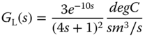
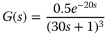
A fired heater using gas fuel is a heating furnace that is typically used for household heating in the winter times. In this case study, the input to the heating furnace is the feed rate of the gas fuel and the output is the heater outlet or the room temperature in a house. Because the temperature sensors are located away from the heating source, there is a time delay in the measured temperature when the input feed rate changes. Additionally, depending on the operating conditions of the input feed rate, the dynamic response of the temperature is different. Two transfer function models are given in Ralhan and Badgwell (2000) to describe the operations of a gas fired heater at a low fuel operation and a high fuel operation. At the low fuel operating condition, the transfer function is described as
and at the high fuel operating condition,
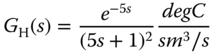
where the time constant is in minutes. Note that there are dramatically differences in time delay and the steady-state gain of the transfer function models.
In this study, we will introduce the effect of input disturbance in the closed-loop simulation by adding a step signal with negative magnitude to the control signal. This input disturbance represents a sudden change in the process that causes the output temperature drop. The effect of this disturbance is further discussed in Chapter 2.
1.6 Summary
This chapter has introduced the basics in PID control systems. It is important for us to understand the roles of proportional control, integral control and derivative control. The simple modification with the implementation of PID controller by putting the proportional control on output only reduces the overshoot in the step reference response. For some applications, avoiding the overshoot is important because the requirement is associated with the system's operational constraints while for other applications the overshoot is preferred if the PID controller is used in an inner-loop system (see Chapter 7). Additionally the derivative control should be implemented with a derivative filter to avoid amplification of measurement noise and the derivative control should be implemented on the output only to avoid the scenario of derivative ‘kick’.
Several sets of tuning rules have been introduced in this chapter. These tuning rules are very simple and easy to use if the system can be approximated by a first-order-plus delay model. However, they offer no guarantees on the closed-loop performance as demonstrated by the simulation examples. Some of the examples used in this chapter will be analyzed using the Nyquist stability criterion and sensitivity functions in Chapter 2.
1.7 Further Reading
- Text books in control engineering include, Franklin et al. (1998), Franklin et al. (1991), Ogata (2002), Golnaraghi and Kuo (2010), Goodwin et al. (2000) and Astrom and Murray (2008).
- Process control books include Marlin (1995), Ogunnaike and Ray (1994), Seborg et al. (2010).
- There are many books published on PID control, including Astrom and Hagglund (1995), Astrom and Hagglund (2006), Yu (2006), Johnson and Moradi (2005), Visioli (2006), Tan et al. (2012). PID control of multivariable systems is discussed in Wang et al. (2008).
- Tuning rules are compiled as a book (O'Dwyer (2009)). PID controller tuning rules with performance specifications derived from frequency response analysis are introduced in Wang and Cluett (2000).
- The survey and tutorial papers on PID control include Åström and Hägglund (2001), Ang et al. (2005), Li et al. (2006), Knospe (2006), Cominos and Munro (2002) and Visioli (2012), Blevins (2012).
- A web-based laboratory for teaching PID control is introduced in Ko et al. (2001), Yeung and Huang (2003).
- The issues associated with derivative filters in PID controller are addressed in Luyben (2001), Hägglund (2012), Hägglund (2013), Isaksson and Graebe (2002), Larsson and Hägglund (2011).
- Improving reference tracking and reducing overshoot is discussed for an existing controller in an industrial environment (Visioli and Piazzi (2003)).
- Ziegler-Nichols tuning formula is refined in Hang et al. (1991) and for unstable systems with time delay in De Paor and O'Malley (1989). The ZieglerNichols step response method is revisited from the point of view of robust loop shaping (Åström and Hägglund (2004)). There is a set of tuning rules for integrating plus delay model in Tyreus and Luyben (1992), which was extended to PID controllers in Luyben (1996).
Problems
- 1.1 The following system is given to practice the Ziegler-Nichols tuning rules based on oscillation testing data to determine the PID controller parameters:

- Build a Simulink simulator using closed-loop proportional control with a controller
 for the system. The sampling interval
  is chosen to be 0.1 sec.
 - Find the PI and PID controller parameters using Table 1.1.
- Implement the PI and PID controllers in Simulink with a step reference signal by putting both proportional and derivative control on the output only.
- What are your observations with respect to the closed-loop performance of the PI and PID control system?
- Build a Simulink simulator using closed-loop proportional control with a controller
- 1.2 In the majority of the tuning rules, the key step is to find a first order plus delay approximate model for step response testing data. Because the step response of a first order system (
 ) to a unit step input signal can be expressed as

we can determine the time constant
 using 63.2 percent of the rising time in the step response.
- Why does the 6.32 percent of the rising time correspond to the time constant
 ?
? - Construct a graphic method to find a first order plus time delay model for the following system:
- Compare this first order plus delay model with that found in Example 1.7.
- Find the PID controller parameters using Table 1.2 and compare the closed-loop simulation results with the ones given in Example 1.7. What are your observations?
- If the step response data contained severe measurement noise, would it be more difficult to determine the rising time?
- Why does the 6.32 percent of the rising time correspond to the time constant
- 1.3 The transfer function for the fired heater system with high operating condition introduced in Section 1.5.2 is given as
- Find the first order plus delay approximate model for this transfer function using the graphic method in Section 1.3.2. The sampling interval
 is chosen to be 1.
 - Determine the PID controllers using Tables 1.2–1.6.
- Evaluate their closed-loop performance by simulating their closed-loop unit step responses. What are your observations in terms of closed-loop performance with respect to the tuning rules?
- Find the first order plus delay approximate model for this transfer function using the graphic method in Section 1.3.2. The sampling interval
- 1.4 The transfer function for the fired heater system with low operating condition introduced in Section 1.5.2 is given as
- Design three PID controllers for this system using IMC-PID controller design equations shown in (1.47) where the desired closed-loop time constant
 , 30 and 40 respectively.
 - Evaluate the closed-loop control system performance for the three PID controllers by simulating the closed-loop unit step response with sampling interval
 sec.
sec. - What are your observations of the closed-loop performance when the desired closed-loop time constant
 increases?
- Design three PID controllers for this system using IMC-PID controller design equations shown in (1.47) where the desired closed-loop time constant
- 1.5 The two transfer functions obtained from the fired heater system are drastically different at the two operating conditions (see (1.61)–(1.62)). Hence, the PID controllers are different for the two operating conditions. Assume that we would only use one PID controller for both operating conditions.
- Design IMC-PID controller (
 ) for the fired heater system at high operating condition using
  with
with  .
. - Evaluate the closed-loop performance by simulating the two PID control systems: (1)
 and
and  ; (2)
; (2)  and
and  , respectively.
 - Let
 denote the PID controller found from Problem 1.4 with
  . Evaluate the closed-loop performance by simulating the two PID control systems: (1)
  and
and  ; (2)
; (2)  and
and  .
. - Based on the simulation studies, which controller should we recommend?
- Increase the desired time constant
 to 40 and repeat the evaluations. What would be the recommendations for the choice of
  ?
?
- Design IMC-PID controller (

 and calculating the value of the transfer function.