9
Automatic Tuning of PID Controllers

9.1 Introduction

Relay feedback control has been one of the key instruments used in the automatic tuning of PID controllers. Its application is associated with the identification of process frequency response information via the self-generated excitation signals in a closed-loop operation. Because it is in a closed-loop operation, the feedback control effect maintains the system around its operating condition while conducting the experiment.

This chapter will discuss the automatic tuning of PID controllers where the process frequency response information is obtained from relay feedback experiments and the PID controllers are designed using the design methods introduced in Chapter 8.

9.2 Relay Feedback Control

This section will discuss relay feedback control systems in combination with hysteresis or with an integrator. Simulink tutorials are presented for both cases, which is convenient for simulation studies and experimental validations.

9.2.1 Relay Control with Hysteresis

In applications, because of measurement noise, a hysteresis element is incorporated within the relay feedback control mechanism to avoid possible random switches due to the effect of noise. Figure 9.1 illustrates a block diagram of relay feedback control.

For the purpose of relay feedback control, there are a few parameters that need to be defined.

1. A plant steady-state operating condition with input signal and output signal is chosen based on which relay control experiment will be carried out. For some applications, the steady-state input and output signals are zero.
2. The amplitude of the relay control signal is chosen as parameter , which represents the variations of the input signal at the steady-state operating condition.
3. The hysteresis parameter is chosen to be , which is used to prevent the triggering of relay switching from random noise. If the standard deviation of the measurement noise is , then approximately the hysteresis parameter is chosen to be .

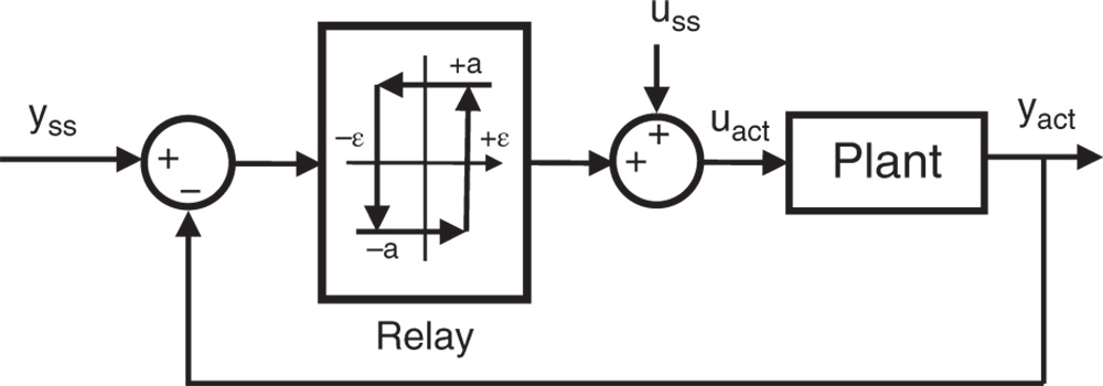
Figure 9.1 Block diagram of relay feedback control.

We define the deviation variable of the control signal as

and the initial condition of the deviation control signal as . We assume that the system is already operating at the steady state. With the actual measurement of the output at the sampling time , the closed-loop control signal is calculated using the following relay switching rules:

(9.1)

and

(9.2)

where 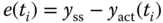is the feedback error at the sampling time .

It is worthwhile emphasizing that the relay switching rule given in (9.1) is for the systems that have a positive steady-state gain. For the systems having a negative steady-state gain, the deviation variable is calculated as

(9.3)

(9.4)

Clearly, the relay feedback control is a nonlinear control law with a small amount of a priori information required and it is very easy to implement.

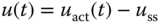
It is known (Astrom and Hagglund (1984), Astrom and Hagglund (1988)) that this relay controlled system will generate a sustained periodic oscillation that contains the fundamental frequency at the point of the Nyquist curve of the process, which approximately has the imaginary part as , as shown in Figure 9.2. One immediately pays attention to the location of the frequency on the Nyquist curve. If the hysteresis value is chosen to be zero, then the frequency becomes the cross-over frequency on the Nyquist curve if a proportional controller is used. This was indeed the key link between the classical Ziegler–Nichols tuning rules and the first generation of auto-tuners (Astrom and Hagglund (1984), Astrom and Hagglund (1988)). The second point is that if the hysteresis is increased, while maintaining the same amplitude , the frequency is reduced, meaning that the oscillation period is increased.

Under relay feedback control, there are several classes of systems that will have a sustained periodic oscillation. In general, these systems should be stable to ensure safety of the operation during experiments. They include the first order plus delay systems, systems with higher order dynamics, systems with non-minimum phase behavior and higher order under-damped systems. The common feature of these systems is that their Nyquist curve will expand to the second and third quadratures on the complex plane, as shown in Figure 9.2. For a first order system, relay feedback control will not generate sustained periodic oscillation unless there are additional dynamics from actuation and measurement involved leading to a higher order system as a result.

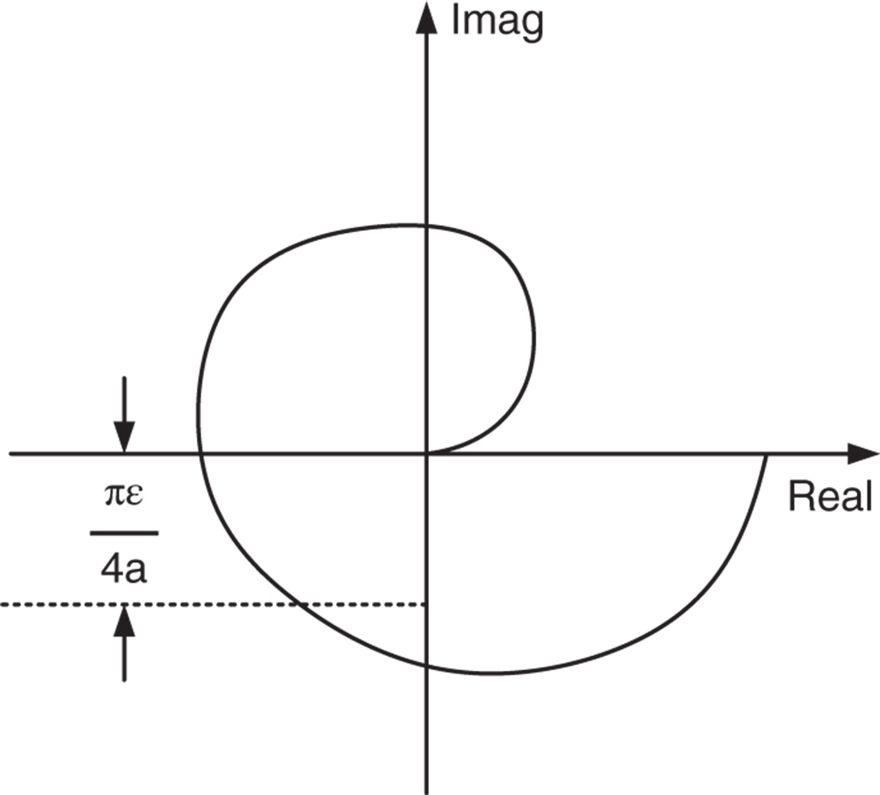
Figure 9.2 Location of on a Nyquist curve.

The following tutorial is written to produce a MATLAB function that can be used for Simulink simulations and for real-time implementations.

---

Tutorial 9.1

This tutorial is to illustrate how to implement the relay feedback control algorithm in real time. The core of this activity is to produce a MATLAB embedded function that can be used in a Simulink simulation as well as in xPC Target implementation. The entire embedded MATLAB function completes one cycle of computation for the relay feedback control signal. For every sampling period, it will repeat the same computation procedure.

Step by Step

1. Create a new Simulink file called RelayH.slx
2. In Simulink's directory of User-Defined Functions, find the icon of embedded MATLAB function and copy it to the RelayH model.
3. Click on the icon of the embedded function, and define the input and output variables to the RelayH model so that the embedded function has the following form:

   function uCurrent=RelayH(e,Ra,epsilon) 

   where uCurrent is the calculated relay control signal at the sampling time , the first element(e) is the feedback error, the second element (Ra) is the relay amplitude, and epsilon is the hysteresis used to avoid random switches caused by noise.

4. At the top of the embedded function, find Model Explorer among the Tools. When opening the Model Explorer, select discrete for the update method and input Deltat into the sample time; select Support variable-size arrays; select Saturate on integer overflow; select Fixed point. Click Apply to save the changes.
5. We need to edit the input and output data ports in order to let the embedded function know which input ports are the real time variables and which are the parameters. This editing task is performed using Model Explorer.
   • click on e, on Scope, select input, assign port 1 and size -1, complexity Inherited, type Inherit: Same as Simulink.
   • The remaining two inputs to the embedded function are the parameters required in the computation. Click on Ra, on Scope, select Parameter and click Tunable and click Apply to save the changes. Repeat the same editing procedure for the epsilon.
   • To edit the output port from the embedded function, click on uCurrent, on Scope, select Output, Port 1, Size -1, Sampling Model Sample based, Type Inherit: Same as Simulink, and click on Apply to save the changes.
6. In the following, the program will declare those variables that are stored in the embedded function during each iteration for their dimensions and initial values. uPast is the past control signal . Enter the following program into the file:

   persistent uPast
   if isempty(uPast)
     uPast=Ra;
   end 

7. Check to see if the feedback error is within the specified hysteresis level () and if so, the control signal remains unchanged. Otherwise, the relay control signal equals to the sign of the feedback error multiplying the amplitude of the relay, followed by updating the past control signal . Continue entering the following codes into the program.

   if abs(e)<=epsilon
     uCurrent=uPast;
   else
     uCurrent=sign(e)*Ra;
     uPast=uCurrent;
    end 

8. Test this program using Simulink simulator you build for Example 9.1.

---

---

Example 9.1

Use relay feedback control to generate sustained oscillation for the following system:

(9.5)

where the measurement noise is a band-limited white noise with noise power 1 and sampling interval and a gain . In the closed-loop relay feedback control, the relay amplitude is chosen to be , , and the sampling interval .

Solution. Choosing the relay amplitude , we build the Simulink simulator as shown in Figure 9.3 where the band limited white noise is used with a gain 0.1 to simulate the measurement noise. We also used the RelayH.slx function in the closed-loop simulation as the relay feedback controller. Note that the noise is added in the closed-loop system, which will affect the switching frequency if the parameter is too small.

Figure 9.3 Simulink diagram for the relay feedback control.

Figure 9.4 Relay feedback control signals with hysteresis (Example 9.1). (a) . (b) .

We first use a small hysteresis value , and the relay feedback control signals are shown in Figure 9.4(a). It is seen that, because of the noise, it takes a long time to establish a stable oscillation, and additionally, the control signal responds to the noise, generating fast and random switches. In contrast, when we increase the hysteresis value to , as shown in Figure 9.4(b), the stable oscillation is established rather quickly and the control signal seldom has the fast and random switches triggered by noise once the sustained oscillation is reached.

---

9.2.2 Relay Control with Integrator

Assuming that the plant is stable with all poles on the left half of the complex plane, the relay feedback controller incorporates an integrator in the closed-loop system, as illustrated in Figure 9.5. It is known (Astrom and Hagglund (1984), Astrom and Hagglund (1988)) that this relay controlled system will generate a sustained periodic oscillation that contains the fundamental frequency at the point where the Nyquist curve of the process intersects the imaginary axis as shown in Figure 9.6.

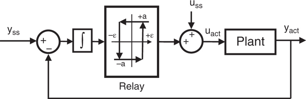
Figure 9.5 Block diagram of integrated relay feedback control.

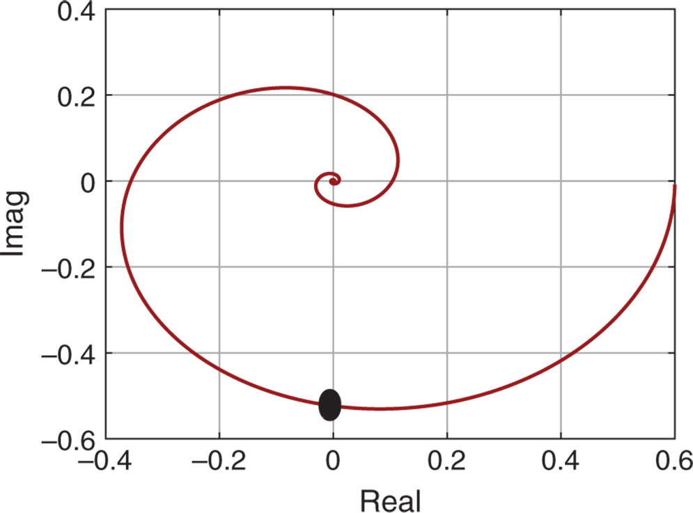
Figure 9.6 Location of on a Nyquist curve when using an integrator with relay.

With the integrator incorporated in the relay feedback control, the frequency is smaller than the case without the integrator, meaning that the oscillation period is larger. The main purpose of choosing this configuration instead of the basic relay feedback control is to ensure that the plant information obtained is contained at the lower and medium frequency range, as illustrated in Figure 9.6. Additionally, because of the integrator, the effect of high frequency measurement noise is minimized, and the need to use a hysteresis for the noise is reduced. It will be shown in Section 9.6 that the proposed configuration is essential in providing the key information of steady-state gain and dominant time constant in the auto-tuner design.

The relay feedback control with integrator is easy to implement. We assume that the system is operating at the steady state with given values of and . The integral error is defined as

With the first order approximation of the derivative , we obtain at the sampling time ,

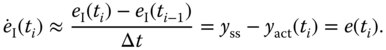
Thus, the integral error is calculated recursively with

The control law for the relay with integrator is summarized as follows. Here, we assume that the steady-state gain of the system is positive.

(9.6)

(9.7)

(9.8)

The following Tutorial is to present a Simulink function for the relay with integrator control law. It is very similar to Tutorial 9.1. With these real time functions, one can convert them into C-code for the real time implementation of the relay feedback control systems.

---

Tutorial 9.2

We assume that one has already written the RelayH.slx codes.

Step by Step

1. Save the RelayH.slx as RelayI.slx
2. The embedded function for the relay with integrator has the following form:

   function uCurrent=RelayI(e,Ra,Deltat) 

   where uCurrent is the calculated relay control signal at the sampling time , the first element(e) is the feedback error, and the second element (Ra) is the relay amplitude, and epsilon is the hysteresis used to avoid random switches caused by noise and Deltat is the sampling interval. As before, we will edit the input and output ports. The new parameter is Deltat, which will be added as a parameter in the editing process.

3. In the following steps, the program will declare those variables that are stored in the embedded function during each iteration for their dimensions and initial values. ‘uPast’ is the past control signal (), and 'eIPast' is the past integrated error signal (). Enter the following program into the file:

   persistent uPast
   if isempty(uPast)
     uPast=Ra;
   end
   persistent eIPast
   if isempty(eIPast)
     eIPast=0;
   end 

4. Calculate the integrated error. Enter the following program into the file:

   eI=eIPast+e*Deltat;
   eIPast=eI; 

5. Check to see if the integrated feedback error is within the specified hysteresis level () and if so, the control signal remains unchanged. Otherwise, the relay control signal equals to the sign of the integrated feedback error multiplying the amplitude of the relay, followed by updating the past control signal . Here, we set the default value of . Continue entering the following codes into the program.

   if abs(eI)<=0.001
     uCurrent=uPast;
   else
     uCurrent=sign(eI)*Ra;
     uPast=uCurrent;
    end 

6. Test this program using Simulink simulator built for Example 9.2.

---

---

Example 9.2

Use of a relay with an integrator controller to generate a sustained oscillation for the following transfer function:

The sampling interval is selected as , and the amplitude of the relay control is . In the closed-loop control simulation, a band-limited white noise with power and sampling interval is used as shown in Figure 9.7(a). Compare the relay feedback closed-loop responses with and without the integrator.

Figure 9.7 Relay feedback control signals with and without integrator (Example 9.2). (a) Noise used in simulation. (b) Relay with integrator. (c) Relay with hysteresis (). (d) Relay with hysteresis ().

Solution. We use the same Simulink configuration as illustrated in Figure 9.3, except replacing the RelayH function by the RelayI function when deploying the relay with integrator controller. Figure 9.7(b) shows the input and output signal for the relay with integrator control system. It is seen that although there is much noise in the system, with hysteresis value almost zero (), the input signal does not respond to the measurement noise.

From Figure 9.7(a) it is seen that the noise amplitude is about 2. Thus, without integrator in the relay control, we choose the hysteresis . Figure 9.7(c) shows the closed-loop responses. With , the relay control does not respond to the measurement noise. However, if the parameter is reduced to 1, then the relay control signal is severely affected by the noise, as seen in Figure 9.7(d). Clearly, is too small for the noise in the system.

From this example, it is seen that by incorporating a hysteresis element with the correct into the relay feedback control, or using the relay with integrator, the correlation of noises between the control input signal and the output signal existing in a general feedback control system is broken, rendering the control input signal noise free in a closed-loop operation. Consequently, system identification under relay feedback control becomes a much simpler task without the noise correlations and complex issues such as identifiability in a closed-loop operation are avoided (Soderstrom et al. (2013), Soderstrom (2018)).

---

9.2.3 Food for Thought

1. How do you determine the noise level in the system in order to choose the hysteresis level ?
2. If the noise is severe and you are not sure about the noise level, would you try to use the relay with integrator approach?
3. If the system is first order, relay feedback control will not generate sustained oscillation. Would you consider to incorporate a delay element to the relay feedback control in order to generate a sustained oscillation? How will you define the input and output data in this situation?
4. Instead of using an integrator, will you be able to use a stable transfer function to achieve the same effect? In comparison, what is the key advantage of using an integrator?
5. Is it possible to use relay feedback control to stabilize an unstable system?

9.3 Estimation of Frequency Response using the Fast Fourier Transform (FFT)

It is well known that under a stable relay feedback control, both control input and process output signals are periodic in nature (Astrom and Hagglund (1984), Astrom and Hagglund (1988), Astrom and Hagglund (1995), Astrom and Hagglund (2006), Hagglund and Astrom (1985)). If a single relay experiment is conducted, a standard Fourier analysis (Kreyszig (2006)) shows that the periodic signals contain the frequencies in multiples of the fundamental frequency as , , , , , where is an odd number. Because of this, many approaches have been proposed to extract meaningful process information from the set of relay feedback control data, including the describing function analysis (Atherton (1975), Astrom and Hagglund (1984)) and fast Fourier analysis (Wang et al. (2001)).

9.3.1 FFT Estimation

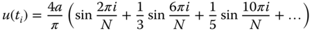
For a period , the Fourier series expansion of the periodic input signal , is expressed as (see Kreyszig (2006)),

(9.9)

Here, we emphasize that the continuous time fundamental frequency is . From (9.9), it is seen that the construction of the periodic signal using the sinusoidal components is predominantly dependent on the first few terms because their contributions decay as the frequency increases.

By choosing sampling interval , the discretized input signal at sampling instant becomes

(9.10)

where is the number of samples within one period. The expression of the discrete time signal reveals the discrete time fundamental frequency as when we compare (9.10) with (9.9). Therefore, the relationship between the continuous time and discrete time frequencies exists as,

(9.11)

The simplest way to estimate the frequency response of the system under relay feedback is to use the FFT. Assuming that the data length is , the Fourier transform of an input signal , , is

(9.12)

and the corresponding Fourier transform of the output is

(9.13)

where . With the computation of the Fourier transformation of both input and output signals, the estimation of the frequency response of the plant is simply (Ljung (1999))

(9.14)

From both (9.12) and (9.13), with the definition of the Fourier transform, it is seen that the corresponding discrete frequency is defined from 0 to with an incremental of , where is the data length.

The remaining tasks are to find which index corresponds to the fundamental frequency in discrete time, followed by converting the discrete time frequency to the continuous time frequency .

An intuitive way to find the fundamental frequency is to find the averaged number of samples of the input signal within one period [see Figures 9.7(b)–(c)]. However, this could potentially lead to an inaccurate result because of the possible random switches in the input signal due to the measurement noise [see Figure 9.7(d)].

Since the input signal exhibits the feature of a periodic signal, the amplitude of the discrete time Fourier transform of the input signal will yield a maximum value at the fundamental frequency . Thus, we will use the maximum value of the amplitude of the Fourier transform as the signature to identify the discrete time fundamental frequency while taking into account of the incremental frequency in a general Fourier transformation.

9.3.2 MATLAB Tutorial using the FFT for Estimation

The following MATLAB tutorial shows how to estimate , , and through Fourier analysis.

---

Tutorial 9.3

In this tutorial, we will estimate the plant frequency response at , , and 0.

Step by Step

1. Create a new file called FFTRelay.m for the MATLAB function.
2. Define the input and output variables for the MATLAB function. Enter the following program into the file:

   function [G1,G3,G5,G0]=FFTRelay(u,y,Deltat) 

   where and are the input and output data from the relay feedback control. Deltat is the sampling interval.

3. Remove the steady-state values of the input and output data to obtain zero mean data. Enter the following program into the file:

   L=length(u);
   u=u-mean(u);
   y=y-mean(y); 

4. Calculate Fourier transform of the input and output signal. Enter the following program into the file:

   Ujw=fft(u);
   Yjw=fft(y); 

5. Estimate the frequency response of the plant for all frequencies. Enter the following program into the file:

   fftEst=Yjw./Ujw; 

6. We find the index that corresponds to the maximum value of the amplitude of the Fourier transform of the input signal, pointing to the fundamental frequency and the estimated plant frequency response . Enter the following program into the file:

   [n1,m1]=max(abs(Ujw));
   P1=m1;
   w1=2*pi*(P1-1)/(L*Deltat);
   G1=fftEst(P1); 

7. We will find the second peak in the amplitude of the Fourier transform of the input signal, pointing to the frequency ω₃. Because of the noise, in many cases, . Enter the following program into the file:

    [n2,m2]=max(abs(Ujw(P1+3:P1+2*m1+3)));
    P3=P1+2+m2;
    w3=2*pi*(P3-1)/(L*Deltat);
    G3=fftEst(P3); 

8. We will locate the third peak in the amplitude of the Fourier transform of the input signal, pointing to the frequency . Enter the following program into the file:

    [n3,m3]=max(abs(Ujw(P3+3:P3+3+2*m1)));
    P5=P3+2+m3;
    G5=fftEst(P5);
    w5=2*pi*(P5-1)/(L*Deltat); 

9. We can also estimate the steady-state gain. Enter the following program into the file:

   G0=fftEst(1); 

10. The estimated frequency responses are exported together with their corresponding frequencies in the following format. Enter the following program into the file:

     G1=[G1 w1];
     G3=[G3 w3];
     G5=[G5 w5];
     G0=[G0 0]; 

11. We can test this program in the Examples 9.3 and 9.4 presented in the next section.

---

9.3.3 Monte-Carlo Simulation Studies

In the Monte-Carlo simulation, the measurement noise is generated with a random initial seed that changes with each simulation to reflect the randomness of the noise and its effect on the estimation results. It means that the measurement noise sequence is unique for each simulation and different from others. Consequently, the estimated parameters for each simulation are unique due to the noise. From the total number of simulations, the mean and variance of the estimated parameters are assessed. This assessment can be performed graphically by plotting the estimated parameters for each run against the original parameters or by calculating the mean and variance of the parameters from the total number of simulations. We choose to use a graphic display of the Monte-Carlo simulation results.

Two examples are presented in this section to show the estimation of frequency response of the system using the FFT with relay feedback control data in a noisy environment. The first case is to investigate the estimation when a relay is used with hysteresis to control the system and the second case is to show the estimation when a relay with an integrator is used to control the system.

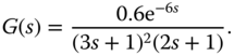
The system under study has the transfer function

The noise used in the simulation is band limited noise with sampling interval (s) and power strength 1 together with a gain 0.1. The simulation time is 800 s. The initial seed used to generate the noise sequence varies from 0 to 68 to form the Monte-Carlo simulation studies. In total, we will conduct 69 simulation studies for the estimation.

---

Example 9.3

The Simulink simulator is set up using the diagram illustrated in Figure 9.3. In the simulation studies, the hysteresis level is chosen to be in order to prevent the relay from random switching triggered by the noise. The relay amplitude is chosen to be . This combination will give the value (see Figure 9.2), which will result in sustained oscillation for this system. Because the measurement noise is used in the closed-loop relay feedback control, it affects the switching pattern of the input signal when the relay element is triggered occasionally by random noise. Figure 9.8(a) shows a section of the input and output data generated using seed for the band limited noise, and Figure 9.8(b) shows the Fourier transform of the input data. The first 1000 data points were removed from the estimation. Using the program FFTRelay.m, the estimation is performed for the sets of data generated from the relay feedback control. Figure 9.8(c) shows the estimated frequency points in clusters for , and from the estimations. From this figure, it is seen that the estimation for is reliable because all estimates are close to the true frequency response at . For the estimation of , there is one failure out of the experiments, which is quite good. For the estimation of , there are a few more failed estimations. The estimation for the steady-state gain is not reliable, as shown in Figure 9.8(d).

Figure 9.8 Frequency response estimation using FFT (Example 9.3). (a) Input and output data using seed . (b) Fourier transform of the input data. (c) Estimated frequency responses ( (o), ω₃ (*), ω₅ ()). (d) Estimated steady-state gain.

It is worthwhile emphasizing that the selection of hysteresis level in relation to amplitude of the relay in a noisy environment is an important task. Without a priori knowledge about the noise level and the gain of the system, their combination is to be revealed often through trial and error experiments.

---

---

Example 9.4

For the relay with integrator control studies, the Simulink simulator is set up using the diagram illustrated in Figure 9.3 with the MATLAB embedded function RelayI.slx produced in Tutorial 9.2.

For the relay with integrator control, the relay amplitude is selected to be one and a very small hysteresis level is used to avoid the possible numerical problem during the relay feedback control. With the exactly same noise sequences used in Example 9.3, the closed-loop relay feedback control system is simulated for different noise sequences. Sustained oscillations are generated for all the experiments. Figure 9.9(a) shows the first segment of the input and output data generated using seed 68 and Figure 9.9(b) shows the Fourier transform of the input data. Figure 9.9(c) presents the estimated results for , and . From this figure, it is seen that the estimated is very good, which is centered at the true frequency response with a small cluster (i.e. a small variance). There is one failure for the estimation of with a larger cluster, also a larger cluster for . There is no reliable estimation for the steady-state gain, as shown in Figure 9.9(d).

It is not essential to use hysteresis in the relay with integrator feedback control because the integral action acting as a low-pass filter has prevented the possible random switches caused by the noise. In comparison, the relay with integrator control is much more robust in the presence of noise, as demonstrated in this example. If the system has severe noises, relay with integrator gives a viable solution to generate a sustained oscillation without having to choose a hysteresis level.

---

9.3.4 Food for Thought

1. Is it correct to say that the periodicity of the input and output signals with relay feedback control plays the key role at obtaining accurate estimated frequency response parameters?
2. Will you still get estimated frequency parameters if the estimated period is wrong?
3. Why do we use the peak amplitude of the Fourier transform of input signal to identify the period of the oscillation?
4. Why can not we reliably estimate the steady-state gain of the system from the periodic input and output data generated by the relay control?
5. If the input and output data are not zero mean, will you be able to correctly obtain the frequency response estimation using the Fourier analysis?

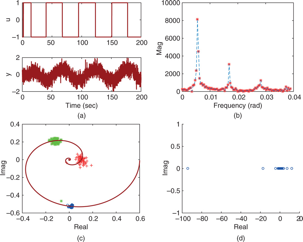
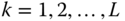
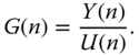
Figure 9.9 Frequency response estimation using FFT (Example 9.4). (a) Input and output data using seed . (b) Fourier transform of the input data. (c) Estimated frequency responses (, , ). (d) Estimated steady-state gain.

9.4 Estimation of Frequency Response Using the frequency sampling filter (FSF)

This section introduces a model based approach for the estimation of process frequency response based on the input and output data collected from relay feedback control. The model is called the FSF model (Bitmead and Anderson (1981),Wang and Cluett (2000)). The advantages of using such a model based approach in comparison with the FFT analysis include that the computation can be performed recursively in real time and the estimated frequency responses have better accuracy because of the model optimization.

9.4.1 Frequency Sampling Filter Model

Assuming that a relay experiment is performed, a set of input and output signals and is obtained. Because the input and output signals are periodic signals, the period in number of samples, denoted by , is calculated and the fundamental discrete frequency is denoted by , where . Also, the backward shift operator is defined as where is a discrete time signal.

Then, associated with the plant frequency response, and , where , the output is expressed using the frequency sampling filter model in the relationship to the input signal as (Bitmead and Anderson (1981),Wang and Cluett (2000)),

(9.15)

where is the FSF output for the zero frequency, defined as

and is the th FSF filter output defined as

and is the output measurement noise assumed to be Gaussian distributed with zero mean and variance . If the input signal is a perfect period signal with period , then, from Fourier analysis (Kreyszig (2006)), it only contains the odd number of frequencies and the magnitude decays as the number increases (see (9.10)). As a result, the outputs from the frequency sampling filters with even numbers are zero in response to the relay feedback control signal , and they could be removed from the sum in (9.15). Figure 9.10 shows a block diagram of the frequency sampling filter model with a reduced number of filters. In practice, because of nonlinearities and other imperfect conditions, the relay control signals may not be perfectly periodic signals. The outputs of the zero frequency sampling filter and the even number of frequency filters may have signals with small magnitudes. To avoid bias errors in estimation, the expression of the output signal will take into consideration the effect of the near zero terms, which yields,

(9.16)

The model in (9.16) with seven complex parameters proves to be adequate for the majority of the applications even in the situation when the relay control does not produce perfect periodic signals.

Figure 9.10 Block diagram of the frequency sampling filter model with reduced order.

With the description of the output signal in terms of the frequency parameters, the next step is to estimate these parameters using the relay feedback control data. Define the complex parameter vector to be estimated as

and its corresponding regressor vector as

where denotes the complex conjugate transpose of .

Assuming that the number of data samples is , then the least squares estimation of has the following analytical solution (Soderstrom and Stoica (1989), Ljung (1999), Soderstrom (2018), Young (2012), Goodwin and Sin (1984)):

(9.17)

For real-time computation, we can use a recursive least squares algorithm to compute the frequency parameter vector at sampling instant (see Goodwin and Sin (1984),Young (2012),Ljung (1999)). Here, a standard recursive least squares algorithm is written in the following steps, where the initial conditions of and are selected by the user or they can also be calculated using the relay testing data based on the least squares algorithm (Wang and Cluett (2000)). The following computation steps are repeated in real time, beginning with the sampling instant .

1. Calculate the estimated parameter vector
   (9.18)
2. Update the covariance matrix using
   (9.19)
   where contains the estimated frequency response parameters at the sampling instant .
3. Go back to step one as the next sampling period arrives.

There are two comments given below.

1. It is worthwhile emphasizing that the estimated zero frequency and even frequency parameters are not reliable due to the near zero magnitudes of their filter outputs due to the periodicity of the input signal. This is illustrated by the Monte-Carlo simulation in the examples.
2. It is important to note that in an ideal situation, the parameter can be determined from the averaged period of the relay control signal. However, this calculation is no longer correct when the relay feedback control does not produce perfectly periodic oscillations. An effective way to calculate is to find the first maximum magnitude of the Fourier transformation of the input signal and the corresponding frequency from which is rounded to the nearest integer to yield the parameter .

9.4.2 MATLAB Tutorial on Estimation Using the FSF Model

---

Tutorial 9.4

In this tutorial, we will estimate the parameter vector using recursive least squares. We assume that the entire input and output data set is available. One can adapt the program for real-time data analysis.

Step by Step

1. Create a new file called FSFRelay.m for the MATLAB function.
2. Define the input and output variables for the MATLAB function with for the input and for the output variables. Enter the following program into the file:

   function [thetaCurrent,n,N]=FSFRelay(u,y) 

3. Remove the steady-state values of the input and output variables. Enter the following program into the file:

   L=length(u);
   u=u-mean(u);
   y=y-mean(y); 

4. Determine the averaged period using FFT. Enter the following program into the file:

   Ujw=fft(u);
   [n1,m1]=max(abs(Ujw));
    P1=m1;
    N=round(L/(P1-1)); 

5. Specify the number of frequencies we wish to estimate. Here we select . Enter the following program into the file:

   n=7; 

6. Set up Fourier coefficient matrix. Enter the following programs into file:

   alpha=exp(j*2*pi/N);
   beta=1;
   for i=1:N-1
   beta=[beta alpha^i];
   end
   zeta=beta.^0;
   for i=1:(n-1)/2
   zeta=[zeta; beta.^i];
   end 

7. Use the first N data points to estimate the initial recursive parameters. Enter the following program into file:

   U_input=zeros(N,1);
   for kk=1:N
   Pt=zeta*U_input/N;
   Pn=Pt(1);
    for i=2:(n+1)/2
   Pn=[Pn;Pt(i);conj(Pt(i))];
   end
   Ps(:,kk)=Pn;
   U_input=[u(kk);U_input(1:N-1,1)];
   end 

8. Least squares estimation for the initial and covariance matrix . Continue entering the following program into the file:

   M=inv(Ps(:,1:N)*Ps(:,1:N)');
   thetaPast=M*Ps(:,1:N)*y(1:N);
   P_ls=M; 

9. Set up forgetting factor for time varying system.1 Enter the following program into the file:

   lam=1; 

10. Computation of recursive least squares estimation begins. This computation can be adapted for micro-controller applications. Enter the following program into the file:

    for k=N+1:length(y)-1; 

11. Update FSF outputs at the sampling instant . Enter the following program into the file:

    U_input=[u(k);U_input(1:N-1,1)];
    Pt=zeta*U_input/N;
    Pn=Pt(1);
     for i=2:(n+1)/2
    Pn=[Pn;Pt(i);conj(Pt(i))];
     end 

12. Calculate the error at the current time. Enter the following program into the file:

    eCu=y(k)-Pn'*thetaPast; 

13. Update the estimated parameter vector . Enter the following program into the file:

    thetaCurrent=thetaPast+P_ls*Pn*eCu/(lam+Pn'*P_ls*Pn); 

14. Update the covariance matrix . Enter the following program into the file:

     P_ls=(1/lam)*(P_ls-P_ls*Pn*Pn'*P_ls/(lam+Pn'*P_ls*Pn)); 

15. Prepare for the next cycle of computation. Enter the following program into the file:

     thetaPast=thetaCurrent;
     end 

16. Test this program using the Monte-Carlo simulation in Section 9.4.3.

---

9.4.3 Monte-Carlo Simulation using the FSF Estimation

In this section, we will illustrate the estimation of frequency response using the frequency sampling filter model based on a relay with integrator control. The same Monte-Carlo simulation studies as in Example 9.4 will be used to generate the input and output data under relay feedback control.

---

Example 9.5

Use the input and output data from the Monte-Carlo simulation studies presented in Example 9.4 to estimate the plant frequency response at .

Solution. We will use the program FSFRelay.m produced in Tutorial 9.4 to calculate the estimated frequency response at , where . Because of the noise, the fundamental period may vary from one experiment to another. Thus, this parameter is determined automatically using FFT as illustrated in the tutorial.

Figure 9.11 (a) compares the estimated and against the true frequency response . It is seen that for these two estimated frequency response parameters, they are indeed very close to the true underlying value. In particular, the estimated values of are almost identical to the true value evident by the location and the size of the cluster. The quality of the estimation for the third frequency parameter is lower as the size of the cluster is larger, indicating a larger variance associated with the estimation. The estimation for the frequency parameters and is not reliable as the size of the clusters are far too large due to the periodicity of the input and output signals, which inevitably leads to little information contained in the input signals for these two frequency parameters.

---

In general, the frequency sampling filter model based estimation leads to an improved estimation compared with FFT based approaches when using the relay feedback control data because it is a model based approach that uses the principle of optimization in the parameter solutions. Additionally, the FSF model based approach can be implemented using a recursive method, as shown in Tutorial 9.4, which is suitable for real time computation on a micro-controller. If necessary, a noise model can be incorporated in the estimation (Wang and Cluett (2000)). The main advantage of using the FFT for the estimation is its simplicity of implementation, as shown in Tutorial 9.3.

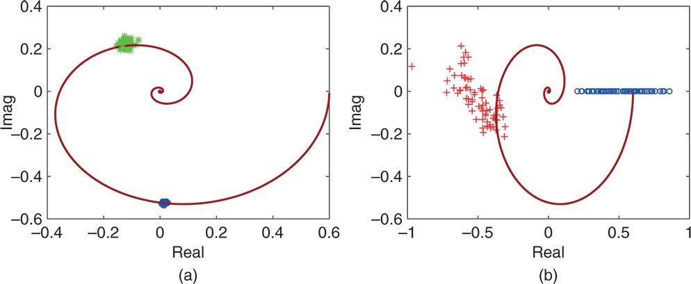
Figure 9.11 Frequency response estimation using FSF (Example 9.5).

9.4.4 Food for Thought

1. In the frequency estimation when using the FSF model and the relay feedback control data, we need to estimate the period in number of samples, . Why do you think that we identify the parameter using the maximum peak value of the FFT of the input signal? Can you propose an alternative approach to identify the parameter ?
2. What would happen to the frequency response estimation using FSF if the estimated parameter is wrong? Even so, would you still be able to get some estimation results?
3. Where are the poles of the frequency sampling filters? Can you express the frequency sampling filter model in terms of real coefficients instead of the complex coefficients?
4. Do you think that the estimated results from the recursive least squares estimation are identical to those obtained from the least squares estimation (see 9.17) with appropriately selected initial conditions?
5. What are the advantages when using the recursive least squares estimation?

9.5 Monte-Carlo Simulation Studies

In this section, we will further evaluate the estimation of the plant frequency response using the frequency sampling filter model in comparison with the estimation using Fourier analysis, where Monte-Carlo simulation studies are used.

The transfer function used in the Monte-Carlo simulation is

The relay amplitude is selected to be 1 and the sampling interval (s). The relay testing time is selected to be 800 (s). The noise used in the simulation is band limited noise with sampling interval (s) and power strength 1 together with a gain 0.02. In the Monte-Carlo simulation, the measurement noise is generated with a random seed that changes with each simulation to reflect the randomness of noise and its effect on the estimation results. The seeds used in the simulations are 0, 2,,60. Thus, there are 31 random seeds used in the Monte-Carlo simulation to generate the measurement noise. There is a small hysteresis in the proposed relay feedback control because the integral action acting as a low-pass filter has reduced the possible random switches caused by the noise.

9.5.1 Effect of Unknown Constant Disturbance

In many applications, during the relay experiments, there is an unknown constant disturbance. This type of disturbance often enters the system at the input variable, which is called the input disturbance. A typical example is the electrical load in an AC motor (Wang et al. (2015)). This type of disturbances will cause periodic oscillations in the relay feedback control to become unbalanced.

A constant input disturbance with magnitude of 0.3 is added to the relay feedback control experiments. Figure 9.12(a) shows the closed-loop relay feedback control responses in the presence of measurement noise and the input disturbance. From this figure it is seen that with the disturbance the oscillations are no longer in symmetry. Fourier analysis reveals [see Figure 9.12(b)] that the input signal has the fundamental frequency (rad), where and the next significant frequency in the periodic signal is followed by . By choosing the nine frequency parameters () and in the frequency sampling filter model, we obtain the estimated frequency parameters as shown in Figure 9.12(c). It is seen that the estimated parameters are unbiased with small variances, as shown through the Monte-Carlo simulations. In comparison, Figure 9.12(d) shows the estimated parameters using Fourier analysis, which are seen to have larger variances. The estimation results for frequency parameters at 0 and are not consistent when the oscillations are not symmetric caused by the constant disturbance.

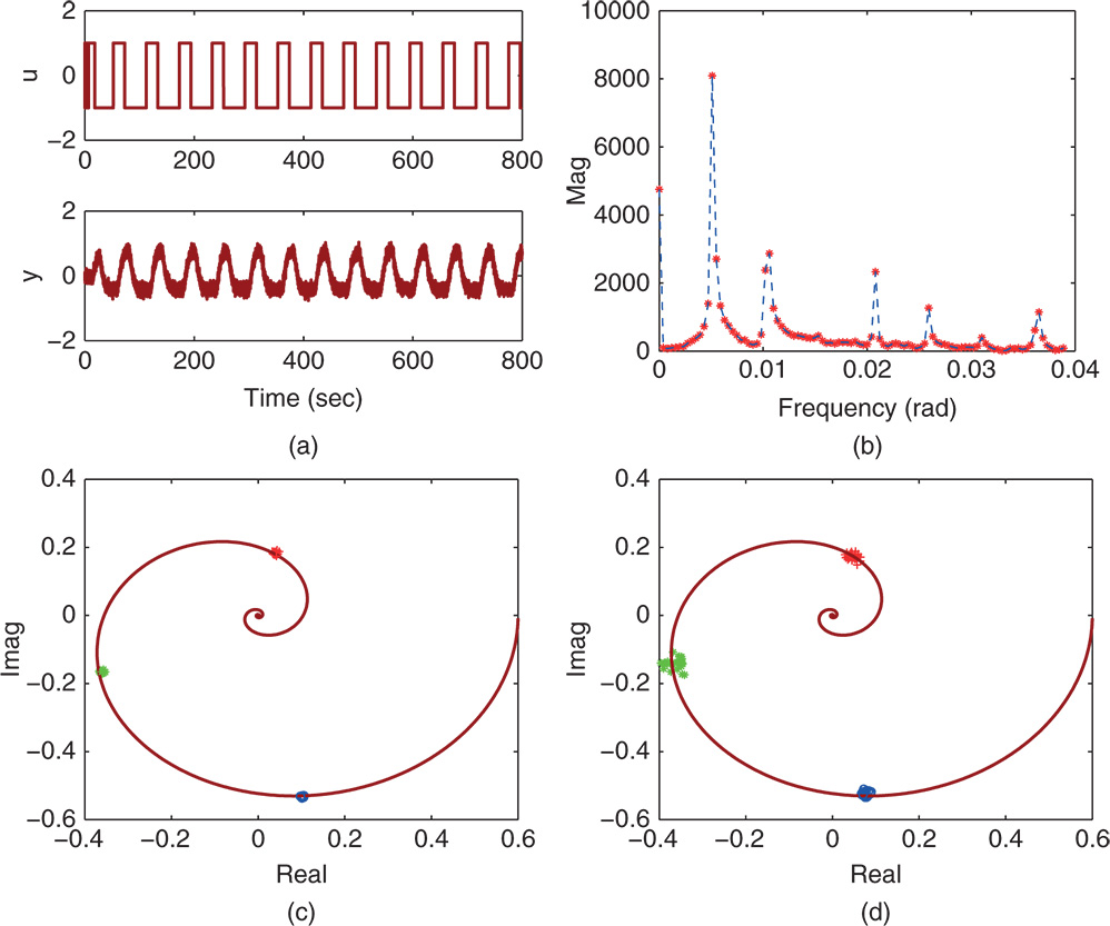
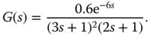
Figure 9.12 Monte-Carlo simulation results with random seeds in the presence of constant load disturbance. (a) Input and output signal. (b) Magnitude of DFT. (c) FSF estimation. (d) FFT estimation. Key: (solid line), o is the estimated values at , is the estimated values at , is the estimated values at .

9.5.2 Effect of Unknown Low Frequency Disturbance

In the application of process control, low frequency disturbances are frequently encountered. This group of studies will investigate what would happen to the relay feedback control and to the frequency response estimation in the presence of unknown low frequency disturbance.

In the Monte-Carlo simulation studies, the low frequency disturbance, entering into the system via the input signal, is generated by passing the same band limited measurement noise through a first order filter with transfer function:

which is then sampled using the same sampling interval (s). Note that the disturbance model has a time constant of 20 (s), which is much larger than the time constants of the system. Figure 9.13(a) shows the input and output data generated by the relay feedback control system. From this figure, it is interesting to see that the relay feedback control system no longer generates periodic oscillations in the presence of low frequency disturbances. This is confirmed through the Fourier analysis [see Figure 9.13(b)], from which only one spike in the magnitude of the Fourier transformation is observed. It is important to note that the relay feedback control system produces the oscillations that have the largest amplitude at 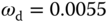, where 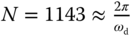. Figures 9.13(c) and (d) compare the estimation results obtained using the frequency sampling filter model and the Fourier analysis of the input and output data. It is seen from Figure 9.13(c) that the variances of the estimated parameters using the frequency sampling filter model are relatively small; however, there are small biases in the estimated parameters. In contrast, because the input signal is not periodic, the frequency response estimation using Fourier analysis produces poor results except the estimated parameters at , as shown in Monte-Carlo simulation studies, which is evident by the scatters on the complex plane [see Figure 9.13(d)].

Figure 9.13 Monte-Carlo simulation results with random seeds in the presence of unknown low frequency disturbance. (a) Input and output signal. (b) Magnitude of DFT. (c) FSF estimation. (d) FFT estimation. Key: (solid line), o is the estimated values at , is the estimated values at , is the estimated values at .

9.5.3 Estimation of the Steady-state Value

The final question to be answered in the Monte-Carlo simulation studies is whether the steady-state estimation will be valid using the frequency sampling filter model. Figure 9.14 shows that the estimation of steady-state information is not reliable when using relay feedback control. Depending on the particular seed of the noise generator, all the estimated steady-state gains vary significantly from the true value (0.6). The worst case is shown in Figure 9.14(b), where with the constant disturbance the steady-state gain estimated is 0.

Figure 9.14 Monte-Carlo simulation results for estimation of steady-state gain with random seeds. (a) Steady-state estimation (measurement noise). (b) Steady-state estimation (constant disturbance). (c) Steady-state estimation (low frequency disturbance). Key: (solid line), o is the estimated values at .

9.5.4 Food for Thought

1. The Monte-Carlo simulation studies presented in this section are based on integrator with relay feedback control. In the presence of constant disturbance, what is the role of the integrator played in the relay feedback control system? What are your observations in terms of the behavior of input and output signals?
2. In the presence of low frequency disturbance, has the integrator with relay feedback control tried to compensate the disturbance? Does this cause the breakdown of the periodicity of the input and output signals?
3. When there is a constant disturbance in the system, what kind of behavior would you expect from the input and output data for a relay with hysteresis? Do you expect accurate estimation results for this case when using FFT and FSF algorithms?
4. Why can not we consistently estimate the steady-state gain of the system using the data generated from the relay feedback control? Even for the case with low frequency disturbance?

9.6 Auto-tuner Design for Stable Plant

To design the auto-tuner for a stable plant, the integrator with relay feedback control is used to generate the input and output data for the frequency response identification because this configuration handles the measurement noise and disturbances well and also provides the valuable low frequency information for the PID controller design. We assume that the two estimated frequency response points from the relay testing data are the fundamental frequency , and , where is the number of samples within one period. Because of noise, the oscillation generated from the relay feedback control may not be perfectly periodic. Thus, the parameter is estimated using FFT analysis as illustrated in the previous sections (see Section 9.4). In the majority of the cases, the second frequency is selected as .

We assume that the plant transfer function is stable with all poles strictly on the left-half complex plane. Recall the desired closed-loop performance for the PID controller design using frequency response data in Chapter 8, which is specified through the control sensitivity function (see (8.18)), as

(9.20)

where is the desired closed-loop time constant, the parameter is selected so that is approximately equal to the dominant time constant of the system, is the steady-state gain of the system.

To link the PID controller design method to the auto-tuner, the question remains as how to choose the design parameters in (9.20). One possibility that works well is to derive the approximate dominant time constant of the system using the period of relay control, . For the majority of the system, it can be readily verified through simulation studies that the settling time of the system is roughly , namely half of the period under integrated relay control. With this knowledge, the dominant time constant of the process is selected about one-fifth of the settling time as

(9.21)

Now, one can choose the desired closed-loop time constant in relation to the dominant time constant of the process via the scaling parameter by defining

(9.22)

Substituting (9.21) and (9.22) into (9.20) leads to the desired control sensitivity function as,

(9.23)

hence, the desired closed-loop transfer function as

(9.24)

Note that in (9.24) the parameters and are known from the relay experiment and the user selected performance parameter is , which is the scaling factor between the estimated open-loop and the desired closed-loop time constants. This modification of the closed-loop performance specification leads to the automatic calculation of the PID controller parameters with minimum effort from the user.

Because the direct estimation of the steady-state gain is not consistent using the relay control experiment, an approximation is taken to yield a rough estimation of the gain as

where is the unknown steady-state gain of the system.

9.6.1 MATLAB Tutorial on Auto-tuner for Stable Plant

---

Tutorial 9.5

The objective of this tutorial is to implement the auto-tuner in a simulation environment. The system to be controlled has the following transfer function

Step by Step

1. Build a Simulink simulation program Tuner4StableSys.slx as shown in Figure 9.15, where the output data ports are the relay feedback error , the control signal and the output signal . The steady-state values and are set to zero. Inside the Configuration Parameters, the start time is selected as , stop time as , Solver option: fixed-step and ode4 (Runge-Kutta), Fixed-step size: Deltat. In the Simulink simulator, we have used the relay with integrator controller built in Tutorial 9.2. We can add noise and disturbance to the simulator for the different cases.
2. Create a new MATLAB file called Test4tuner.m and save it in the same directory as the Simulink simulator.
3. Define the system parameters using numerator, denominator and time delay . Enter the following program into the MATLAB file:

   num=0.6*[-6 1];
   den=conv([3 1],[2 1]);
   d=1; 

   

   Figure 9.15 Simulink diagram of auto-tuner for stable system.

4. Define the relay amplitude and hysteresis level, simulation time and sampling interval . Continue entering the following program into the MATLAB file:

   Ra=1; %relay amplitude
   epsilon=0.001; % hysteresis
   Deltat=0.05;
   Tsim=400;
   Nsim=Tsim/Deltat; 

5. Call the Simulink program to generate the three data output sets , and . Continue entering the following program into the MATLAB file:

   sim('Tuner4StableSys') 

6. Call the FSF estimation program created in Tutorial 9.4. Continue entering the following program into the file:

   [thetaCurrent,n,N]=FSFRelay(u,-e); 

7. Define the estimated frequency parameters. Continue entering the following program into the file:

   w1=2*pi/(N*Deltat);
   w2=6*pi/(N*Deltat);
   Gjw1=thetaCurrent(3);
   Gjw2=thetaCurrent(7); 

8. Find the estimated steady-state gain in approximation. Continue entering the following program into the file:

   K=abs(Gjw1); 

9. Define the ratio ( as an example) between desired closed-loop time constant in relation to the open-loop time constant, and the desired closed-loop time constant. Continue entering the following program into the file:

   beta=1;
   taucl=beta*0.1*N*Deltat; 

10. Call the FR4PID.m from Tutorial 8.1 to calculate the PID controller parameters. Continue entering the following program into the file:

    [Kc,tauI,tauD]=FR4PID(beta,taucl,w1,w2,Gjw1,Gjw2,K); 

11. Test this program with the closed-loop simulation as demonstrated in the next section and compare with results from Case B in the next section.

---

9.6.2 Evaluation of the Auto-tuner for a Stable Plant

In this section, we will firstly evaluate the closed-loop PID control performance of the proposed auto-tuner using four classes of systems commonly encountered in process control, and secondly perform comparative studies. For simplicity of the presentations, only measurement noise is added to the relay experiments. It has been verified that the auto-tuner will provide similar closed-loop performance when the constant disturbance or the low frequency disturbance are introduced during the relay experiments as long as we make an adjustment on the choice of the second frequency estimate for the PID controller design (see Sections 9.5.1 and 9.5.2).

There are four classes of systems used to evaluate the auto-tuner. Time delays are added for all testing cases to reflect the cases in process control. The same steady-state gain is used in all four cases for consistency in signal-to-noise ratio and the scaling of disturbance rejection in the closed-loop simulation. The sampling interval is , the relay amplitude is selected to be 1, and a measurement noise with standard deviation was added to the output. After the relay experiment, the number of samples for the period of the relay signal is calculated automatically to give the parameter , and the frequency responses at and are estimated. Then, by choosing , 1, and 2, three sets of PID controller parameters are calculated using the program FR4PID.m.

Case A. This is a testing case for high order systems. The transfer function of this system is given as

Case B. This is the testing case for systems with non-minimum phase behavior. The transfer function is given by

Case C. This is the testing case for systems with dominant time delay. The transfer function is given as

Case D. The final testing case uses an underdamped system, which has the transfer function

This transfer function has the damping coefficient . Thus, the system has oscillatory response in open-loop operation.

Relay feedback control is used to generate the input and output data for all four processes in the presence of measurement noise. Because of the integral action used in the relay feedback control, the measurement noise has not affected the input signal without using hysteresis in the design, and there is no correlation between the measurement noise and the input signal. This adds to the benefit of using an integrator in series with a relay control. The estimation of the frequency responses at and is performed using the frequency sampling filter model and the estimated frequency responses are accurate for all four cases.

9.6.2.1 PID Controller Parameters

By choosing , 1, and 2, three sets of PID controller parameters are calculated, which corresponds to the selection of three different desired closed-loop response speed. For instance, when , the desired closed-loop time constant is selected equivalent to half of the estimated dominant open-loop time constant. Table 9.1 shows the PID controller parameters of the four cases for the three values together with the mean squared errors, where the mean squared error is defined as , being the number of samples and being the error between the reference and output signals.

It is noticed that as increases, the proportional controller gain reduces, and the derivative gain reduces. In contrast, the variation of integral gain is smaller when changes.

9.6.2.2 Nyquist Plots

Figures 9.16(a)–(d) show the Nyquist plots of the four cases for the three control systems designed using , 1 and 2, where the frequency response of the system, , is used in the computation. It is seen from the Nyquist plots that the PID controllers with all three choices of lead to stable closed-loop systems. However, for , the closed-loop control systems for case B to case D had gain margins less than 2. As increases, both gain and phase margins for all four systems have increased. In particular, for the default choice of , the gain margins for all four case are greater than 2 and phase margins are greater than .

Table 9.1 PID controller parameters for different values.

Case
A	0.5		9.0098		0.0894
	1
	2
B	0.5		6.2732
	1
	2				0.1072
C	0.5
	1
	2
D	0.5
	1
	2				0.0543

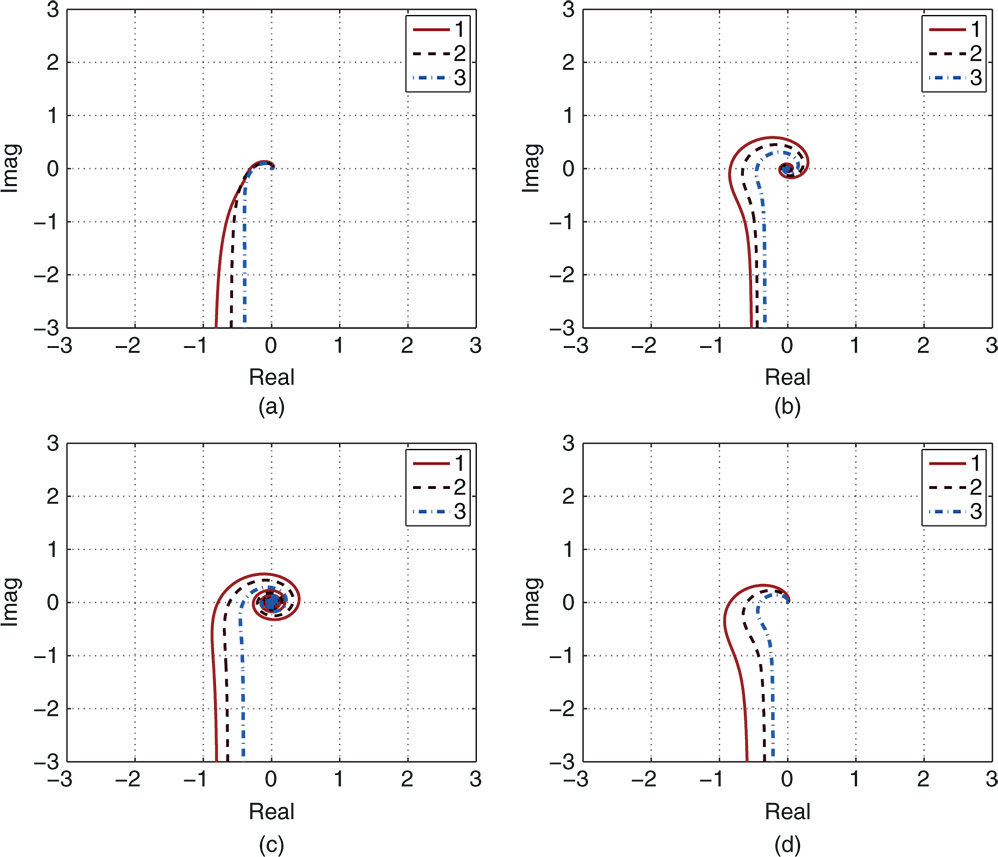
Figure 9.16 Nyquist plots using the PID controller parameters in Table 9.1. (a) Case A. (b) Case B. (c) Case C. (d) Case D. Key: line (1) ; line (2) ; line (3) .

9.6.2.3 Closed-loop Simulation Results

Closed-loop simulation is conducted for all four cases with , 1, and 2. In the closed-loop simulation, the derivative term is implemented on the output only and a derivative filter with time constant is used. A unit step signal is used as the reference signal at (s), and a unit step input disturbance enters at time (s). Figures 9.17(a)–(d) show the closed-loop simulation results for reference following and disturbance rejection. It is seen that all closed-loop systems are stable. The simulation results demonstrate that for a faster response to the reference signal, the PID control system will also have a faster response to disturbance rejection. The user can select the scaling parameter to achieve the desired closed-loop response as required. As increases, the closed-loop response speed reduces to both reference following and disturbance rejection. The overshoot in the reference response when is small could be overcome by using a two degree of freedom PID controller implementation as shown in Chapters 1 and 2.

Figure 9.17 Closed-loop simulation results using the PID controller parameters in Table 9.1. (a) Case A. (b) Case B. (c) Case C. (d) Case D. Key: line (1) ; line (2) ; line (3) .

9.6.3 Comparative Studies

In this section, we will benchmark the closed-loop performance of the PID controller found by the auto-tuner against the performance of the several other well known PID controllers. We will consider the following first order plus time delay model,

(9.25)

In the comparative studies, we will calculate the PID controller parameters using the IMC-PID controller design proposed by Rivera et al. (1986) (see Section 1.4.1), and the PID controller design by Padula and Visioli (2011) (see Section 1.4.2).

As in Chapter 1, the PID controller parameters using IMC-PID controller and Padula and Visioli tuning rules are calculated using the transfer function model (9.25). The PID controller parameters from the auto-tuner are calculated from the relay experiment where measurement noise with standard deviation of 0.02 was added.

In Table 9.2, we will choose two parameters to yield two sets of PID controller parameters from the auto-tuner. With this selection, it seems that all three PID controllers have a similar gain for the proportional control. However, the integral time constant varies between 26 and 35, and the derivative gain varies between 7 and 17. Figures 9.18(a)–(b) compare the three control signals and output signals in both reference following and disturbance rejection, which show that all three control systems have similar closed-loop performances in reference following and disturbance rejection.

Table 9.2 PID controller parameters and mean squared errors from the control simulation studies. Cases A and B use an auto-tuner, case C uses IMC-PID, cases D and E use Padula and Visioli PID.

Case	Spec.
A					0.1326
B
C
D			17.2991		0.1923
E		0.3205	22.5160	13.5770	0.1504

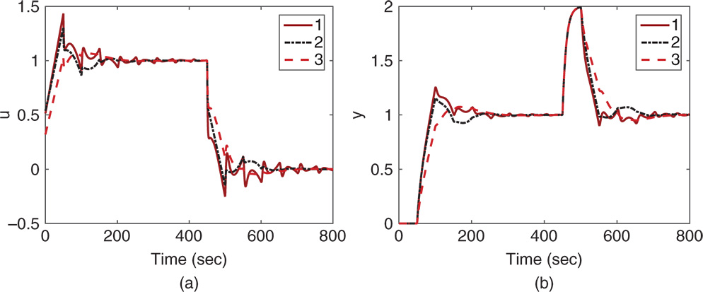
Figure 9.18 Closed-loop simulation results using the PID controller parameters in Table 9.2. (a) Control signal. (b) Output signal. Key: line (1) auto-tuner (); line (2) IMC-PID controller; line (3) Padula–Visioli design ().

9.6.4 Food for Thought

1. What are the key advantages when using the estimated frequency information directly for the auto-tuner design?
2. Can you propose an approach to convert the estimated frequency points to first order plus delay model, then design PID controller using the Padula and Visioli tuning rules given in Chapter 1?
3. If you wish to have a faster closed-loop response speed for disturbance rejection and reference following, should you increase or decrease the parameter ?
4. If the system has a large measurement noise, and you wish not to amplify it, should you increase or decrease the parameter ?
5. If the auto-tuner finds the derivative time constant to be negative, should we simply neglect the derivative term and implement the PI controller?

Figure 9.19 Block diagram of relay feedback control for an integrating system.

9.7 Auto-tuner Design for a Plant with an Integrator

For systems containing an integrator, in the design of auto-tuner for PID controllers, a proportional controller is first used to stabilize the plant. A relay with hysteresis element is utilized to generate the sustained oscillation for the closed-loop control system. The block diagram of the relay feedback control for an integrating system is illustrated in Figure 9.19.

9.7.1 Estimation of an Integrating Plus Delay Model

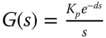
The approximate model of an integrating system is assumed to be of the following form:

(9.26)

For most physical systems, there are more or less approximations involved in obtaining the integrating plus time delay model. For an integrating plus time delay system, a single frequency is sufficient to determine its gain and time delay . Therefore, it is exceedingly simple to obtain an integrating plus delay model using the relay feedback control experimental data.

As shown in Section 9.4, the estimation of the closed-loop frequency response using either FFT analysis or an FSF model will yield the information where is the estimated closed-loop frequency response and is the fundamental frequency of the relay feedback control.

With the knowledge of the proportional controller , the frequency response of the plant is calculated from the closed-loop frequency response relationship,

leading to

(9.27)

Now, letting the frequency response of the integrating plus delay model (9.26) be equal to the estimated leads to

(9.28)

Equating the magnitudes on both side of (9.28) gives

(9.29)

where . Additionally, from (9.28), the following relationship holds:

This gives the estimate of time delay as

(9.30)

In the event that parameter is negative, its absolute value is taken as the estimated time delay.

It is seen here that if the system is approximated by integrating with the time delay, the plant information at a single frequency is sufficient to determine the plant gain and time delay.

9.7.2 Auto-tuner for Integrating Systems

On obtaining the estimated integrating plus time delay model (9.26), one can find the PID controller using the empirical rules such as the modified IMC-PI controller in Skogestad (2003), which was discussed in Section 1.4.1, or tuning rules in Tyreus and Luyben (1992). We will use the empirical rules presented in Section 8.4.3, which gives the flexibility of PI, PID and PD controllers together with the gain margin and phase margin for the selection of performance parameter .

One is encouraged to follow Tutorial 9.1 for the relay feedback control and Tutorial 9.4 for the estimation of the frequency response using an FSF so as to validate the following simulation example.

The following example is to show the behaviour of the auto-tuner when it is applied to a complex integrating system.

---

Example 9.6

Consider the design of PID controller using auto-tuner for the integrating system described by the following transfer function:

(9.31)

The proportional feedback control gain is selected as to produce a stable system for the relay experiments. The relay amplitude of and hysteresis of are chosen. Find the PID controller parameters for and . In the relay feedback control, band limited white noise is added to the output, where the signal power is selected to be with gain and seed .

Solution. Figure 9.20 shows the input and output data with the relay feedback control. Using the frequency sampling filter model, the closed-loop frequency response is estimated as

and the plant frequency response is estimated using (9.27) as where . Figure 9.21 compares the estimated frequency response at against the frequency response of the plant transfer function (9.31). It is seen that the estimated result is quite accurate.

Figure 9.20 Input and output relay feedback control data (Example 9.6).

Figure 9.21 Comparison between the estimated frequency point with the original frequency response (Example 9.6). Key: solid line, plant frequency response; dot, estimated frequency response.

With the single frequency response point, the integrating time delay model is found using (9.29) and (9.30):

(9.32)

This model leads to the PID controller parameter using the empirical rules in Section 8.4.3 as

Because the original system actually contains an integrator, the Nyquist diagrams (see Figure 9.22) show their frequency responses are very similar at the cross over frequency region as well as low and medium frequency regions, comparing the PID controller applying to the integrating plus delay model (9.32) with that applying to the original system (9.31). Figure 9.22(b) compares the magnitudes of their sensitivity functions. It is seen that the discrepancies are very small between the sensitivity functions in all the frequency regions. The PID control system performance is evaluated with a step reference signal and a step disturbance signal entering the simulation at (s). The derivative control is implemented on the output only with the filter time constant equal to . Three control configurations are considered (see Figures 9.23(a) and (b)). Overall, the PID controller produces the best performance in terms of disturbance rejection. The PD controller could not reject the step disturbance; however, it produces the best reference following performance. There is an oscillation in the closed-loop control if a PI controller is used.

Figure 9.22 Frequency response comparison (Example 9.6). (a) Nyquist diagram. (b) Sensitivity function. Key: line (1) frequency response calculated with integrating plus delay model; line (2) frequency response calculated with the actual plant.

---

Although it is derived for an integrator plus delay system, the auto-tuner provides satisfactory closed-loop performance for many classes of systems. This is illustrated by the following example.

---

Example 9.7

Assume that a second order system with time delay is described by the transfer function:

(9.33)

Figure 9.23 Comparison of closed-loop performance for three types of controllers (, ). (a) Control signal. (b) Output. Key: line (1) PID control response; line (2) PI control response; line (3) PD control response.

Figure 9.24 Input and output relay feedback control data (Example 9.7).

Choosing the proportional feedback control gain , and relay amplitude of and hysteresis of , find the PID controller parameters for and . In the relay feedback control, band limited white noise is added to the output, where the signal power is selected to be with gain and seed .

Solution. Following Tutorial 9.1, we obtain the relay control data for the proportional controlled system as shown in Figure 9.24. Then, following Tutorial 9.4, the closed-loop frequency response with proportional control is estimated using the FSF model as

and the plant frequency response is estimated using (9.27) as where . Figure 9.25 compares against the plant frequency response produced by the original system (9.33). It is seen that despite of the measurement noise, the estimation result is very accurate. With the frequency response information, the integrator plus time delay model becomes

(9.34)

based on (9.29) and (9.30).

Figure 9.25 Comparison between the estimated frequency point with the original frequency response (Example 9.7). Key: solid line, plant frequency response; dot, estimated frequency response.

Figure 9.26 Comparison of closed-loop performance for three types of controllers (, ). (a) Control signal. (b) Output. Key: line (1) PID control response; line (2) PI control response; line (3) PD control response.

By choosing , the PID controller parameters are found using the empirical rules in Section 8.4.3:

This PID control system is simulated using a unit step input reference signal with sampling interval s. A step input disturbance with amplitude enters the simulation at half of the simulation time. Figure 9.26 shows the evaluation results for the configurations of PID, PI, and PD control systems. In the implementation, the derivative control is implemented on output only with a filter time constant , both proportional and integral control functions are implemented on the feedback error. The PID controller provides much improved performance over the PI and PD control systems for this choice of parameter. The oscillation for the PI control system reduces when is increased. In general, if a PI controller is used, the parameter should be selected to be larger than to reduce the oscillation due to the small phase margin, which can be verified for this example.

To understand why the auto-tuner designed for the integrating system worked for a stable system, a frequency response analysis is performed. Figure 9.27(a) makes a comparion between the Nyquist diagrams of the controller with the estimated integrating plus delay model (9.34) and the controller with the stable plant transfer function (9.33). The Nyquist diagrams show that their frequency responses are quite similar at the cross over frequency region, which produces the closed-loop stability with sufficient gain and phase margins when the controller found by the auto-tuner is applied to the original system. Figure 9.27(b) compares the magnitudes of their sensitivity functions. It is seen that at the high frequency region, they are very similar. However, at the lower and medium frequency regions, there are some discrepancies. In particular, in the lower frequency region, the magnitude of the sensitivity is much smaller when the controller is applied to the original system, which indicates that the controller may have a better disturbance rejection when it is found using the auto-tuner designed for the integrating systems.

---

This auto-tuner will be used for finding the PID controllers for the unmanned aerial vehicles in Chapter 10.

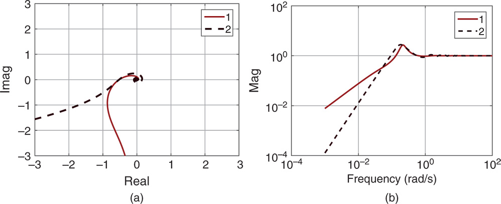
Figure 9.27 Frequency response comparison (Example 9.7). (a) Nyquist diagram. (b) Sensitivity function. Key: line (1) frequency response calculated with integrating plus delay model; line (2) frequency response calculated with the actual plant.

9.7.3 Auto-tuning of Cascade Control Systems

Auto-tuners are very convenient for tuning cascade control systems. The inner-loop control system will be auto-tuned first to find the appropriate controller, followed by the implementation of this secondary controller. An outer-loop control system will be auto-tuned with the closed-loop secondary system considered. As an illustration, we consider the following example.

---

Example 9.8

The transfer function for the secondary system is assumed to have the transfer function:

(9.35)

The transfer function for the primary system is described by

Find the PID controllers using the auto-tuner for the cascade PID control system.

Solution.

Auto-tuning inner-loop controller

The proportional controller used to stabilize the inner-loop system is selected to be . In the simulation, a zero mean white noise with standard deviation of is added to the measured output. The relay amplitude is selected to be and hysteresis is to prevent the relay from the switching caused by the random noise. Figure 9.28 shows the input and output data for the closed-loop system. It is seen from this figure that the measurement noise has caused some random switches of the relay, particularly in the beginning of the simulation. From the relay testing data, the number of samples within one period is estimated to yield . The estimated fundamental frequency response for the closed-loop system with is . From this value, the frequency response of the integrating system is found as . With the frequency response value of the inner-loop system, the following integrator with delay model is calculated based on (9.29)–(9.30):

Figure 9.28 Relay feedback control signals from inner closed-loop system (Example 9.8). top figure input signal; bottom figure output signal.

Choosing , which gives the desired closed-loop time constant about , with PID controller tuning rules presented in Section 8.4.3, the PID controller parameters for the inner-loop control system are calculated as

Considering that the value is quite small, also noise in the system, the inner-loop controller is selected as a PI controller. The Nyquist curve for the PI controller against the original system described by (9.35) is shown in Figure 9.29(a). Roughly it can be read from the figure that the control system has gain margin about and phase margin about degree, which are quite close to the specification in the tuning rules. The inner-loop PI control system is evaluated via a step change at time and a step input disturbance with amplitude 0.05 entering the system at (sec). Figure 9.29(b) shows the control signal response and the output response to the reference change and the disturbance.

Auto-tuning outer-loop controller

The automatic tuning process is repeated for the outer-loop control system, however, the inner-loop system is controlled with the PI controller auto-tuned previously. It is important for a cascade control system in the relay experiment that the inner-loop dynamics are considered. In the outer-loop relay experiment, the proportional controller is used to stabilize the primary system, which has an integrator. The relay feedback control data with amplitude of and hysteresis of for the outer-loop system is shown in Figure 9.30 where the same measurement noise is added. It is seen that there are many more random switches due to the measurement noise. The estimation of the closed-loop frequency response using the frequency sampling filter model leads to the value at the fundamental frequency. Then, the calculated frequency response of the primary plant together with the inner-closed-loop system at the fundamental frequency of the relay signal is .

Figure 9.29 Auto-tuning inner-loop control system (Example 9.8). (a) Nyquist curve with . (b) Closed-loop response.

Figure 9.30 Relay feedback control signals from outer- closed-loop system (Example 9.8). top figure input signal; bottom figure output signal.

The integrator with time delay model for the design of primary controller is derived using (9.29)–(9.30) to give:

Note that the original time delay for the primary plant is , however, because of the inner-loop dynamics, the estimated time delay is over . By choosing , which gives the desired closed-loop time constant about , the PID controller parameters are calculated using the tuning rules to give

By neglecting the derivative control term, the PI controller is determined for the outer-loop control system. Figure 9.31(a) shows the Nyquist curve for the cascade control system with the primary controller auto-tuned. It is seen that the closed-loop system has gain margin approximately greater than and phase margin greater than degree. The cascade control system is finally evaluated by using a step reference signal at and a step disturbance with magnitude of entering at as the input disturbance to the secondary plant. Figure 9.31(b) shows the cascade closed-loop control system to the reference signal and the disturbance signal.

Figure 9.31 Auto-tuning outer-loop control system (Example 9.8). (a) Nyquist curve with . (b) Closed-loop response.

---

9.7.4 Food for Thought

1. Why do you think that the auto-tuner designed for integrating system can be applied to a stable system?
2. Do you expect that this class of auto-tuners would produce a faster disturbance rejection based on the observation of the sensitivity function in Example 9.7?
3. We use relay with hysteresis in the identification experiments. Do you think that it would work better if we use the integrator with relay control apparatus in the identification experiment? Why?
4. If you wish to have a faster closed-loop response for disturbance rejection, should you increase or decrease the parameter ?
5. If you wish to reduce the effect of measurement noise, should you increase or decrease the parameter ?

9.8 Summary

We have discussed automatic tuning of PID controllers in this chapter. The auto-tuners are designed for stable systems and integrating systems. Both involve relay feedback control to generate the input and output data for estimation of plant frequency response. Then, the PID controller design methods discussed in Chapter 8 are used to automatically find the controller parameters.

The other important aspects of the chapter are summarized as follows.

• Relay feedback control is utilized in generating the input and output data for estimation of process frequency response. Following the MATLAB tutorials, we can create our own Simulink functions for simulations of relay feedback control system and those programs can also be translated into C-program for micro-controller implementation.
• The input and output data collected from the relay feedback control experiments in simulation or in real-time implementation are used for the estimation either using Fourier analysis or using the frequency sampling filter model. The frequency sampling filter based estimation is performed in a recursive least squares algorithm with the feature for real-time applications.
• Monte-Carlo simulation studies have been used to investigate the accuracy of the estimated models in the presence of measurement noise and low frequency disturbances.
• Once the process frequency response is estimated, the PID controller design methods either using two frequency points or using an integrating with delay model are applied to obtain the PID controller parameters.

9.9 Further Reading

1. Relay feedback control has been one of the key instruments used in the automatic tuning of PID controllers (Astrom and Hagglund (1984), Astrom and Hagglund (1988), Astrom and Hagglund (1995), Astrom and Hagglund (2006), Hagglund and Astrom (1985), Yu (2006), Johnson and Moradi (2005)).
2. The auto-tuner for stable systems was originally presented in Wang (2017).
3. Auto-tuners are experimentally compared in laboratory test beds (Berner et al. (2018)).
4. Books for automatic tuning of PID controllers include Yu (2006), Sung et al. (2009)
5. Software package introduced for tuning of PID controllers is discussed in Oviedo et al. (2006). Use of phase-locked-loop idea is used to auto-tune PID controllers in Crowe and Johnson (2002).
6. Auto-tuners in closed-loop operations include Lee et al. (1990), Schei (1992), Tan et al. (2000). Automatic tuning of cascade PID control system was discussed in Jeng and Lee (2012) and Jeng (2014). Automatic tuning of PID controller for nonlinear systems was presented in Cetin and Iplikci (2015). Multi-loop PID controller tuning was proposed using an optimization based approach (Dittmar et al. (2012)). A simplified approach to auto-tuner design with respect to disturbance rejection was proposed in Romero et al. (2011). An auto-tuner was designed for fractional order plus delay model in Jin.
7. Estimation of transfer function model by changing between two relay feedback controllers to obtain multi-frequency signals (Schei (1994)), and estimation of step response model (Wang and Cluett (1997a)).
8. Frequency sampling filters was introduced in Bitmead and Anderson (1981) and Wang and Cluett (2000).
9. The auto-tuning algorithm presented in this chapter has been successfully used to attitude control of fixed-wing unmanned aerial vehicle with experimental validations (Poksawat et al. (2016), Poksawat et al. (2017) and Poksawat (2018)). It has been used to find a PID control system for an electro-mechanical system with two inputs and two outputs (see Wang et al. (2017)). In Chen (2017), the auto-tuning algorithm has been successfully used to find flight controllers for quadrotor UAVs.
10. There are many books for the topics of system identification (see Ljung (1999), Soderstrom and Stoica (1989), Goodwin and Sin (1984), Young (2012), Soderstrom (2018)).

Problems

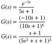
1. 9.1 Consider the systems with the following transfer functions:
   
   1. Suppose that the measurement is corrupted by a noise source that has zero mean with variance 0.1. Following Tutorial 9.1, write the RelayH.slx real-time function and build a Simulink relay feedback control simulation program. Sampling interval .
   2. Choose the relay amplitude to be and adjust the hysteresis level to prevent the random switches caused by the noise. Apply the relay feedback control program to the above systems. What are your observations on the choice of with regard to relay amplitude and the magnitude of the measurement noise? If you use Simulink noise generator in the continuous-time, will the sampling interval affect the choice of ?
   3. Add a constant input disturbance with amplitude of to the relay feedback control. What are the effects of this disturbance on the relay with hysteresis control system?
2. 9.2 Consider the three systems given in Problem 9.1.
   1. Following Tutorial 9.2, write the MATLAB real-time function RelayI.slx for relay with integrator control. Choose the same relay amplitude with very small hysteresis ().
   2. Apply the relay with integrator control to the three systems given in Problem 9.2. What are your observations on the effect of noise with this type of relay feedback control system?
   3. Add a constant input disturbance with amplitude of to the relay feedback control. What are the effects of this disturbance on the relay with integrator control system?
   4. Will the sampling interval affect the relay with integrator control system?
3. 9.3 Assume that we have generated relay feedback control data by solving Problem 9.1.
   1. Following Tutorial 9.3, write the MATLAB program FFTRelay.m for estimation of frequency response using relay feedback data.
   2. Apply the program to the six sets of data generated from Problem 9.1.
   3. Evaluate the estimation results against the Nyquist curves obtained from the transfer functions.
   4. What are your observations on the effect of measurement noise on the accuracy? The effect of constant input disturbance?
   5. Alternatively, following Tutorial 9.4, write the MATLAB program FSFRelay.m for the estimation of frequency response using relay feedback data and repeat the exercises outlined in the previous steps.
4. 9.4 Apply the MATLAB program FFTRelay.m (or FSFRelay.m) to the six sets of data generated from Problem 9.2, where relay with integrator control has been used. What are your observations on the effect of measurement noise and disturbance on the accuracy of the estimation?
5. 9.5 Consider the systems with the following transfer functions:
   
   1. Following Tutorial 9.5, write the auto-tuner for stable systems.
   2. Apply the auto-tuner to the above systems with appropriate sampling interval , where the performance parameter .
   3. Evaluate the closed-loop performance with a unit step reference signal and a step input disturbance with magnitude of .
   4. What are your observations on the closed-loop responses to reference following and disturbance rejection in terms of the parameter ?
   5. Add measurement noise and the input disturbance in the relay with integrator control system. Will the noise and disturbance significantly affect the performance of the closed-loop control system produced by the auto-tuner?
6. 9.6 Consider the integrating systems with the following transfer functions:
   
   1. Following the computational steps outlined in Section 9.7, write the auto-tuner for integrating systems where the relay with hysteresis is applied to a proportionally controlled system (see Figure 9.19).
   2. Choose a proportional controller that will produce a stable closed-loop system and apply the auto-tuner to the above systems, where sampling interval , relay amplitude and hysteresis are selected appropriately.
   3. Evaluate the closed-loop control system performance with unit step reference signal and a step input disturbance with amplitude for the performance parameter .
7. 9.7 The auto-tuner derived for integrating system can also be applied to stable systems in a closed-loop controlled environment. Considering the systems with the following transfer functions
   

   Use the auto-tuner with integrator model to find the PID controller parameters for these systems. In the relay control experiments, feedback control gain , and relay amplitude of and hysteresis of are used. Sampling interval is selected. The performance parameters and are selected for fast disturbance rejection. Evaluate the closed-loop control system performance for step input disturbance rejection with a disturbance amplitude of .

8. 9.8 The auto-tuners are very convenient for tuning cascade control systems. Consider that a cascade control system has the inner-loop transfer function
   

   and the outer-loop transfer function

   
   1. Construct an auto-tuner for this cascade control system from tuning the inner-loop control system first followed by tuning the outer-loop control system.
   2. By choosing the closed-loop performance parameter , the closed-loop response speed can be specified for the inner-loop and outer-loop control systems. In order for the cascade control system to work properly, the inner-loop response speed needs to be much faster than the outer-loop's response speed. How do you choose for this auto-tuned cascade control system?
9. 9.9 We can design an auto-tuner for integrating systems using the modified IMC-PI controller introduced in Skogestad (2003), which was discussed in Section 1.4.1. For the estimated integrating with delay model, , the PI controller parameters are calculated using the following expressions:
   

   Repeat the exercises given in Problem 9.7 with the closed-loop performance parameter . What are your observations when you compare these two PI control systems?

Note

1. 1   One can choose the parameter lam to be less than 1 for time varying systems (see Goodwin and Sin (1984), Young (2012), Ljung (1999)).