8
PID Controller Design for Complex Systems
8.1 Introduction
The PID controller design methods discussed in the previous chapters are either model based approaches or rule based approaches. It is clear that when using a model based approach, a first order model yields a PI controller and a second order model yields a PID controller. In some applications, the first order and second order models are basically an approximation to the actual physical systems. In other applications, the underlying physical systems are complex and are of higher order. This chapter studies how to design PID controllers for higher order systems directly using frequency response data.
8.2 PI Controller Design via Gain and Phase Margins
This section presents PID controller design via specification of gain margin and phase margin.
8.2.1 PI Controller Design Using Gain Margin and Phase Margin Specifications
The starting point is to assume that the frequency response of a desired open-loop transfer function  at a specific frequency point
  is available. It is also assumed that the frequency response of the system
  is available at
  .
.
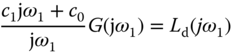
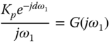
At the frequency  , the actual open-loop frequency response with a PI controller is

Letting the actual open-loop frequency response equal its desired counterpart leads to
which is

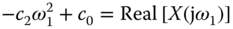
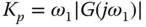
Comparing the left-hand side with the right-hand side of (8.2) gives


From  and
and  , the PI controller parameters are calculated using the following relationships
One of the choices for the frequency response of a desired open- loop transfer function  is to specify the gain margin for the PI control system. Say, if one wishes to have a gain margin of 2, then
  . However, the frequency
  still needs to be determined, where
  in this specification is the cross-over frequency for the desired closed- loop system. Had a proportional controller
  been used in the design,
  could be chosen as the cross-over frequency for the
  . Following the same practice, because of the
  phase-lag introduced by the integrator in the controller, a reasonable practice is to select
  in the vicinity of the frequency
  where
where  for the first time crosses the imaginary axis. Note that
  because at
  ,
,  , consequently resulting in
  . A practice is to set
  .
.
Similar to the specification of the desired gain margin, the phase margin can also be used to specify the desired open-loop frequency response  . It is known that
  at the frequency (say
  ) that defines the phase margin. Hence, by denoting the phase margin as
  , then
8.2.2 Design Examples
The following example demonstrates the performance of the PI controller when using gain margin and phase margin specifications.
The following example is to show how the PI controller is used to control a higher order complex system with time delay, which is very difficult if other design methods are used for this case. The closed-loop performance when using the specification of gain margin is left as an exercise (see Problem 8.1).
It must be emphasized that the PI controller design using the specification of either gain margin or phase margin does not work for severely underdamped systems and unstable systems. This is because for these classes of systems, the desired open-loop frequency response  must be calculated in a more sophisticated way to reflect the undesired process characteristics. Problem 8.1 is left for the verification of these statements.
8.2.3 Food for Thought
- If we are to fit the frequency response of a higher order transfer function with a first order plus delay model or a second order plus delay model, how would you propose to estimate the time delay parameter
 ?
? - Would you say that the stability of the closed-loop system is not guaranteed when a PID controller is designed using an approximate model?
- Is it correct that the closed-loop stability is checked against the original higher order system?
- If the amplitude of the frequency response of the original system,
 , asymptotically decays as
  increases, do you think that the PI controller design methods using the specification of gain margin or phase margin will guarantee closed-loop stability for the original system?
 - Will the amplitude of the frequency response of the original system containing a pair of underdamped modes asymptotically decay as
 increases?
8.3 PID Controller Design using Two Frequency Points
This section discusses an intuitive and simple approach to PID controller design from the perspective of curve fitting of the frequency response of the loop transfer function.
8.3.1 Finding the PID Controller Parameters
As we know from the PI controller design, the process frequency response information at one frequency  is sufficient to find the two parameters (
 and
and  ). Because there are three parameters contained in a PID controller, naturally it requires the process frequency response information at two frequencies
  and
and  (
( ) to uniquely determine the three parameters (
 ,
,  and
and  ).
).
The starting point is to assume that the desired open-loop frequency response  is specified at
  and
and  , and the plant frequency response
  is also known at
  and
and  . Furthermore, we assume that
  . The specifications of the
  , and the frequency points
  and
and  will be discussed later.
For a PID control system, the actual open-loop frequency response at  is
is

and at  is
is

Thus, by letting

and comparing their real and imaginary components, the following linear equations hold:

where for notational simplicity,


From (8.9), the coefficient  is calculated as

From (8.10) and (8.11), the coefficients  and
and  are calculated by solving the two linear equations, giving
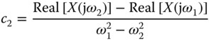

Finally, the PID controller parameters are given in relation to  as
as
Because there are two frequencies  and
and  used in the design, more thought is required in the selection of not only
  at
at  and
and  , but also the frequencies
  and
and  themselves. Naturally, one assumes that the desired gain margin and phase margin are good candidates for the selection of
  . However, the challenge is to find the suitable values for the desired gain margin and phase margin together with
  and
and  .
.
The following example is used to demonstrate the difficulties in specifying  .
.
8.3.2 Desired Closed-loop Performance Specification using Two Frequency Points
It is apparent that the desired closed-loop performance specification via choice of  plays an important role in the design of a PID controller using the frequency response. The parameters such as gain margin and phase margin are relatively easy to specify in terms of closed-loop stability; however, it is difficult to relate them to the actual closed-loop response performance for reference following and disturbance rejection.
Going back to the drawing board, it is necessary to find a systematic and yet a simple way to specify  such that the closed-loop response performances for reference following and disturbance rejection are met. Another aspect in PID controller design apart from the performance specification is that, because of the limited complexity of the controller structure, there is a difference between what is desired and what is achievable. In other words, what we ask for in a PID control system is not necessarily achievable.
One of the effective ways to specify the desired open-loop frequency response  is via the specification of the desired frequency response of the complementary sensitivity function
  , where

Hence, if  is specified, then
  is calculated as

The properties of  are directly related to reference following and noise attenuation, as well as indirectly to disturbance rejection via the frequency response of the desired sensitivity function

What are the key characteristics of a complementary sensitivity function? There are four basic characteristics listed as below.
- The desired complementary sensitivity function
 must have all poles on the left-hand side of the complex plane.
 - With a PID controller in the feedback control, the complementary sensitivity
 must be equal to unity at
  .
. - The plant unstable zeros contained in
 will be in the presence of
  because the plant unstable zeros cannot be changed through feedback control.
 - The plant time delay
 will appear in the desired complementary sensitivity function because the plant time delay can not be changed through feedback control.
All the characteristics can be easily verified with closed-loop transfer function calculations, which is left as an exercise.
In view of these characteristics of the desired complementary sensitivity function, without a complete knowledge about the system transfer function  , it could be a difficult task to choose a suitable
  in its own right. This task could become even more difficult when the plant frequency information
  is given at one or two frequency points.
The specification of  is proposed as follows so that the PID controller design using frequency response data remains effective while maintaining the original simplicity. This specification was originally proposed in Wang et al. (1995b) and was described in more detail in Wang and Cluett (2000).
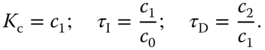
We assume that the plant transfer function  is stable with all poles on the left-half complex plane and the system has no severely underdamped poles. With these assumptions, the behaviour of a control signal to a step reference signal in an over-damped closed-loop control system can be approximated by a first order response. This behaviour is then described by the desired control sensitivity function
  with the first order transfer function:

where  is the desired closed-loop time constant for the control signal, the parameter
  is selected so that
  is approximately equal to the dominant time constant of the system,
  is the steady-state gain of the system. When the dominant time constant of the system is unknown, which is the case for using the plant frequency response data in the design, the parameter
  is a tuning parameter.
The desired complementary sensitivity function follows from the desired control sensitivity function in the form:
Clearly,  is stable as
  and the transfer function
  is assumed to be stable;
  at steady-state (
 ) is equal to unity because of the factor
  , where
  is the steady-state gain of
  ; and the time delay or zeros in
  are contained in
  . Therefore, all four characteristics of
  have been included in this simple specification.
If the dominant time constant of the plant is estimated (or known) as  , then the desired closed-loop time constant
  is chosen to be
  , where
  .
.
8.3.3 Design Examples
8.3.4 MATLAB Tutorial on PID Controller Design Using two Frequency Points
The objectives of the following two tutorials are to produce a MATLAB program for PID controller design using two frequency response points (see Tutorial 8.1) and to test this program using a simulation example (see Tutorial 8.2).
The program needs to be tested so that we can use it for applications.
Closed-loop simulation of the PID control systems are performed using a derivative filter with the filter time constant being  . Both the proportional control term and derivative control term are implemented on the output only. Figure 8.6 shows the closed-loop responses for reference following of a unit step signal and disturbance rejection. The input step disturbance with amplitude of 2 enters the system at
  (s). It is seen that by increasing
  , the closed-loop response speed is reduced, however, the slight oscillation with the smaller
  is overcome.
Note that the MATLAB program FR4PID.m will be used for auto-tuner design in Chapter 9 where the plant frequency information at  and
and  will be found by the relay feedback experiments. Additionally, the PID controller will degrade to a PI controller if the derivative gain
  is either negative or is too small. In the case of the PI controller, the proportional gain
  and
and  remain unchanged from the calculation of the FR4PID.m program.
8.3.5 PID Controller Design for Beer Filtration Process
In the work by Lees and Wang (2015), two transfer function models were estimated for a beer filtration process at different operational conditions.
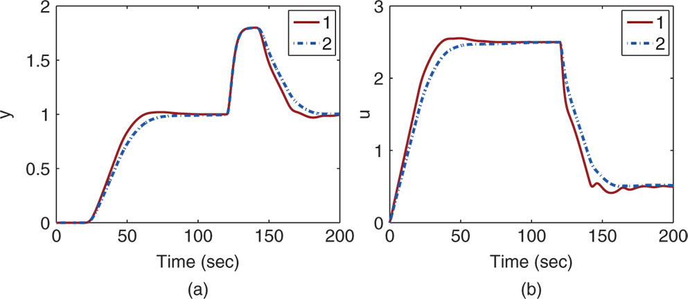
Figure 8.6 Comparison of closed-loop responses of PID control systems. (a) Output response. (b) Control signal. Key: line (1)  and
and  ; line (2)
  and
and 
For the first operational condition, step response experiments were conducted to obtain the estimated transfer function:

For the second operational condition, the estimated transfer function is
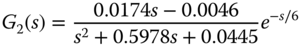
where the time unit for the transfer functions is minute, instead of second. The filtration process is clearly a nonlinear system, in which the system dynamics change with respect to operating conditions.
In order to design a single PID controller for the system, the frequency responses of the transfer function models are then averaged point-by-point. Figure 8.7 shows the frequency response of  ,
,  and the averaged frequency response
  . To obtain the two frequency response points
  and
and  , the real and imaginary parts of
  are examined, where
  is identified as the point when the real part of
  changes sign from negative to positive and
  is identified as the point where the imaginary part changes sign from positive to negative. The corresponding frequency response
  at
at  is
is  and at
  is
is  .
.

Figure 8.7 Frequency response. Key: line (1)  ; line (2)
  ; line (3)
The desired closed-loop performance is specified at  and
and  through the following relationship:
where  ,
,  and
and  . Note that we have selected
  , which corresponds to the dominant time constant of
  .
.
Using the MATLAB function FR4PID.m produced in Tutorial 8.1, we calculate the PID controller parameters:

Figure 8.8 shows the frequency response  and
and  , from which we can estimate that the closed-loop control systems have the minimum gain margin of 2 and phase margin
  .
.
In the closed-loop simulation, the PID controller is discretized and a derivative filter with time constant  is added to the derivative term to avoid amplification of measurement noise. The discretized control signal ready for implementation is calculated using ((4.40)) in Chapter 4. Additionally, the control signal is computed with quantization for the possible implementation of the control system by a plant operator. The control signal with quantization is chosen to be a multiple of 0.01, which corresponds to 1 percent change in the control signal as the basis unit. Also, if the calculated control signal change
  is less than 1 percent, then the control signal remains constant.
The control objective is to maintain a constant output  , and due to the filtration operation, it drops with respect to time. The closed-loop control system is simulated with an output disturbance added to the system while maintaining a constant reference response. The typical case of the disturbance mimics the situation where the
  reduces in a series of step changes. Because of the nonlinearity, the same PID controller is used to control both
  and
and  in the simulation studies. Figure 8.9 shows the control signal response and output response to the output disturbance in a series of steps. It is seen that the closed-loop PID control has maintained the constant output value despite of the disturbance. Note that with the same filter, but at different operational time,
  has a smaller steady-state gain, corresponding to the filter condition deteriorating. As a result, a larger steady-state control signal is required to maintain the same operational conditions. This is evident from comparing the control signals in Figure 8.9 (a).
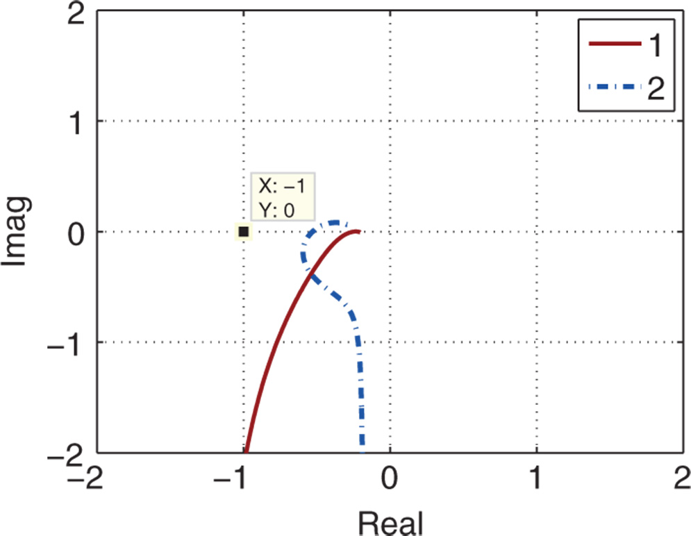
Figure 8.8 Nyquist plot. Key: line (1)  ; line (2)
  .
.
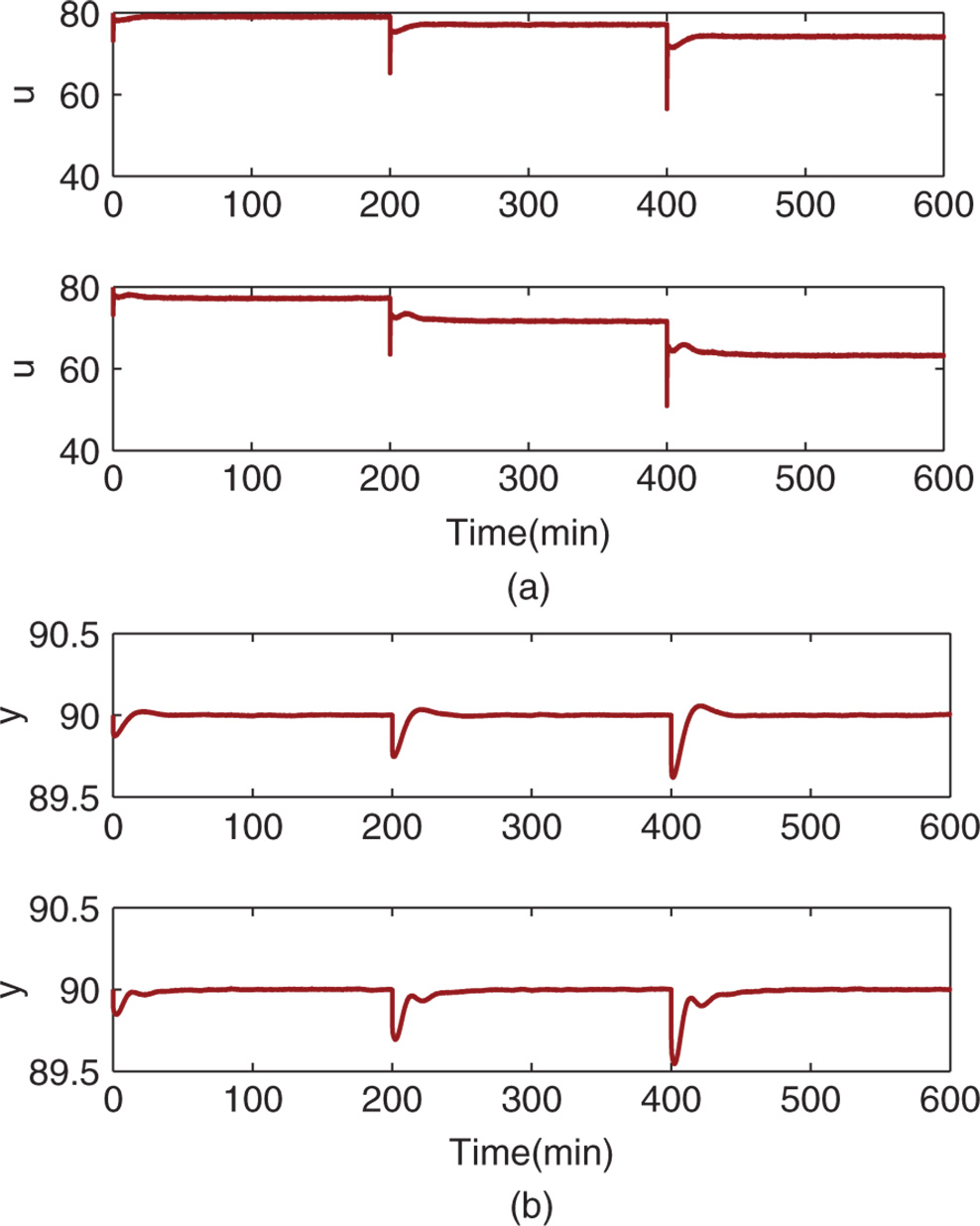
Figure 8.9 Closed-loop control simulation for output stair case disturbance rejection. (a) Control response (top figure: results from using  , bottom figure: results from using
  ). (b) Output response (top figure: results from using
  , bottom figure: results from using
  ).
).
8.3.6 Food for Thought
- In the PID controller parameter solutions (see (8.14)–(8.16)), is it correct to say that the proportional controller gain
 only uses the information from the first frequency point
  , however,
  and
and  use the information from both first and second frequency points?
 - Upon finding the controller parameters,
 ,
,  and
and  , using the information from the two frequency points, we have the options to test different combinations of controllers without changing their parameters. First instance, we can use the proportional controller with
  , PI controller with
  and
and  , PID controller with
  ,
,  and
and  or PD controller with
  and
and  . Why do you think that the frequency domain design can lead to such a result?
 - We have chosen
 and
and  for easy implementation. Can we choose other frequency points as
  and
and  as long as they are in the medium frequency range with cross-over frequency contained? Why is that?
 - In the specification of desired closed-loop transfer function (see 8.19), if the parameter
 , the closed-loop dominant time constant is specified to be equal to the open-loop dominant time constant but with unity steady-state gain. Would you consider this as a default choice?
8.4 PID Controller Design for Integrating Systems
PID control of integrating systems has become increasingly important in control engineering applications. A large number of electro-mechanical systems can be classified as integrating plus time delay systems. For instance, the angular position control of a robot is the control of integrating system, and the quadrotor control is also related to control of integrating systems.
The most widely encountered integrating systems have time delay in addition to first order or higher order dynamics. Because the integral action is expressed as a pole on the origin of the complex plane, which essentially is the dominant dynamics for an integrating system, it may not be necessarily to capture the first order or higher dynamics in the design of PID controllers. Instead, these stable dynamics are approximated using an equivalent time delay to describe the effect of their phase lag in the PID control system design.
8.4.1 The Approximate Model
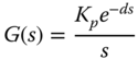
The approximate model of an integrating system is assumed to be of the following form:

where  is the gain of the integrating system and
  is its time delay. For most physical systems, there are more or less approximations involved in obtaining the integrating plus time delay model. An easy way to find the parameters in (8.22) is through frequency response analysis.
Assume that the frequency response  is available at the frequency
  . This frequency information
  is estimated using the relay experiments in many applications as shown in the next chapter.
Now, letting the frequency response of the integrating plus delay model (8.22) be equal to the measured  leads to
Equating the magnitudes on both side of (8.23) gives
where  . Additionally, from (8.23), the following relationship holds:

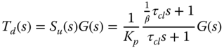
This gives the estimate of time delay as

It is seen here that if the system is truly integrating with time delay, the plant information at a single frequency is sufficient to determine the plant gain and time delay.
8.4.2 Selection of Desired Closed-loop Performance
Because the transfer function for the time-delay  is irrational, approximation is often needed when using the model based designs (see Chapter 3). An effective way to avoid the approximation is to derive the PID controller parameters using the frequency response analysis.
Similar to the PID controller design introduced in the previous section, we will first introduce the specification of desired closed-loop performance. Considering the PID controller structure

together with the integrating plus delay model
it is clear that the loop transfer function

contains a double integrator. Therefore, this characteristic should be reflected in the selection of the desired closed-loop performance. Additionally, the four characteristics of the desired complementary sensitivity function specified in Section 8.3.2 should be satisfied. It is simpler to choose the desired control sensitivity function to this effect.
A candidate for such a choice is the control sensitivity to have the following form:

where  is the desired closed-loop time constant and
  is the damping coefficient typically chosen as 0.707 or 1. A larger
  corresponds to a slower closed-loop response speed.
The desired complementary sensitivity function  is composed of the control sensitivity
  and the model
  given by

where the steady-state gain  and the factor
  have been cancelled to obtain (8.27).
It is seen from (8.27) that the desired complementary sensitivity function  has all poles on the left-hand side of the complex plane. Additionally, the complementary sensitivity
  is equal to unity at
  and the plant time-delay
  appears in the numerator of
  . Therefore, all the characteristic requirements discussed in Section 8.3.2 are satisfied for the integrating with time delay system by PID control.
Furthermore, a stable zero at  is introduced in the desired complementary sensitivity. The introduction of this stable zero is to ensure that at
  the desired loop transfer function
  will have the structure of a double integrator, which matches that of the actual loop transfer function
  in (8.25). This claim can be verified through the following calculation:

Writing the irrational transfer function  in Taylor series expansion gives

where  denotes the higher order terms in the Taylor series. Then, the denominator of
  is expressed as

Since from (8.30) the higher order  contains a factor
  , then it is clearly seen that the denominator
  contains the factor
  .
.
It is emphasized that the choice of  given by (8.27) ensures the desired loop transfer function
  has the feature of a double integrator at
  matching that of the actual loop transfer function
  . This means that at the lower frequency region, the PID controller parameters will automatically lead to the low frequency requirement of the sensitivity functions. This choice of desired complementary sensitivity function reduces the errors in the frequency curve fitting for computation of the PID controller parameters.
8.4.3 Normalization of the Parameters and Empirical Rules
To normalize the process parameters for derivation of the PID controller parameters in empirical rules, the actual loop transfer function  from (8.25) is re-written as

where  ,
,  ,
,  and
and  . For convenience in computation, (8.31) is expressed as

where the parameters are defined as

Note that the loop transfer function  is free of the process gain
  and the time delay
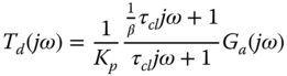
  . Similarly, the desired loop transfer function
  given by (8.28) is required to be normalized. To this end, the desired closed-loop time constant
  is selected as the function of the time delay
  :
:

where  is the desired closed-loop performance parameter used in the design. This leads to the re-writing of (8.28) in the following form:

Note that the desired loop transfer function  is also free of the time delay parameter
  .
.
The solution of the PID controller parameters follows from the frequency domain solution proposed in Section 8.3, but with different choices of the frequency points  and
and  (see Wang and Cluett (2000)).
Because the PID controller parameters are normalized, there are only the desired closed-loop time constant  and the damping coefficient adjustable. Thus, we can find the normalized PID controller parameters numerically with respect to the parameter
  and form empirical rules. There are two sets of empirical rules obtained below through polynomial fitting of the normalized PID controller parameters, together with gain and phase margins.
Selecting 100  values from
  to
to  with increment of 0.1, together with a damping coefficient
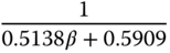
  , there are 100 sets of normalized PID controller parameters calculated. By using the polynomial fitting tool in MATLAB to find the calculated PID parameters, the following empirical rules for the normalized parameters are obtained as shown in Tables 8.1–8.2. With the normalized PID controller parameters calculated, the actual PID controller parameters are then obtained with the scaling parameters
  and
and  , as
, as

The polynomial functions in both Tables have provided quite accurate descriptions to the original data (see Figure 8.10 as an illustration). Therefore, when an integrator with delay is given, the PID controller parameters will be calculated simply using the polynomial equations presented in the tables.
Table 8.1 Normalized PID controller parameters ( ,
,  ).
).
 |
 |
 |
 |
 |
 |
Table 8.2 Normalized PID controller parameters ( ,
,  ).
).
 |
 |
 |
 |
 |
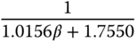 |
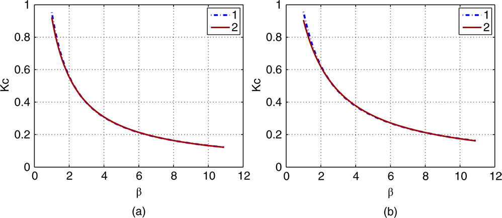
Figure 8.10 Calculated normalized proportional controller gain. (a)  ,
,  . (b)
. (b)  ,
,  . Key: line (1) data; line (2) using Tables 8.1 and 8.2.
8.4.4 Gain and Phase Margins
Because the original PID controller parameters are calculated using two frequency response data points, the PID controller parameters can be used in combination to obtain PID controller, PI controller and PD controller.
The gain and phase margins for the PID controllers are calculated using the empirical forms, which are also function of the parameter  and are shown in Figure 8.11. Additionally, the gain and phase margins for PI and PD controllers are calculated shown in Figures 8.12 and 8.13. These gain and phase margins are useful in measuring closed-loop performance and quantify robustness of the PID control system designed. It also provides some guidance on the choice of controller structures.
8.4.5 Simulation Examples
8.4.6 Food for Thought
- In the derivation of the PID controller rules for integrating with delay system, why is the desired closed-loop control sensitivity function specified with a stable zero?
- Do you expect an overshoot in closed-loop response to the step reference signal by observing the desired complementary sensitivity function
 in (8.27)? If you wish to eliminate such an overshoot, which reference filter should you choose in a two-degrees of freedom controller implementation?
 - To obtain an approximate integrating with time delay model, a frequency
 is required. Which region on the Nyquist curve of a system is a good candidate? Why?
8.5 Summary
This chapter has discussed several approaches to PID controller design using frequency domain information. PID controllers can be designed using gain margin and phase margin as their performance specifications in the frequency domain. One drawback with respect to the gain margin and phase margin specification is that these parameters are not related to the closed-loop response speed in a simple and intuitive way.
The other important aspects in the chapter are summarized as follows.
- PID controller parameters can be found analytically in a manner related to curve fitting of the open-loop frequency response in two frequency points. In this approach, the closed-loop performance specification is the desired dominant time constant via complementary sensitivity function.
- In order to produce the best fit possible with the limited number of controller parameters, the complementary sensitivity function contains the zeros of the plant as well as the time delay of the plant.
- A special case of the approach is the PID controller for integrator with delay system. With a normalized delay parameter, the PID controller parameters are simply expressed in empirical forms analytically with achieved gain margin and phase margin.
8.6 Further Reading
- The PID controller design methods using two points of frequency response data were originally introduced in Wang et al. (1995b), Wang and Cluett (1997b) and Wang and Cluett (2000).
- More PID controller design techniques using gain margin and phase margin specifications can be found in Ho et al. (1995), Ho et al. (1996), Ho and Xu (1998), Ho et al. (1998), Ho et al. (2000).
- Second order with delay model was obtained for PID controller design by using two frequency response points together with nonlinear optimization in Wang et al. (1999).
Problems
- 8.1 The transfer function of a complex system is given by
(8.37)

- Design a PI controller for this system by specifying the desired gain margin of
 .
. - Determine the phase margin and delay margin using Nyquist diagram.
- Design a PI controller for this system by specifying the desired gain margin of
- 8.2 The transfer function of a complex, underdamped system is given by
(8.38)

where
 .
.- Design a PI controller for this system by specifying the desired phase margin of
 .
. - Determine the gain margin and delay margin using Nyquist diagram.
- Show using simulation studies that the closed-loop response to a step input disturbance is oscillatory no matter what you do.
- Explain your results by examining the sensitivity function between the step input disturbance and output.
- Design a PI controller for this system by specifying the desired phase margin of
- 8.3 The mathematical model for the eighth reactor in a copolymerization reactor train is described by the following transfer function model (Madhuranthakam and Penlidis (2016)):
(8.39)

where the input is the flow rate of the Chain Transfer Agent (CTA) to the first reactor in the reactor train and the output is the weight-based average molecular weight (
 ). The parameters in the transfer function for the reactor are given as
  ,
,  and
and  . Design PID controller for this polymer reactor using two frequency response points (see Section 8.3).
- Choosing
 , which is case that the desired closed-loop transfer function equal to the open-loop transfer function, find the PID controller parameters.
 - Choosing
 and
and  , find the PID controller parameters.
 - Choosing
 and
and  , find the PID controller parameters.
 - Compare the Nyquist plots for the PID control systems and find their gain margin, phase margin and delay margin.
- Simulate the closed-loop PID control systems with unit step reference signal and a unit step disturbance entering the systems at half of the simulation time. The sampling interval
 is 1 (
 ), and the simulation time is 3000 (
 ) because it is a very slow process. In the simulation, both proportional control and derivative control are implemented on the output only to reduce overshoot in the reference response. The derivative filter time constant is selected as
  . For the simulations studies, use the MATLAB real-time function PIDV.slx created in Tutorial 4.1.
 - What are the observations when we compare the three PID control systems? What are the observations when we compare the three PID control systems with the results obtained in Example 2.7?
- What are the reasons behind the closed-loop performance improvement when using the frequency domain based design technique for this particular system?
- Choosing