10
PID Control of Multi-rotor Unmanned Aerial Vehicles
10.1 Introduction
This chapter will present the PID control of multi-rotor unmanned aerial vehicles as case studies. Because of nonlinearities and physical parameter uncertainties, the attitude control systems for an unmanned aerial vehicle are proposed to be PID control systems in a cascade structure and the PID controller parameters are found using the auto-tuners designed in Chapter 9. The auto-tuners are implemented on laboratory test rigs specifically designed for multi-rotor unmanned aerial vehicles and operated on the ground for the safety of the equipment. Experiments are conducted to evaluate the attitude control systems.
10.2 Multi-rotor Dynamics
This section will discuss the dynamics of a quadrotor and a hexacopter for the PID control system design. We will pay attention to their shared common features and their differences.
To ensure stable flight of a multi-rotor unmanned aerial vehicle (UAV), its attitude is required to be under feedback control. The attitude of a multi-rotor is captured by the variations of the three Euler angles: roll angle  , pitch angle
  and yaw angle
  . More specifically, the roll angle
  defines the rotation about the
  body axis, the pitch angle
  about the
  body axis, and the yaw angle about the
  body axis. To maintain stable flight with a multi-rotor UAV, the three Euler angles are required to follow desired reference signals in closed-loop control. The attitude control forms the common ground of PID control methodologies for multi-rotor UAVs. However, the difference comes from the details of the control signal realizations through actuators that are the rotors associated with the UAVs.
10.2.1 Dynamic Models for Attitude Control
From the control system design point of view, the outputs of an attitude control system are clearly the three Euler angles: roll angle  , pitch angle
  and yaw angle
  . One important reason why these three angles are selected as the outputs is that the reference signals to the angles are readily available. For instance, in order to maintain stable flight, the reference signals to the roll angle
  and pitch angle
  are commonly selected to be zero whilst the yaw angle
  is determined by the position of the UAV in the horizontal plane. The questions remain as what the control input signals are and how they are related to the output signals for the attitude control problem.
In order to derive the dynamic models for attitude control, a reference frame is defined. The mathematical models for the multi-rotor unmanned aerial vehicles share the same reference frame leading to the same dynamic models at this common ground. As an example, we examine the derivation of the dynamic models for a quadrotor UAV.
Figure 10.1 shows the framework used to derive a quadrotor dynamics model (Bouabdallah et al. (2004), Corke (2011), Derafa et al. (2006)), which illustrates that the origin of the body frame is in the mass center of the quadrotor UAV and the  -axis is upwards.
  , and
, and  are the four rotors and
  , and
, and  represent the rotors' angular velocities.
In order to obtain an unique solution for the mathematical models, the transformation sequence is assumed to be  . The input signals for the quadrotor are the torques
  ,
,  , and
, and  in the
  -,
-,  -, and
  -axes, respectively. In the same three dimensional space, we define
  ,
,  , and
, and  as their angular velocities and
  ,
,  , and
, and  as the moments of inertia for the three axes in the
  ,
,  , and
, and  directions. The quadrotor UAV is assumed to have a symmetric structure with four arms aligned with the
  -axis and
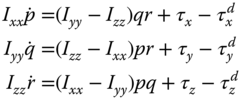
  -axis, and as a result there is no interaction between the torques along the three axes. From Euler's equation of motion (Bouabdallah et al. (2004), Corke (2011), Derafa et al. (2006)), the following dynamic equations in the
  ,
,  , and
, and  axes are obtained:

From the control system design point of view, if the multi-rotor UAV carries a payload, the load torque can be projected onto the  -,
-,  - and
- and  -axes, denoted by
  ,
,  and
and  . These quantities are unknown in general, and are considered as constant disturbances in control system design. With the consideration of load disturbances, we modify the motion equations as
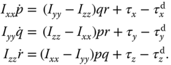
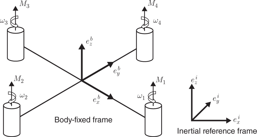
Figure 10.1 Inertial frame and body frame of the quadrotor.
If the payload is aligned with the mass center and is symmetric, the projections of the load torque on the  - and
- and  -axes are small.
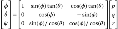
Now, the relationships between Euler angular velocities and the body frame angular velocities ( ,
,  , and
, and  ) are described in the following differential equations (Corke (2011)):

The dynamic models (10.2) and (10.3) present mathematical descriptions for the attitude control system design for the quadrotor. Clearly, there are three outputs in the control system, and the manipulated variables or the control signals are the three torques,  ,
,  , and
, and  , along the
  ,
,  , and
, and  directions.
The dynamic models for attitude control of a hexacopter are also described by the differential equations 10.2 and (10.3). Because a hexacopter uses six rotors attached to the end of each arm with equal distance from the vehicle's center of gravity, which is illustrated in Figure 10.2, it has better fault-tolerant properties and capability of carrying a larger payload than the quadrotor UAVs.
10.2.2 Actuator Dynamics for Quadrotor UAVs
It is worthwhile emphasizing that the dynamic models (10.1)–(10.3) derived for the quadrotor have not taken the actuators into consideration. The control signals, the torques  ,
,  , and
, and  in the body frame, will be implemented using DC motors. Thus, there will be additional first order or second order models used to capture the DC motor dynamics for the control system design.
In quadrotor control, the torques  ,
,  , and
, and  in the body frame are generated by the differences in rotor thrusts. The upward thrust produced by each rotor is
The total thrust is, hence,


Figure 10.2 Representation of a hexacopter (Ligthart et al. (2017)).
where  is the thrust constant determined by air density, the length of the blade, and the blade radius, and
  is the
  th rotor's angular speed.
When we only consider the attitude control, the altitude of the quadrotor UAV is not controlled and the total thrust  is manually set by the operator. Therefore, there will be an independent reference signal to the total thrust
  .
.
The torques about quadrotor's  -axis and
  -axis are


where  is the distance from the motor to the mass center. The torque applied to each propeller by the motor is opposed by aerodynamic drag, and the total reaction torque about the
  -axis is

where  is a drag constant determined by the same factors as
  .
.
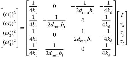
To determine the angular velocities for the four DC motors with regard to the control signals  ,
,  ,
,  , and
, and  , the linear equations 10.4–(10.7) are solved to give the following algebraic equations in the matrix form:
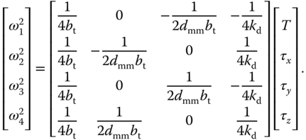
From (10.8), once the manipulated variables  ,
,  ,
,  , and
, and  are decided by the feedback controllers, the squared velocities,
  ,
,  ,
,  , and
, and  , of the motors will be uniquely determined.
From the context of feedback control, the squared velocities are translated into the velocity reference signals  ,
,  ,
,  , and
, and  that will be implemented in a typical DC motor drive, which are equal to the square roots of the components calculated using (10.8).
The DC motor dynamics will affect the closed-loop control performance, which should be included in the quadrotor model and they are approximated by a first-order transfer function:
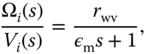
where  is the Laplace transform of the armature voltage
  to the
  th motor,
  is the Laplace transform of the motor velocity,
  is the time constant, and
  is the steady-state gain for the motor. The armature voltage
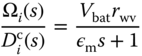
  is changed by manipulating the duty cycle of the pulse width modulation (PWM) signal of each motor drive, where the relationship between the motor armature voltage and the PWM duty cycle is

where  is the PWM signal duty cycle of the
  th DC motor drive and
  is the battery voltage assumed to be constant. Substituting equation 10.10 into equation 10.9 yields:
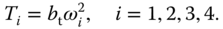
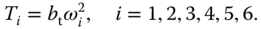
which describes the  th DC motor dynamics. To achieve the desired speed
  without steady-state error, a PI controller is required, which is designed by following the pole-assignment PI controller design method introduced in Chapter 3 with the parameters
  ,
,  and
and  . If we select two identical closed-loop poles at
  , then the closed-loop control system for the
  th DC motor is approximately a second order system with unit gain with the transfer function:
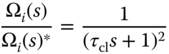
where  is the Laplace transform of the velocity reference signal to the DC motor. Because the DC motor control system has a very small time constant, the transfer function (10.12) is approximated using a time delay
  with the parameter
  determined through actual experiments.
The DC motor control systems are most commonly purchased together with the motors. Thus, for the implementation of the quadrotor control system, the control signals are the desired speed reference signals,  ,
,  ,
,  , and
, and  to the DC motors and their closed-loop dynamics are modeled by time delay components assuming the PI controllers are used in DC motor control.
10.2.3 Actuator Dynamics of Hexacopters
Similar to quadrotor control, the torques  ,
,  , and
, and  in the body frame of a hexacopter are generated by the rotor thrusts. The upward thrust produced by each rotor is
The total upward thrust is used to control the translational motion along the  -axis and is defined as follows:

where  is the thrust constant determined by air density, the length of the blade, and the blade radius, and
  is the
  th rotor's angular speed.
Let  be the distance from the center of gravity to the rotor and
  be the drag constant. For the hexacopter, the roll, pitch, and yaw control objectives are achieved by controlling the difference in thrust generated by each rotor, which is defined as:


Equations 10.13, (10.14), (10.15), and (10.16) can be arranged in matrix form as:
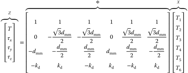
which has the simplified expression:

To implement the attitude control system, we need to determine the values of upward thrust  ,
,  . Unlike the quadrotor control case, from (10.17), there is no explicit one-to-one relationship between the actuators and the
  ,
,  ,
,  , and
, and  variables.
In the literature, this was often determined using the pseudo inverse of the matrix  , leading to

where  denotes the pseudo inverse of matrix
  .
.
An interesting approach is to borrow the idea from the model predictive control of hexacopter (Ligthart et al. (2017)) to formulate the inversion problem in terms of optimization. We define the following objective function:

where  denotes the transpose of
  matrix,
  is a positive definite matrix and for most cases, it is selected as a diagonal matrix with all positive elements. The first term in the objective function says that we would like to find the best
  vector such that the vector
  is matched as close as possible while the second term indicates that we wish the upward thrust vector to be limited with a weighting matrix
  . In most cases, we wish all the upward thrusts to have the same consideration, and
  is chosen as
  ,
,  , where
  is a diagonal matrix with dimension
  .
.
The minimization of objective function (10.19) leads to the following analytical solution:
Now, the matrix  is invertible because of the existence of the weighting matrix
  , which is positive definite.
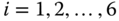
From the  , the six upward thrust values
  ,
,  are determined as well as the angular velocities of the six DC motors

These ωi values,  , will be used as reference signals
  for the motor control systems.
10.2.4 Food for Thought
- Which variables are used to define the attitude of a multi-rotor UAV?
- Neglecting the actuator dynamics, what are the input and output variables for the attitude control of a multi-rotor UAV? Taking the actuators into consideration, what are the input and output variables?
- For the DC motor control problem, if the battery voltage is less than expected, will the motor drive increase or decrease the duty cycle to compensate the discrepancy?
- From the mathematical modelling, do you think that it is important to use a PI controller to control the velocity of each motor?
- Which constants do you need to determine in order to implement the control system? Which constants do you need to determine for the attitude control system design?
- Are there any redundancies in the actuators for the hexacopter?
10.3 Cascade Attitude Control of Multi-rotor UAVs
In order to fly a UAV, the closed-loop control of the three Euler angles  ,
,  , and
, and  is necessary. Because of the products of angular velocities in (10.2) and the sinusoidal functions in (10.3), a multi-rotor UAV is a nonlinear system.
In theory, combining (10.2) with (10.3) will lead to three second order nonlinear systems. Therefore, three PID controllers could be adequate for the attitude control applications. However, in practice, a cascade PI or PID controller structure offers a better solution for the following reasons.
- If the multi-rotor UAV carries a payload [see (10.2)], the load disturbance is much more effectively rejected in a cascade control system structure because it occurs at the secondary plant [see Chapter 7].
- Looking at Euler's equations of motion (10.1), if the multi-rotor UAV is well designed with a balanced load, the moment of inertia at the
 -axis and
  -axis equal each other:
  . However,
  in general. There are interactions between the variables
  and
and  . The interactions in a PID controlled system would be translated as disturbances. We could compensate their effects using a feedforward control action as shown in Section 3.6 if the parameters
  ,
,  , and
, and  are available with reasonable accuracy. Alternatively, we simply neglect them in the PID controller design, and they are automatically compensated in the feedback control using a high gain feedback control. Clearly the bilinear terms in (10.1) act on the torques
  ,
,  , and
, and  , and they are regarded as input disturbances to the multi-rotor UAV system. It was shown in Section 7.3 that the cascade control system has a much improved performance in disturbance rejection. The existence of bilinear terms in (10.1) is one consideration for the choice of cascade control system.
 - Because the torques
 ,
,  , and
, and  will be realized by the electrical motors installed on the multi-rotor UAV and the motor dynamics are not captured in the motion equations, there will be model uncertainties in the mathematical models having an impact on the closed-loop control. These uncertainties occurring in the secondary plant are better dealt with in a cascade control structure.
 - Above all, the cascade control structure offers a simpler controller design framework because for each stage only first order models or first order plus time delay models are involved.

Figure 10.3 Attitude control system structure.
Figure 10.3 shows the cascade control system configuration for the attitude control of a multi-rotor UAV where the body frame angular velocities  ,
,  , and
, and  along the
  ,
,  , and
, and  directions are the secondary variables. With this configuration, the secondary system is described by the differential equations given in (10.1), and the primary system is described by (10.3). To control the angular velocities of the multi-rotor UAV, three PI controllers are used to calculate the control signals based on their respective reference signals
  , and
, and  . Additionally, there are two PI controllers to control the roll and pitch angles, where their reference signals are
  and
and  .
.
10.3.1 Linearized Model for the Secondary Plant
The dynamic models in (10.1) used for the design of secondary controllers are expressed as

where the load disturbances are neglected. Clearly, the secondary plant is integrating systems with gain inversely proportional to their moment of inertia constant.
If one wishes to use feedforward compensation as in Section 3.6 of Chapter 3, the intermediate variables are defined as

With these variables defined, the dynamic models (10.21) for the secondary plant become:

The dynamics from actuators, i.e. the rotors, can be modeled as a time delay  with a gain
  because their time constants are relatively small in comparison with the dynamics from the secondary plant. In short, the secondary plant in the multi-rotor UAV system is approximated by three integrator with time delay models.
10.3.2 Linearized Model for the Primary Plant
For the problem of attitude control, the nonlinear plant for the three Euler angles is required to be linearized around their operating conditions. To maintain stable flight, the reference signals to the roll and pitch angles ( and
and  ) are chosen to be zero at the steady-state operating conditions while the reference signal to the yaw angle
  may change according the position reference signals of the multi-rotor UAV. Thus, the linearization of the nonlinear equations 10.3 at the steady-state operating conditions (
 ) gives:

With consideration of time delay from the secondary closed-loop system, the primary plant is approximately modeled using an integrator with the time delay model.
Depending on a time delay existing in the system, one may wish to use PID controllers for the secondary or primary plant if closed-loop control performance can be improved with the derivative action.
10.3.3 Food for Thought
- In the cascade control structure, what are the reference signals for
 and
and  to ensure a stable flight?
 - How do we generate a reference signal for yaw rate
 if the position of a multi-rotor UAV is controlled by an operator?
 - Do we need the total thrust
 in the cascade attitude control system?
 - Is it correct to say that we can not change
 ,
,  and
and  directly although they are the manipulated variables? If it is correct, which variables can be changed that will result in the changes in
  ,
,  and
and  ?
? - Is it correct to say that the dynamic models for the secondary plant are not accurate because the actuators are not considered?
- With the cascade control structure, we still face the choice of P, PI, or PID controllers for each loop. Which factors and criteria do you consider for the selection of the controller structures for each individual loop?
10.4 Automatic Tuning of Attitude Control Systems
The dynamic models for the attitude control system are relatively simple with the parameters from the moments of inertia,  ,
,  , and
, and  . However, the parameters associated with the actuators are more complicated if one wishes to measure them accurately. The purpose of using an auto-tuner for the attitude control system is to avoid the time consuming tasks of finding the physical parameters for the secondary and primary plants as well as the actuators. In addition, the dynamics of the closed-loop secondary system are taken into consideration in the primary control system through the application of the cascade auto-tuner.
In order to implement the cascade PI control system with auto-tuner for a multi-rotor UAV, the coefficients  ,
,  and
and  are pre-determined so that the reference signals to the rotors in the example of quadrotor UAV are calculated using the equation below:
where  ,
,  ,
,  , and
, and  are the attitude controller outputs, which are used to generate the desired velocities for the rotors. For a DC motor with a commercial drive, a PI controller is often used for controlling its velocity where the desired the velocity reference signal
  ,
,  , is used for each motor.
A similar approach is adopted for the hexacopter by calculating the desired rotor velocities using (10.18).
The auto-tuning algorithms for an integrator with delay systems were developed in Section 9.7. They are used for tuning both primary and secondary controllers in the multi-rotor UAV applications without modifications. More detailed discussions on auto-tuning of attitude control for multi-rotor UAVs can be found in Chen and Wang (2017) and Poksawat and Wang (2017).
10.4.1 Test Rigs for Auto-tuning Cascade PI Controllers of Multi-rotor UAVs
In order to conduct identification experiments in a controlled environment, the quadrotor is fixed on a mechanical stance for the testing on ground in order to ensure safety of the electronics during the testing process. The test rig is shown in Figure 10.4, which was built and used to conduct the relay experiments for identification of the quadrotor's two-axis dynamics. For instance, with the objective to identify the integrator with a delay model for the roll angle, two quadrotor arms along the  -axis are fixed on the stand and the quadrotor can only rotate about the
  -axis. Furthermore, the test rig is carefully adjusted to make rotating axis aligned with the quadrotor's body frame axis, so that the torque due to weight force is minimized. As the quadrotor platform is very light and the two rotating pivots are very smooth, the friction is negligible in the experiments.
A similar test rig is also built for the hexacopter as shown in Figure 10.5.
10.4.2 Experimental Results for Quadrotor UAV
The quadrotor consists of five main components: RC transmitter/receiver, IMU sensor board, data logger, microprocessor, and actuators. The RC transmitter/receiver is to send and receive reference signals. The IMU sensor board is to measure the Euler angles and angular velocities. The data logger is to record flight data such as Euler angles and reference signals. The micro-processor is to generate control signals to stabilize the UAV's attitude. The actuators are to generate thrust and torques, which consist of motor drives, DC motors, gearboxes, and blades. The quadrotor's hardware used in the experimental tests is listed in Table 10.1.

Figure 10.4 Quadrotor test-bed.

Figure 10.5 Experimental rig for a hexacopter.
Table 10.1 Quadrotor hardware list.
| Function | Model |
| DC motor drive | DRV8833 Dual Motor Driver Carrier |
| Sensor board | MPU6050 |
| Micro processor | STM32F103C8T6 |
| RC receiver | WFLY065 |
| DC motor | 820 Coreless Motor |
| RC transmitter | WFT06X-A |
| Data logger | SparkFun OpenLog |
The sampling interval  for the secondary, primary controllers and relay test are all set to be 0.01 s, which is the IMU sensor's maximum updating rate. The other physical parameters of the quadrotor are shown in Table 10.2.
The auto-tuning of the cascade PI control system begins at the inner loop. Before the relay control experiment, a proportional controller  is selected to stabilize the secondary system. The sensor measurement of velocity,
  , contains noise. Thus, a relay amplitude of 0.8 together with a hysteresis level of 0.1 is selected to reflect the measurement noise level. Figure 10.6 shows a segment of the relay feedback control data. From the input signal to the inner-loop, closed-loop control system, the period of the sustained oscillations is identified as
  samples, leading to the fundamental frequency in the frequency sampling filter as
  (rad). The use of the frequency sampling filter based estimation algorithm gives the inner-loop, closed-loop frequency response as
Table 10.2 Quadrotor parameters.
| Parameters | Description | Value | Unit |
 |
Moment of inertia about  axis axis |
 |
kg  |
 |
Moment of inertia about  axis axis |
 |
kg  |
 |
Moment of inertia about  axis axis |
 |
kg  |
 |
Thrust constant |  |
N/A |
 |
Drag constant |  |
N/A |
 |
Quadrotor total mass | 0.145 | kg |
 |
Motor to mass center distance | 0.110 | m |
 |
Battery voltage | 8.28 | V |
 |
Motor's DC gain | 137.6571 | rad   |
 |
Rotor normal speed | 606.2469 | rad  |
 |
Motor delay | 0.032 | s |
 |
Motor time constant | 0.072 | s |

Figure 10.6 Relay feedback control signals from the inner-loop system: top figure, input signal; bottom figure, output signal.

Converting this discrete-time frequency to continuous time frequency, which is  (rad
(rad  ), together with the knowledge of the proportional controller used in the relay experiment (
 ), the continuous-time frequency response of the inner-loop plant is calculated as

From this frequency information, an integrator plus delay model is identified as

By choosing the desired closed-loop time constant as three times the estimated delay:  (s) and damping coefficient of 1, from the empirical rules shown in Section 8.4.3, the PI controller parameters are found for the inner-loop control system as
  and
and  . This set of PI controller parameters approximately gives a gain margin of 3 and phase margin of
  for the closed-loop system with the integrator plus delay model.
Figure 10.7 shows the closed-loop step response of  where the reference signal has a magnitude of 0.5 (rad
  ). It is seen from this figure that the closed-loop velocity response follows the reference signal without steady-state error, and there is a large overshoot and a slight oscillation. Additionally, there are disturbances and measurement noise in the inner-loop system. For a cascade control system, the inner-loop control system is required to have a fast response speed, which is achieved in the design here.
The second step in auto-tuning the cascade control system is to find the outer-loop controller. For the outer-loop experiment, the proportional controller  is used to stabilize the integrator with delay system. The amplitude of the relay is selected to be 0.4 and the hysteresis level
  is 0.05 to prevent the relay from random switching. Figure 10.8 shows a segment of the input and output data generated from this relay feedback control of the primary plant under proportional control. The averaged period of the sustained oscillation is
  in number of samples, which gives the fundamental frequency in discrete time as
  (rad). A frequency sampling filter model is used to estimate the closed-loop frequency response based on the set of input and output data shown in Figure 10.8, yielding to

Figure 10.7 Inner-loop step response in closed-loop control. Dashed line, reference signal; solid line, output.

Figure 10.8 Relay feedback control signals from outer-loop system: top figure, input signal; bottom figure, output signal.

With the proportional controller  , the frequency response of the outer-loop system is found at
  (rad
(rad  ) as
) as

From this frequency information, the integrator plus delay model for the primary system is calculated as

For a typical cascade control system design, the outer-loop control system should have a slower desired closed-loop response than that of the inner-loop control system. By selecting the desired closed-loop time constant as eight times the delay value: 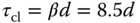 with damping coefficient
  which gives gain margin
  , and phase margin
  (see Section 8.4.3, the PI controller parameters are calculated using the empirical rules:

For comparison purposes, with a faster desired closed-loop time constant  and a slower desired closed-loop time constant
  , two additional sets of PI controller parameters are calculated as
  ,
,  , and
, and 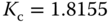 ,
,  .
.
Figure 10.9 shows the comparative closed-loop responses for the three cases experimentally. It is seen from the comparative results that all three PI controllers lead to stable closed-loop systems. Clearly when  , the fastest closed-loop response is obtained. A sequence of step reference changes is applied to the roll angle for a further experimental test, as shown in Figure 10.10, which shows a fast response with an overshoot.

Figure 10.9 Comparative roll angle step response in closed-loop control.
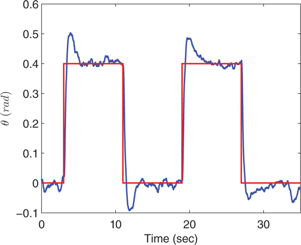
Figure 10.10 Roll angle step response of quadrotor using test rig.
We note that the estimated integrator with delay model for the roll angle given in (10.25) has a gain of 1.54, which is much larger than the expected value of 1 because the secondary closed-loop system should have unit gain under PI control. This could be caused by the existence of the nonlinearity or how the IMU sensor behaves when the roll angle swings with a large amplitude.
10.4.3 Experimental Results for Hexacopter
A hexacopter is built for experimental testing of the auto-tuner and the cascade attitude control system (Poksawat and Wang (2017)). The flight controller specifications and avionic components are presented in Table 10.3. The physical parameters are presented in Table 10.4.
To validate the proposed strategy, an automatic tuning experiment is performed on the hexacopter and the results are presented here. Firstly, the roll angular rate controller parameters are tuned with the relay test. It is assumed that the airframe is symmetrical, thus the pitch controller parameters are selected to be identical to those obtained in the experiments from the roll axis. For the yaw angular rate loop, the tuning procedure will follow the same approach. The sampling interval  is chosen to be 0.006 s.
Table 10.3 Flight controller and avionic components.
| Components | Descriptions |
| Airframe | Turnigy Talon Hexacopter |
| Microprocessor | ATMega2560 |
| Inertial measurement unit | MPU6050 |
| Electronic speed controllers | Turnigy 25A Speed Controller |
| Brushless DC motors | NTM Prop Drive 28-26 235W |
| Propellers | 10x4.5 SF Props |
| RC receiver | OrangeRX R815X 2.4Ghz receiver |
| RC transmitter | Turnigy 9XR PRO transmitter |
| Datalogger | CleanFlight Blackbox Datalogger |
Table 10.4 Physical specifications of the hexacopter.
| Parameters | Details |
Mass ( ) ) |
1.61 kg |
Arm length ( ) ) |
0.3125 m |
Blade radius ( ) ) |
0.127 m |
Moment of inertia ( ) ) |
0.2503 kg  |
Moment of inertia ( ) ) |
0.2914 kg  |
Moment of inertia ( ) ) |
0.6177 kg  |
Thrust constant ( ) ) |
 |
Torque constant ( ) ) |
0.0209 |
Figure 10.11 Inner loop relay test result.
For the automatic tuning of the secondary controller, which is the roll angular rate, the proportional gain used in the relay test is chosen as  for stabilization of the integral system. The amplitude of the relay reference signal has to be within the operating condition of the hexacopter UAV, thus it is selected as
 . The hysteresis is chosen to be
 to prevent the relay switching from measurement noise.
A section of the relay feedback experimental data is presented in Figure 10.11. The period of the sustained oscillations is calculated to be  , leading to the fundamental frequency in the sampling filter of
  rad.
rad.
The inner loop frequency response is then estimated using frequency sampling filter estimation algorithm as

The continuous time frequency can be calculated as  (rad
(rad  ). From this, the continuous time frequency response of the secondary plant is

The integrator plus time delay transfer function is obtained as

For the hexacopter, we decided to use a PID controller instead of a PI controller because the delay is quite large and the derivative term improves the closed-loop response. In order to achieve fast closed-loop system response, the desired closed-loop time constant is selected to be relatively small. Here,  is selected as 1, which leads to an approximate gain margin of 2 and phase margin of
  respectively. The controller parameters for the roll angle rate system are then obtained as
  , and
, and  from using the empirical rules presented in Section 8.4.3.
Once the inner loop controller is tuned, the outer loop controller's parameters can be selected with the following procedures. Instead of automatic tuning of the primary controller, the mathematical model for the primary plant is approximated by the following integrator with delay system:
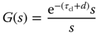

Figure 10.12 Attitude control system with approximated inner loop.
where the integrator is from the primary plant (roll angular rate to roll angle) and the time delay is from the approximation of the closed-loop secondary system, where  is the closed-loop time constant and
  is the time delay from the inner-loop. Figure 10.12 shows the primary control system.
Generally, for a control system with a cascaded loop configuration, the outer loop response time needs to be slower than the inner loop. Hence, the outer loop time constant is chosen to be twice of the time delay, leading to the controller parameters for the angular position loop as  , and
, and  .
.
An outdoor flight test was conducted to validate the stability of the UAV in real flight against external disturbances such as turbulence (see Figure 10.13). The roll, pitch, and yaw data obtained from the flight test are presented in Figures 10.14, 10.15, and 10.16 respectively. The dashed lines represent the reference signals and the solid lines represent the measured flight data.
It is clearly seen that the hexcopter is able to follow the pilot's commands, due to the fact that the outputs are regulated closely to their references. Furthermore, it is able to hover, roll, pitch, and yaw while maintaining stability.
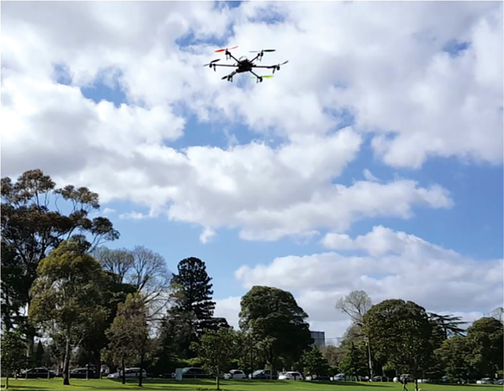
Figure 10.13 Outdoor flight test.

Figure 10.14 Flight data for roll axis.
Figure 10.15 Flight data for pitch axis.

Figure 10.16 Flight data for yaw axis.
10.4.4 Food for Thought
- What are the steps required to implement the auto-tuners?
- Is it correct to say that the relay experiments because they are conducted in closed-loop with a feedback controller
 , are relatively simple to implement using the existing cascade control structure of a multi-rotor UAV?
 - If the parameters
 ,
,  and
and  are not precisely measured, will the auto-tuner compensate the errors because of the experiments are carried out on the actual physical system?
 - Have the integrator with delay models for the secondary plant included the actuator dynamics?
- If an integrator is included in the controller for the secondary plant, what is the steady-state gain of the primary plant? What is the minimum value of the estimated time delay for the primary plant?
- Will PD controllers be adequate for controlling both secondary and primary plants of the multi-rotor UAV? What problems would you envisage that might occur?
10.5 Summary
We have discussed PID control of multi-rotor unmanned aerial vehicles in this chapter. Dynamic models for both quadrotor UAV and hexacopter UAV are discussed from the control system design point of view. Cascade control system structures are proposed for both quadrotor and hexacopter UAVs. The auto-tuning algorithms introduced in Chapter 9 are used to find the PID controller parameters for the UAVs on test rigs. The cascade PID control systems are experimentally evaluated through outdoor flight tests.
The other important aspects of the chapter are summarized as follows.
- Both inner-loop and outer-loop systems for the unmanned aerial vehicles are modelled using integrator with time delay systems.
- A proportional controller is used to produce a stable closed-loop system prior to the implementation of auto-tuner.
- Both PID controller and auto-tuner implementations on the UAVs have used micro-controllers. The programs for PID implementations have included anti-windup mechanisms and are based on Tutorial 4.1. The auto-tuner implementations are based on Tutorial 9.1 for the relay feedback control.
- The estimation of frequency response of the UAVs is performed based on Tutorial 9.4.
- Upon obtaining the estimation of the frequency response, we can follow the computational examples presented in Section 9.7 to calculate the PID controller parameters.
10.6 Further Reading
- Books for unmanned aerial vehicles include Beard and McLain (2012), Fahlstrom and Gleason (2012), Austin (2011) and Gundlach (2012).
- Mathematical modelling and control of hexacopter were presented in Alaimo et al. (2013). Detailed nonlinear modelling together with control was presented in Bangura and Mahony (2012). Nonlinear control of quadrotor UAV was presented in Goodarzi et al. (2013). A survey of control methods was presented in Li and Song (2012).
- Automatic tuning of the PID attitude control systems for the quadrotor UAV presented in this chapter was designed and experimentally validated in Chen and Wang (2016) and in Chen (2017). The closed-loop performance was assessed on ground using the same test rig based on system identification of the closed-loop transfer function (Chen and Wang (2015)). Automatic tuning of the PID attitude control systems for the hexacopter presented in this chapter was designed and experiementally validated in Poksawat and Wang (2017). Automatic tuning of PID attitude control systems for a micro fixed-wing UAV can be found in Poksawat et al. (2016), Poksawat et al. (2017) and Poksawat (2018).
- Optimization based tuning method was used to find controllers for an auto-pilot of fixed-wing UAV (Ahsan et al. (2013)).
- Model predictive control system was designed and experimentally validated for the hexacopter presented in this chapter (Ligthart et al. (2017)).
Problems
- 10.1 The dynamic models for a multi-rotor UAV without considering the actuator dynamics are described by the following differential equations (see (10.2)–(10.3)):
and
where the moments of inertial constants are
 (
( ),
),  (
( ) and
) and  (
( ).
).- Build a Simulink simulation model for the multi-rotor UAV without actuator dynamics.
- With zero initial conditions for all the state variables
 and
and  , compute the open-loop responses of the states to the load disturbances
  ,
,  and
and  . Here, we assume that the reference signals to the open-loop system are
  and the sampling interval is
  (sec).
 - What are your observations on the system dynamics from this open-loop simulation exercise?
- 10.2 Continue from Problem 10.1. Design a cascade PI control system for the multi-rotor UAV. The desired closed-loop poles for the secondary plant are all chosen to be
 and for the primary plant are all chosen to be
  . Use the model based PI controller design method in Chapter 3 to find the PI controller parameters.
- Choosing the reference signals
 and
and  , and simulate the cascade closed-loop control system's responses to the reference following and disturbance rejection. You may use a smaller sampling interval to improve the numerical stability in the simulation.
 - Increase the load torque
 to 0.4 and observe how the control signals
  ,
,  and
and  change in comparison to the responses from the original load of 0.2.
 - Vary the desired closed-loop poles for both secondary and primary control systems and observe the changes on the control signals
 ,
,  and
and  , and output signals
  .
.
- Choosing the reference signals
- 10.3 Continue from Problem 10.1. Instead of the cascade control structure, design three PID controllers using the linearized models from (10.26) and (10.27). For simplicity, we may choose all closed-loop poles at
 and tune the parameter
  to achieve closed-loop stability from the nonlinear control system simulation. The pole-assignment controller design introduced in Chapter 3 is used to find the parameters of the PID controller with filter.
- What are the
 values found to achieve closed-loop stability without oscillations?
 - What are your observations on the disturbance rejection when comparing this control system with the previous cascade control system?
- What are the
- 10.4 Modify the Simulink simulator built from Problem 10.1 to consider the actuator dynamics. For simplicity, the actuator dynamics for each axis are modeled using the delay model
 . Choosing
  second, through the nonlinear system simulation determine the range of
  for the closed-loop stability of the cascade control system.
 - 10.5 Using the physical parameters from Table 10.2, we build a Simulink simulation model for the quadrotor UAV with actuators. Perform automatic tuning of the PID controllers for the quadrotor using simulation studies. The closed-loop time constants for the secondary controllers are selected as
 where
where  is the estimated delay and for the primary controllers are selected as
  .
.