6
PID Control of Nonlinear Systems
6.1 Introduction
One of the approaches to obtain the models for the control system design is based on analysis of the system dynamics using first principles, such as mass balance, Newton's laws, current law and voltage law. The majority of these types of models are nonlinear in nature. Thus, in order to use them for the PID controller design or other linear time invariant controller design, these nonlinear models need to be linearized around the operating conditions of the system.
This chapter will introduce linearization of nonlinear models through several examples and case studies. It will also show how to apply the PID controllers to a nonlinear plant using the technique called gain scheduled control.
6.2 Linearization of the Nonlinear Model
The starting point of designing a PID controller for a nonlinear plant is to obtain a linear time invariant model through linearization around the chosen operating conditions of the system.
6.2.1 Approximation of a Nonlinear Function
Assume that the nonlinear models have the general form:
where  is a nonlinear function. The purpose of linearization is to find a linear function (a set of linear functions) to describe the dynamics of the nonlinear model at a given operating condition.
In order to understand how the linearization is performed, we first examine the case of linearization of a nonlinear function. It begins with a Taylor series expansion and approximation of a nonlinear function. As we know, a function with variable  ,
,  can be expressed in terms of a Taylor series expansion at
  , where
  is a constant, as

if the function  is smooth and its derivatives exist for all the orders. All the derivatives are evaluated at
  .
.
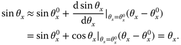
Using the first two terms in the Taylor series expansion leads to the approximation of the original function  at a specific point
  ,
,
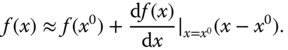
This first order Taylor series approximates the original nonlinear function  using the function evaluated at
  and its first derivative at
  . The approximation holds in the vicinity of
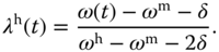
  . Figure 6.1 illustrates an example of a linear approximation of a nonlinear function where
  ,
, 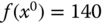 and
and 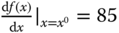 . It is seen that within the region where
  is close to
  ,
,  is closely approximated by the first order Taylor series expansion (6.3). Intuitively, we can think of the original variable
  as a “large” variable because it covers a large region, and the perturbed variable
  as a “small” variable because it covers a small region around
  .
.
If the nonlinear function  contains
  variables, meaning that
 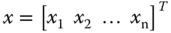 is a vector with dimension
  , then the function is approximated using the first
  terms in the multi-variable Taylor series expansion as
Note that we need the partial derivatives of the nonlinear function against all its variables. Similar to the single variable case, the multi-variable Taylor series expansion consists of the constant term that is the nonlinear function evaluated at  , followed by the partial derivatives with perturbations
  . Furthermore, the first order Taylor series expansion approximates well the original nonlinear function if the variables
  are in the vicinities of
  .
.
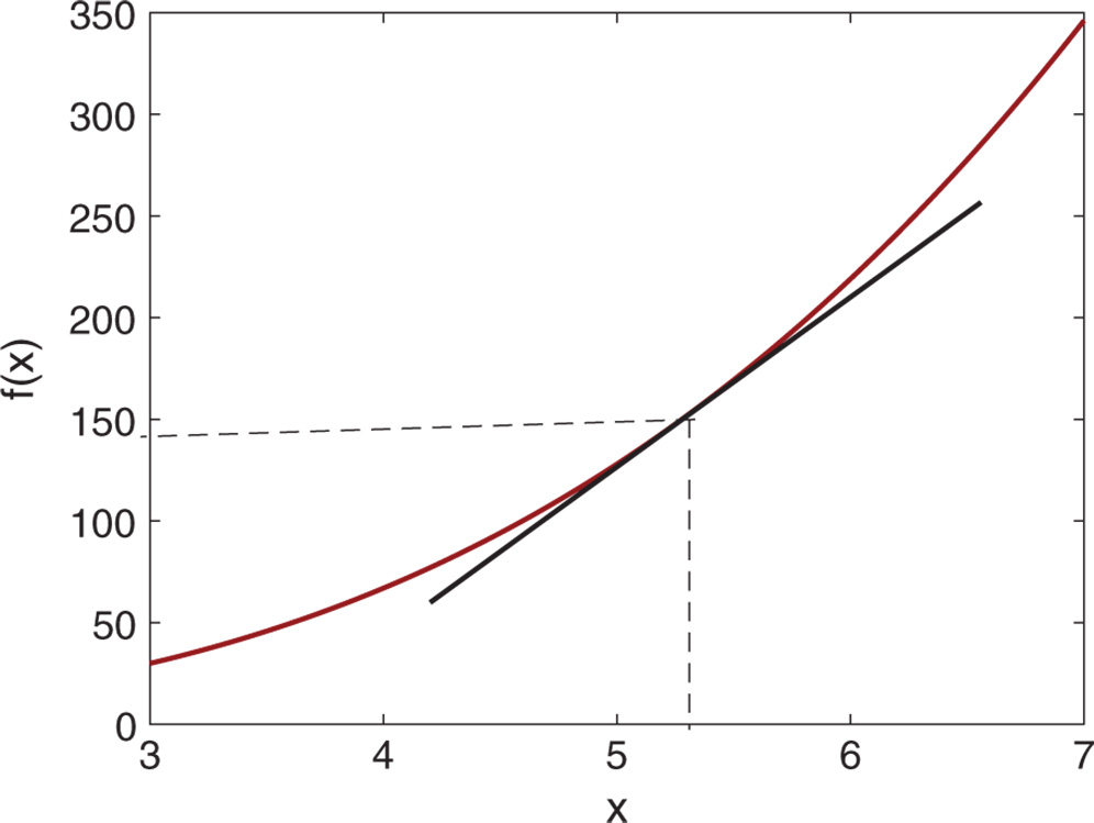
Figure 6.1 Approximation of a nonlinear function at  .
.
6.2.2 Linearization of nonlinear differential equations
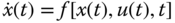
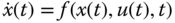
The nonlinear models obtained from using first principles of the physical laws are differential equations. We assume that the nonlinear differential equation used to describe a physical system takes the general form:
where  is a vector that represents the state variables of dimension
  and
and  is a vector for the control signals of dimension
  .
.
In linearization of a nonlinear dynamic system, we will firstly choose the constant vectors  and
and  , and apply the linearization procedure of the nonlinear functions as outlined in the previous section. We may write the final results in matrix and vector forms.
The constant vectors  and
and  play an important role in the linearized model. To make the linearized system truly linear, these vectors need to be selected carefully. The point of interest is called an equilibrium point for the nonlinear dynamic system (6.5), which was originated from nonlinear control (see Bay (1999)). These equilibrium points in control system design and implementation are often referred to as stationary points, which represent a steady-state solution to the dynamic equation 6.5. In general terms, an equilibrium point is defined by a constant vector
  such that if
  ,
,  , then
  .
.
Since an equilibrium point is a constant vector, the nonlinear differential equation 6.5 satisfies the following relationship:
The concept of equilibrium points is extended to constant vectors  and
and  such that the following steady-state solution of the nonlinear differential equation 6.5 is true:
These constant vectors are not dependent on time; however, they are allowed to vary as desired trajectories. In fact, they correspond to the steady-state values of the system that have been discussed previously in the PID control system implementation (see Chapter 4).
In control applications, it is often to choose the desired values for the state variables  , and solve the nonlinear algebraic equation given by (6.7) to determine the constant vector
  . However, because of the uncertainty associated with the physical parameters and unknown disturbances, the characterization of the operating conditions of the system by the pair
  and
and  could be quite inaccurate and far from reality.
The shortcoming caused by the inaccuracy of steady-state parameters can be overcome by the action of an integrator contained in the controller as the discrepancy is modeled as a constant input disturbance to the system. The integral action will automatically adjust the steady-state value of the input signal to achieve zero steady-state error in the output signal.
6.2.3 Case Study: Linearization of the Coupled Tank Model
Two cubic water tanks are connected in series as illustrated in Figure 6.2. Water flows into the first tank and flows out from the second tank. A pump controls the water in-flow rate  (
( ) to the first tank; and another pump controls the water out-flow rate
  (
(
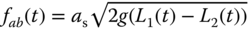
 ) from the second tank. Water flows from tank A to tank B, with a flow rate
  . The unit for the flow rate is
 and the unit for the water level is m.

Figure 6.2 Schematic of a double tank.
Using mass balance, the rate of change of water volume  in tank A is
The water volume can also be expressed as  , where
  is the cross-sectional area of the tank A, and
  is the water level in tank A. The dynamic equation to describe the rate of change in the water level
  (tank A) is
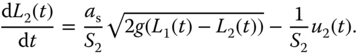
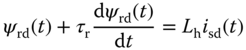
Likewise, the rate of change in the water level  is
is

where  is the cross-sectional area for tank B. For a small orifice with a cross-sectional area
  (
( ),
),  is linked to the tank levels
  and
and  by the following relationship:
where  is acceleration due to gravity (
 m
m  );
);  is the flow rate (
 ).
).
By substituting (6.11) into (6.9) and (6.10), we obtain

Both of these models are nonlinear.
6.2.4 Case Study: Linearization of the Induction Motor Model
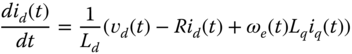
From the literature, several standard models of induction motor are available to use for control system design (Quang and Dittrich (2008), Wang et al. (2015)). Among them is a mathematical model with four differential equations in direct-quadrature (dq) coordination, which is originated from the field oriented control theory (Quang and Dittrich (2008), Wang et al. (2015)). When the parasitic effect such as eddy currents, magnetic field saturation are neglected, the dynamic model of an induction motor is governed by the following differential equations (Wang et al. (2015)):

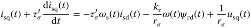
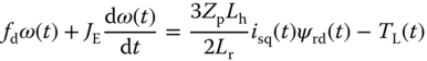

where  and
and  are the stator currents in the dq coordination,
  is the rotor flux in the d-axis and the input variables
  and
and  represent the stator voltages in the dq coordination.
  and
and  are the synchronous and rotor velocity respectively.
  is the load torque that might change with respect to time. The rest of the parameters are physical parameters with descriptions in Wang et al. (2015). For example,
  and
and  are the stator resistance and inductance,
  and
and  are the rotor resistance and inductance,
  is the mutual machine inductance;
  is the friction coefficient,
  is the inertia constant and
  is the number of pole pairs. The manipulated variables in the induction motor control problem are the stator voltages,
  and
and  , and the output variables are the rotor velocity
  and the rotor flux in the d-axis,
  .
.
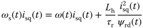
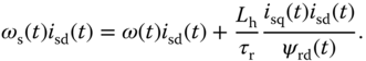
In the above model, there are four bilinear terms contained in (6.21)–(6.24). However, because the synchronous velocity  is not a state variable, it needs to be replaced by the slip equation 6.25, which leads to the following nonlinear terms:
By pre-defining operating conditions and the steady-state parameters,  ,
,  ,
,  ,
,  ,
,  , the nonlinear terms are approximated using a first order Taylor series expansion around the steady-state parameters. In particular, the following approximations are used in the derivation of the linearized model,


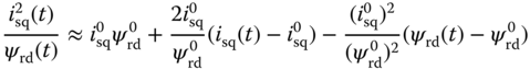

Although the variables  ,
,  ,
,  ,
,  are the actual physical variables, not the deviation variables, the approximation relations are only valid in the vicinity of the steady-state conditions as they are based on a Taylor series expansion. From (6.28)–(6.33), it is seen that information about the steady-state values of
  ,
,  ,
,  , and
, and  is required to obtain the parameters for the linearized terms. Since the output variables are
  and
and  , the steady-state parameters for these variables will be chosen to be equal to their desired reference signals. In particular, in the application of induction motor control, the reference signal to rotor flux is often fixed as a constant with its value dependent on the operating speed and load condition of the induction motor. For instance, the reference signal for
  is recommended to be 0.35 Wb for the energy efficient at the rated speed and load-free operating condition. The reference signal to the rotor velocity
  changes according to operating conditions. Therefore, the steady state conditions for
  and
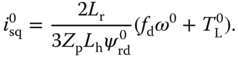
and  are first determined according to the operating conditions of the induction motor. Next, from (6.23), by letting
  , the steady-state solution of
  is determined via the steady-state calculation,
  . Furthermore, by letting
  , the steady-state operating condition for
  is calculated using (6.24) together with the linear approximation (6.31),
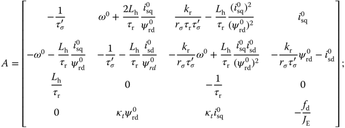
With all the steady-state operating parameters defined, the next step is to substitute (6.28)–(6.33) into (6.21)–(6.25) in order to obtain the linear time-invariant (LTI) model that is valid at the operating condition specified by the steady-state parameters  ,
,  ,
,  ,
,  . By gathering all the appropriate terms, it can be verified that the linear model has the form,
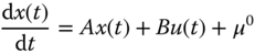
where  ,
, 
 , and with the coefficient
  , the matrices
  and
and  are defined as
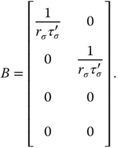
The constant vector  represents uncertainties associated with the physical parameters and the variations of the steady-state parameters. It is seen that the uncertainties are captured as input constant disturbances to the system.
6.2.5 Food for Thought
- Would you say that the first order Taylor series expansion underpins the linearization of nonlinear models?
- Would you want to a use second order Taylor series expansion to improve the accuracy of approximation?
- For the linear models derived from the double water tank system, what are the actual physical variables that are directly measured? What are the deviation variables we created?
- Is it a good strategy to choose the steady-state values of a nonlinear system according to the reference signals to the closed-loop control system?
- Would it be possible to find the steady-state values by solving the nonlinear dynamic equations, which can be achieved by building a Simulink program?
- For a complex system, would you consider using experimental tests to find the actual operating conditions through steady-state experiments?
6.3 Case Study: Ball and Plate Balancing System
This section is based on a final year project performed by Mr John Lee (see Lee (2013)), who was previously a fourth year electrical engineering student at RMIT University, Australia. As part of the project, a prototype of a ball and plate balancing system was built and PID control systems were designed for this self-made system. More importantly, they were successfully implemented with experimental results. Details for this project can be found in Lee (2013).
6.3.1 Dynamics of the Ball and Plate Balancing System
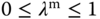
A ball and plate balancing system is illustrated in Figure 6.3, which consists of a ball and a rigid plate together with a set of actuators, sensors, and a controller. The position of the ball on the top of the plate is controlled by manipulating the inclination of the plate about its  - and
- and  -axes.
The system has four variables to be controlled. The first pair corresponds to the inclination of the plate in the  - and
- and  -axes captured by the angles of the plate
  and
and  from the
  - and
- and  -axes, and the second pair corresponds to the position of the ball in the
  - and
- and  -axes denoted by
  and
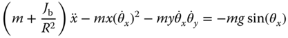
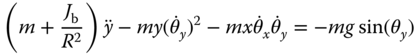
and  . Two DC motor drivers are used to control the system. The relationship between the motor torque forces and the inclination of the plate is described by the following two differential equations:


where  and
and  are the mass moment of inertia of the plate and the ball respectively,
  is the mass of the ball and
  is the gravity constant (
 m
m  ). The variables
  and
and  are the torque forces in the
  and
and  directions.
The movement of the ball on the plate is described the following two equations:
where  is the radius of the ball.

Figure 6.3 Schematic of the ball and plate balancing system.
In the control system implementation, a touch screen is used as the sensor to measure the ball's position on the plate. As a result, a heavy ball is used, which gives the inertial parameter  as
as
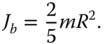
Thus, the plate dynamic equations are re-written as
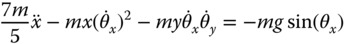

Clearly the equations 6.36 and (6.37) describe the actuator dynamics, which have severe nonlinearities, and the equations 6.40 and (6.41) describe the position outputs  and
and  in relation to the input variables
  and
and  . From these two sets of equations, it is apparent that cascade control systems (see Chapter 7) should be deployed to control the actuators and the plant, respectively.
However, because in the control system implementation two DC motors are used as the actuators with their angular positions under control from the manufacturer, the dynamics from the actuators are neglected and, instead, steady-state relationships between the angular positions of the DC motors and the inclination of the plate (governed by  and
and  ) are found. With this simplification, the control system design focuses on the dynamics of the plate as described by (6.40) and (6.41) where the inputs are
  and
and  , and the outputs are the positions of the ball governed by
  and
and  coordinates.
6.3.2 Linearization of the Nonlinear Model
The next step in the control system design is to derive the linear models for the nonlinear dynamic system. The operating conditions for the ball and plate balancing system are defined as follows.
- At the equilibrium, the ball is stable at the center of the plate, which is
 and
and  .
. - The angle of the plate is zero in both
 - and
- and  -axes, which is translated to
 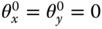 .
. - The angle of the plate is not changing, which leads to
 .
.
To obtain the linear model for (6.40), we consider the linearization procedure term by term.
The first term in (6.40) is linear by itself and does not require linearization. The nonlinear function in the second term is approximated by a Taylor series expansion as
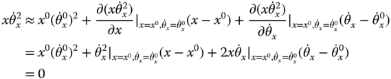
because 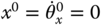 .
.
The quantity in the third term of (6.40) is approximated by a Taylor series expansion as
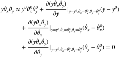
because  .
.
The nonlinear quantity on the right-hand side of (6.40) is approximated as
Combining all the linearized quantities together yields the linear model that describes the dynamics of the ball and plate balancing system at its operating condition as,
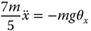
which says that at the equilibrium point, the ball and plate balancing system is a double integrator system. The input to the system is angle of the plate  and the output is the position of the ball
  on the plate.
The dynamic model for the  -axis is obtained through the linearization of the nonlinear model (6.41) as
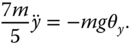
It is seen that the linearized models are equal. Also the coupling relationships in the original nonlinear models are gone, meaning that two identical PID controllers can be used to control the  - and
- and  -axes separately.
6.3.3 PID Controller Design
Because all the steady-state variables are zero in the ball and plate balancing system, the Laplace transfer function of (6.42) for the  -axis becomes

Because the system is a double integrator system, one might attempt to use a PD controller for the position control because the self-contained integrator would take care of the tracking accuracy to step reference signals. Were the system a true double integrator, this option would be viable. Because the double integrator is the result of linearization of a nonlinear model, a small deviation from the operating condition, this characteristic would disappear, observed from the original physical model (6.40). Therefore, PID controller with derivative filter is selected to perform the position control.
Following from the PID controller design in Section 3.4, the controller structure is selected as

and the desired closed-loop polynomial is selected as
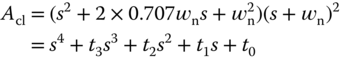
where the parameter  is a tuning parameter for the closed-loop performance.
With the second order model,

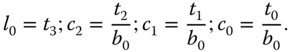
where  , the polynomial equation for solving the PID controller parameters becomes
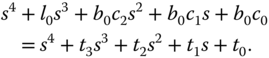
The solution of (6.46) gives
To determine the performance parameter  , using Simulink simulation, nonlinear system simulators were built with consideration of the nonlinear plant and actuator dynamics for various reference signals. It was found that
  is a satisfactory choice from the simulation studies based on the nonlinear simulators, and this
  was used in the actual implementation with a small adjustment for special cases.
It is noted that the linear models for the ball and plate balancing system are sufficiently accurate for the PID controller design with the parameter  calibrated against the nonlinear system. By adjusting
  , we effectively adjust the desired closed-loop bandwidth against the actual physical system to reduce the effect of modeling errors.
However, when a resonant controller is designed using the linear model (6.44), the feedback controller could not stabilize the actual physical system despite numerous attempts. A possible key reason for this problem is that the resonant controller demands much higher accuracy from the plant model in the higher frequency region. The neglected dynamics from the actuators and the sensors will have a greater effect on the closed-loop stability and performance when a resonant controller is used.
As a result, in order to track a sinusoidal reference signal, the same PID controllers are used with feedforward compensation on the reference signals, in which the output errors at the steady-state operation are measured and then compensated at the reference signal by modifying its amplitude and phase. This compensation from reference signal no longer puts extra demand on the accuracy of the model.
6.3.4 Implementation and Experimental Results
In the implementation of the control system, the parameters in controller (6.45) are converted to  ,
,  ,
,  and
and  for the discretization and a two degrees of freedom PID controller is implemented as shown in Section 3.4, which is to put the proportional control and the derivative control on the output only. The sampling interval used in the implementation is
  (s).
(s).
Additionally, to protect the equipment, constraints on the derivative of the control signal and the amplitude of the control signal are imposed with anti-windup mechanisms, which was shown in Tutorial 4.1. In the implementation, the MATLAB real time function PIDV.slx in Tutorial 4.1 was converted into C-code for real time execution using a micro-controller.
It was a tremendous effort to design and implement the ball and plate balancing control system, which requires detailed considerations and executions in hardware electronics design and software design. The design and implementation were detailed in Lee's report (Lee (2013)). As a case study, selected experimental results are presented.
6.3.4.1 Disturbance Rejection
In the disturbance rejection experiment, the ball is positioned at the center of the plate, which is at the coordinates of  and
and  . The reference signals to both
  - and
- and  -axes are zero and an external pulse disturbance was applied to the ball by using a finger to perturb the position of the ball. The
  -axis and
  -axis responses to this unknown disturbance are shown in Figures 6.4(a) and (b). Figure 6.4(c) shows the
  –
– plane plot for the disturbance rejection. It is seen that the PID control system has successfully rejected the disturbance without steady-state errors.
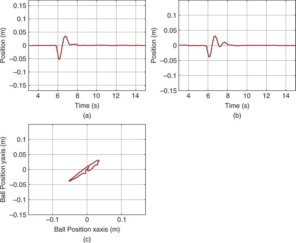
Figure 6.4 Disturbance rejection. (a)  -axis response. (b)
  -axis response. (c) Ball position.
6.3.4.2 Making a Square Movement
To make a square movement, two sets of step signals are chosen as the desired reference signals for the  -axis and
  -axis, as shown by the dashed lines in Figures 6.5(a) and (b). The output responses to the
  and
and  reference signals are compared in the same plots. Figure 6.5(c) shows the ball movement on the plate, which is seen as a square trajectory.
6.3.4.3 Making a Circle Movement
To make a circle movement, the reference signals to the  -axis and
  -axis are chosen to be
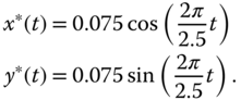
Here, the desired angular velocity of the ball movement is  rad s
rad s and the radius of the circle is 0.075 m.

Figure 6.5 Making a square movement. (a)  -axis response. (b)
  -axis response. (c) Ball position. Key: line (1) output response; line (2) reference signal.
As stated before, the closed-loop control using a resonant controller embedding the mode  into its denominator is not stable possibly due to modeling errors. The solution resorts to PID control with pre-compensation by modifying the reference signals.
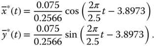
To find the suitable reference signals for the circle movement, the desired sinusoidal reference signals  and
and  are applied to the same PID control systems. Then, at steady-state operation, the ratio between the peaks of the reference and output is calculated as 0.2566, and the phase lag between the desired sinusoidal signal
  and
and  is 3.8973 rad. Therefore, the reference signals to the PID control systems are modified for the pre-compensation as
Figures 6.6(a) and (b) compare the  -axis and
  -axis responses to the original desired sinusoidal reference signals. Indeed, with the pre-compensation, the output signals track the desired reference signals quite nicely. Figure 6.6(c) shows the
  –
– plane movement of the ball, which is seen to make a circle movement.
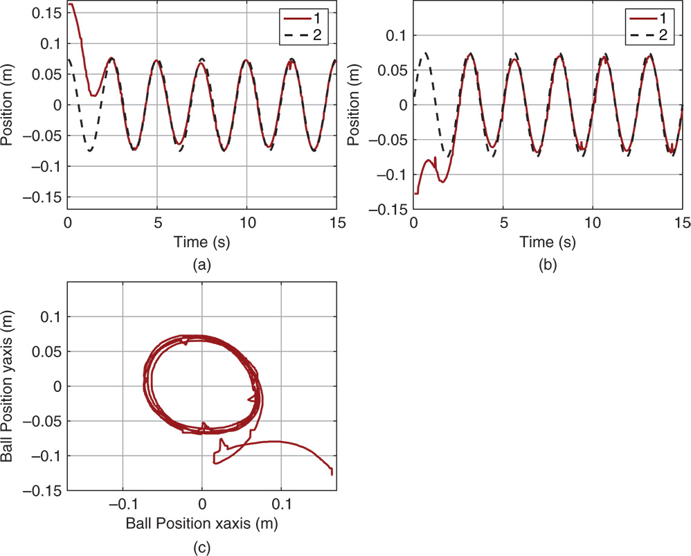
Figure 6.6 Making a circle movement. (a)  -axis response. (b)
  -axis response. (c) Ball position. Key: line (1) output response; line (2) desired reference signal.
6.3.4.4 Making more Complicated Movements
In the final year project thesis (Lee (2013)), the control of ball's square movement was extended to more complicated maze movement by carefully choosing the step reference signals on the  - and
- and  -axes. The control of ball's circle movement was extended to the movement of a figure “8”. They are all successfully implemented and validated on the ball and plate balancing system. For those who are interested in the other more complicated cases, Lee's video demonstration can be found at https://www.youtube.com/watch?v=wiPWqmlN5N4.
6.3.5 Food for Thought
- For the ball and plate balancing system, is it possible to choose other steady-state values for the linearization of the nonlinear model?
- Was it a bit surprise to find that the linear model for such a complex system is a simple double integrator with gain easily determined?
- Would you be able to list three factors that will result in modelling errors between the double integrator model and the actual ball and plate balancing system?
- In order to overcome the modelling error, which parameter do you think that John has used to tune the closed-loop PID controller against the actual ball and plate balancing system?
6.4 Gain Scheduled PID Control Systems
Gain scheduled control for nonlinear plants has proven to be a successful design methodology in many engineering applications. The gain scheduled control system is to use linear control strategies to control a nonlinear plant, and the family of closed-loop linear systems is stable in the vicinity of each linear model.
There are four general steps involved in the design of a gain scheduled control system listed as below, which are to
- identify the operating conditions of the nonlinear system and obtain a family of linear models with regard to these conditions;
- perform linear control system design for the family of linear models with specified closed-loop performance for each linear system;
- implement the actual gain scheduling that forms an interpolation between the family of the linear closed-loop control systems;
- validate and simulate the gain scheduled control system.
We have discussed the tasks given in step 1 and step 2 in the previous chapters. In this section, we will focus on step 3. Step 4 has been illustrated with experimental validations for induction motor control (see Wang et al. (2015)) and for a fixed-wing unmanned aerial vehicle (see Poksawat et al. (2017)).
6.4.1 The Weighting Parameters
One approach used in the design of a gain scheduled control system is to assign a set of weighting parameters with values between 0 and 1 that will correspond to each operating condition of the nonlinear system. These weighting parameters will be used in the next section for the calculation of the control signal with the gain scheduled component.
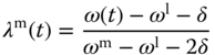
As an example, the gain scheduled speed control system for AC motor control is used for visualization. Here, the parameters  ,
,  , and
, and  are used as the weights for low speed, median speed, and high speed operations of a motor. The basic idea is to assign a correct value to the weighting parameters according to the operating conditions, which can be identified through the measurement of a physical variable. For the motor control application, its velocity is readily measured, which also influences the parameters of the linear model.
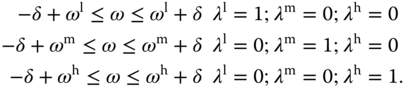
The first approach, also the simplest approach, is to assign the weighting parameters according to the reference signal of the system. We have following three cases. When we choose the reference signal  to be
to be  for low speed operation of the AC motor, then
  ,
,  and
and  . When we choose the reference signal
  to be
to be  for median speed operation,
  ,
,  and
and  . when the desired velocity is at the high speed where
  ,
,  ,
,  and
and  .
.
This approach takes into consideration the changes in plant dynamics due to reference changes; however, it does not consider the possibility that disturbances could cause the significant changes in plant dynamics. Hence, with this simple approach, closed-loop instability could occur if severe disturbances were encountered in plant operation.
The more general approach is to compute the weighting parameters  ,
,  , and
, and  according to the actual measurement of velocity
  . In order to avoid random triggering of the model changes in the presence of noises and transient responses, a band is formed around the desired speed. By assigning a tolerance constant
  to the desired speed ranges, the weighting constants
  ,
,  , and
, and  are defined as
Outside the band of the desired speed, none of the linear models can accurately describe the dynamic system. A traditional method is to use a combination of these two models from the nearest regions. For instance, assuming that the actual operating condition is between the band of the desired median speed and that of the desired high speed (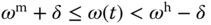 ), by defining
  (
( ) as a function of
  ,
,  is calculated using the linear interpretation of the two boundaries between the median and high speeds given by:
The weighting parameter  follows as
 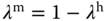 (
( ), and
  for this region. Similarly, for
 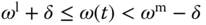 ,
,
and 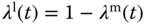 ,
, 
Figure 6.7 illustrates the weighting parameters that have been used to represent the operating regions of the AC motor.
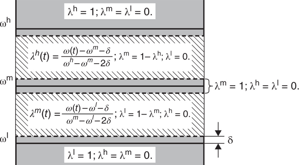
Figure 6.7 Weighting parameters.
6.4.2 Gain Scheduled Implementation using PID Velocity Form
One of the key elements in the implementation of a gain scheduled control system is that the calculated control signal is required to be the actual control signal, not the control signal in deviation variables. The difference between them is the steady-state value of the control signal  . Because when the operating condition changes the value
  changes, as we noticed from the exercises in linearization. This means that if we calculate the deviation control variable, this steady-state value needs to be adapted when the operating condition changes.
However, in the PID controller implementation shown in Chapter 4, the control signal was discretized with its steady-state value added to give the actual control signal, for example, see ((4.27)), which is shown at the sampling time  , as
, as

where the feedback error is calculated as  , and the derivative control signal
  is expressed in relation to the actual output signal
  as
as

Thus, the remaining task in the gain scheduled PID controller implementation is to perform the interpolation between the family of the linear closed-loop control systems.
We assume that with the three operating conditions selected, there are three PID controllers designed and simulated to obtain desired closed-loop performance for each operating condition. For clarity, we use the superscripts  ,
,  , and
, and  to denote the PID controller parameters obtained at the low, median, and high operating conditions. The identifiers
  ,
,  and
and  are calculated in real time using the actual output
  , which is equivalent to the velocity
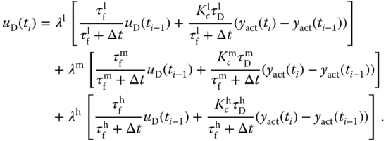
  in the previous section. Then, the calculation of the actual control signal with a gain scheduled controller becomes:

where  is calculated using the following scheduled expression:
To switch on the gain scheduled PID controller, the first sample of the control signal  will use the actual open-loop control signal, which is the estimate of the steady-state value
  at an operating condition. The values of
  ,
,  , and
, and  are continuously updated using the actual output or other physical parameter to pin-point the operating condition of the nonlinear system.
6.4.3 Gain Scheduled Implementation using an Estimator Based PID Controller
As an illustration, we will discuss the estimator based PI controller for the gain scheduled implementation. The extension to PID controller using an estimator is left as an exercise.
We assume that the system has three operating conditions denoted by the superscripts  ,
,  , and
, and  . At each operating condition, a first order model is obtained together with the steady-state values of the input signal
  and output signal
  .
.
At an operating condition, the steady-state values  and
and  are used to obtain the first order differential equation:

where  and
and  are the model coefficients obtained at the operating condition, and
  and
and  are the input and output deviation variables (or small signals), defined as

Note that in this formulation, the steady-state value  can be chosen to correspond to the reference signal at the operating condition, which is known in applications. It is more difficult to accurately determine the value of
  , but as in the velocity controller implementation, we can give a rough estimate of
  by using the initial open-loop control signal. Afterwards, the estimated constant disturbance
  in (6.52) will provide the compensation for the error in the steady-state value of the control signal
  .
.
As in Chapter 5, two desired closed-loop poles  and
and  are specified where
  . The controller and estimator parameters are calculated for the low speed operating condition as

for median speed operating condition as
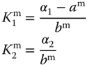
and for the high speed operating condition as

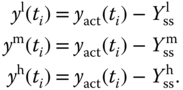
Because the control signal and output signal are small signals, they will be calculated in terms of their operating conditions. For this purpose, at the sampling instance  , we define the output signals for the three operating conditions:
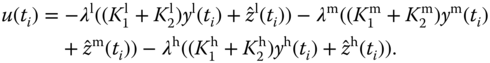
The control signal in deviation form is calculated using the identifiers  ,
,  , and
, and  introduced in Section 6.4.1 using the following form:
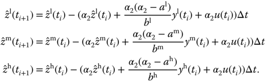
At sampling time  , the three estimators will run in parallel to estimate the disturbance term at different operating conditions:
The actual control signal is constructed using

The steady-state value  does not need to be accurate because of the estimation of disturbance. At the start of the closed-loop control, this parameter could take the value of the open-loop control signal. When operating condition changes, it can use the converged steady-state value of the control signal from the previous operating condition as the new steady-state value for the changed operating condition.
6.4.4 Food for Thought
- In the calculation of the weighting parameters,
 ,
,  and
and  , can we use other physical parameters beside the output variable, to identify the operating conditions?
 - In the gain scheduled PID controller when using the velocity form, do you need the steady-state information of the plant input and output?
- In the gain scheduled disturbance observer-based PID controller, do you need the steady-state information of the plant input and output?
6.5 Summary
Many physical models are represented by nonlinear differential equations. In order to design PID controllers for those physical systems, linearization of the nonlinear models is required. In this chapter, we have discussed how to obtain a linear model when a nonlinear model in the form of differential equations is given and how to design a gain scheduled control system for a nonlinear system. The other important aspects of this chapter are summarized as follows.
- An operating condition is selected to obtain a linear model for a given nonlinear model. A linear model is valid with respect to a chosen operating condition. If the operating condition changes, the linear model will change.
- In the linearization process, it is not always possible for us to find the correct equilibrium point due to parameter uncertainty. If this happens, we could model the uncertainty with a constant disturbance to the system. This constant disturbance will be overcome by the integral action in the controller or by subtracting it from the control signal with the disturbance estimation as proposed in Chapter 5.
- If the nonlinearity is severe, a gain scheduled control system is desired. With the gain scheduled PID control system, a family of linear models and controllers is obtained first, and the controller is smoothly switched when the operating condition changes. We can realize the gain scheduled PID control systems using the PID controller in velocity form or using the disturbance observer- based PID controllers.
6.6 Further Reading
- Text books for nonlinear control include Isidori (2013), Khalil (1996), Nijmeijer and Van der Schaft (1990).
- Henson and Seborg (1997) presents advanced topics in nonlinear process control.
- pH neutralization process is a typical example for nonlinear systems (Henson and Seborg (1994), Kalafatis et al. (1995), Böling et al. (2007)). It is a Wiener nonlinear model with its static inverse identified in Kalafatis et al. (1997), then compensated with the inverse nonlinearity, leading to a gain-scheduled control system (Kalafatis et al. (2005)). Another successful application of Hamerstein-Wiener model with a gain-scheduled control system is runtime management of Quality of Service (QoS) performance and resource provisioning in shared resource software environments (Patikirikorala et al. (2012)).
- The gain scheduled PID control algorithm presented in this chapter has been successfully used to attitude control of fixed-wing unmanned aerial vehicle with experimental validations (Poksawat et al. (2017)). The gain scheduled algorithm has an extension to continuous-time model predictive control, which was successfully validated on induction motor control (Wang et al. (2015)).
Problems
- 6.1 Perform linearization of the following differential equations and find their transfer functions at the operating conditions.
- A dynamic system is described by the following differential equation:

Find the linearized model at
 and
and  . Is this system stable at this operating condition?
 - A dynamic system is described by the following differential equation:

Find the linearized model at
 and
and  . Where are the poles of this linearized system?
- A dynamic system is described by the following differential equation:
- 6.2 Perform linearization of a differential equation for an inverted pendulum on a cart. The differential equations that describe the motion of an inverted pendulum are:
(6.54)
 (6.55)
where
 is the angle of the pendulum,
  is the horizontal position of the cart,
  is the length of the pendulum,
  and
and  are the masses of the cart and the pendulum, respectively, and
  is the moment of inertia of the pendulum about its center of gravity. F is a force applied to the body of the cart.
The operating point of the pendulum is selected as,
 , and
, and  , and
, and  .
.- Verify the linearized differential equations at the operating point are:
(6.56)
 (6.57)
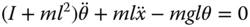
- Find the Laplace transfer function between the force
 (the input variable) and the pendulum angle
  .
.
- Verify the linearized differential equations at the operating point are:
- 6.3 A Permanent Magnetic Synchronous Motor (PMSM) is described by the differential equations in the d-q rotating reference frame:
(6.58)
 (6.59)
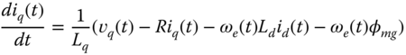 (6.60)
 (6.61)
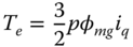
where
 is the angular electrical speed and is related to the rotor speed by
  with
with  denoting the number of pole pairs,
  and
and  represent the stator voltages in the d-q frame,
  and
and  represent the stator currents in this frame, and
  is load torque that is assumed to be zero if no load is attached to the motor.
The operating point for the PMSM is defined as
 ,
,  and
and  . Find the linearized differential equations that describe the dynamics of the motor at the operating point.
 - 6.4 A continuous-time system is described by the differential equation,
(6.62)

Supposing that the operating point for the input signal is at
 , the operating point for
  could be determined by letting
  and solving the algebraic equation with the value of
  , leading to(6.63)
- What is the operating point for
 ? Find the linearized model against the operating points of
  and
and  .
. - Find the Laplace transfer function between the input variable
 and the output variable
  . Is this system stable at the operating point?
 - Design a PI controller for this system, where the closed-loop poles are positioned at
 .
.
- What is the operating point for
- 6.5 A dynamic system is described by the following differential equation:

- Find the linearized model at
 and
and  . Hint: we need to consider the case
  and
and  separately to obtain two linear systems depending on the sign of the control signal
  .
. - Design two PID controllers for this system in terms of both positive
 and negative
  , where all closed-loop poles are positioned at
  (
( ), which is selected to produce stable closed-loop systems with satisfactory performance.
  could be different for the two controllers. A starting point is to select
  .
. - Implement the gain scheduled PID control system using the sign of control signal
 as the identifier of the operating condition. We modify the PIDV.slx real-time function to incorporate the gain scheduled control feature. In the simulation, the reference signal is chosen to be zero, and added to the simulation is an input disturbance, which is a square wave signal with appropriate period 2 and amplitude of
  . The sampling interval
  is selected to be 0.01.
- Find the linearized model at
- 6.6 Consider the linearized model and the nonlinear plant given in Problem 6.5.
- Design two disturbance observer-based PID controllers for the same nonlinear plant depending on the sign of the control signal, where all desired closed-loop poles for both controller and estimator are positioned at
 (
( ). The parameter
  , which could be different, is selected to produce stable closed-loop systems with satisfactory performance. A starting point is to select
  .
. - Modify the MATLAB real-time function PIDEstim.slx introduced in Tutorial 5.2 to include the gain-scheduled control feature. Simulate the closed-loop control system for input disturbance rejection with the same simulation condition outlined in Problem 6.5.
- Design two disturbance observer-based PID controllers for the same nonlinear plant depending on the sign of the control signal, where all desired closed-loop poles for both controller and estimator are positioned at