5
Disturbance Observer- Based PID and Resonant Controller

5.1 Introduction

In Chapter 1 to Chapter 4, we discussed PID control systems with explicit functions of proportional control, integral control, and derivative control. Because integral control embeds a marginally stable mode in the controller structure, which could cause the problem of integrator windup when the control signal reaches its saturation limits, the PID control system implementation requires modification to overcome this problem. Similar implementation problems to a worse degree are faced by the resonant controllers.

This chapter examines the PID controller design and resonant controller design from a different angle to the previous chapters. It introduces the integral mode and resonant modes through disturbance estimation. By doing so, the design becomes simpler, and more importantly, the implementations of the PID and resonant controllers flow naturally from the designs with anti-windup mechanisms. This development is particularly significant for resonant controllers because simplicity in the implementation with anti-windup mechanisms is paramount for practical applications.

5.2 Disturbance observer-Based PI Controller

This section introduces the idea of disturbance estimation that leads to an equivalent PI control system. The mathematical model used in this section is a first order model. For systems with higher order transfer functions, approximation is required.

5.2.1 Estimation of Disturbance with Control

We assume that there is a constant input disturbance images , which is unknown. So the differential equation used to describe a first order system is given by

(5.1)

where images and images are model coefficients, and images and images are the input and output variables. Figure 5.1 illustrates the mathematical model to be used for the estimator based PI controller design.

Because of the assumption that images is a constant, we have

(5.2)

Image described by caption and surrounding text. — **Figure 5.1** Block diagram of the system for a disturbance observer-based PI controller.

We would like to specify two desired closed-loop poles images and images where images . In the proposed design, the choice of images influences predominantly the proportional gain images and images predominantly the integral gain images .

5.2.1.1 Choice of Proportional Controller

The choice of images is straightforward. Firstly, we define:

(5.3)

Then (5.1) becomes

(5.4)

Together with proportional control

we obtain the closed-loop system:

(5.5)

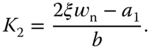
Equating the actual closed-loop pole images to the desired closed-loop pole images , we find the proportional gain images as

(5.6)

5.2.1.2 Compensation of Steady-state Error

We know that proportional control will lead to a closed-loop system with steady-state error for a constant reference signal or a disturbance signal. For overcoming the steady-state error, we need integral action incorporated into the control system. Here, we will estimate the steady-state error and then compensate it in the control signal. For this purpose, we extract the disturbance information from (5.1) leading to

(5.7)

One might attempt to directly calculate the unknown disturbance images using (5.7) and compensate for it in the control signal. However, it can be easily verified that such an approach fails to produce the control signal required because of uncertainties in the model parameters and other imperfections in practical applications. We will estimate the disturbance signal images with compensation on the error.

Let images denote the estimated disturbance signal. The error, between what is given and what is to be estimated, is described by,

(5.8)

With the gain images weighted on the error images , together with the assumption images , we construct the estimation images as

(5.9)

This is the so-called observer-equation. We will choose the gain images such that the error images converges to zero.

Note that

(5.10)

then, the parameter images is chosen such that images . This then leads to

Hence,

(5.11)

For any given initial condition images and images , the estimation error images as images . The convergence rate is dependent on the parameter images . The larger images is, the faster the error will converge to zero.

Now, to calculate the control signal with compensation on the steady-state error, the unknown disturbance images in (5.3) is replaced by the estimated images from (5.9), leading to the control signal calculated as

(5.12)

5.2.1.3 The closed-loop poles

To verify indeed that the closed-loop poles for the control system are images and images , substituting (5.12) into (5.1) gives

(5.13)

where images . Together with (5.11), the closed-loop system equation is written as

(5.14)

Because images is an upper triangular matrix, the closed-loop poles (or eigenvalues) are simply calculated as the solution of the characteristic equation:

where images is the identity matrix with dimensions images , equal to images and images .

5.2.1.4 Implementation procedure

Because the estimation equation 5.9 contains the derivative of the output signal images , direct discretization requires information of images at sampling time images , which is not available to us.

Let us define a variable images as

(5.15)

Then, substituting this variable into the estimation equation 5.9 yields

(5.16)

If the reference signal images , then both (5.15) and (5.16) are modified by replacing images with images . Furthermore, if the control signal images reaches its saturation limit, this saturation information is updated in the estimation of the disturbance images via (5.16). Figure 5.2 illustrates the block diagram of the control system using disturbance observer. For discretizaton, at sampling time images , the derivative images is approximated using the first order approximation as

Then, it follows that

(5.17)

The calculation procedure for control signal is summarized as follows. Choose initial condition for images at the beginning of the closed-loop operation. This could be selected to be zero if no other information is available. With the reference signal images and output signal images available at sampling time images , the control signal images is calculated recursively. The control signal is limited between images and images .

Calculate the estimated disturbance signal at sample as
Calculate the control signal using the following equation

Figure 5.2 Block diagram of the control system using a disturbance observer.
Implement the control signal saturation:
Update the estimation of disturbance for the next sampling instant as
Send the control signal for implementation. When the next sampling period arrives, the new measurement of the output is taken and the computation is repeated from step 1.

5.2.2 Equivalence to PI controller

In order to calculate the equivalent PI controller, the Laplace transform of images is expressed as

where images , and the Laplace transform images is

(5.18)

The Laplace transform of the control signal images becomes

which is

(5.19)

Thus, the equivalent PI controller is revealed as

(5.20)

The PI controller parameters are

where images and images . We can verify that the closed-loop poles are at images and images , which was the design specification.

Block diagram depicting Transfer function realization of the estimator based PI controller. — **Figure 5.3** Transfer function realization of the estimator based PI controller and is the saturation limiter.

Defining the coefficients images and images and the saturation limiter images , Figure 5.3 shows the transfer function realization of the PI controller with anti-windup mechanism, which calculates the control signal images based on the reference signal images and the output signal images .

5.2.3 MATLAB Tutorial for Implementation of a PI Controller via Estimation

The embedded PI controller via estimation will be used in the simulation studies with the Simulink environment.

Tutorial 5.1

This tutorial is to illustrate how to implement the estimator based PI control algorithm in real-time. The core of this activity is to produce a MATLAB embedded function that can be used in a Simulink simulation as well as in MATLAB real time implementation. The entire embedded MATLAB completes one cycle of computation for the control signal. For every sampling period, it will repeat the same computation procedure.

Step by Step

Create a new Simulink file called PIEstim.slx
In Simulink's directory of User-Defined Functions, find the icon of embedded MATLAB function and copy it to the PIEstim model.
Click on the icon of the embedded function, and define the input and output variables to the PIEstim model so that the embedded function has the following form:
```
function uCur = PIEstim(r,y,K1,K2,alpha2,a,deltat,umin,umax) 
```
where uCur is the calculated control signal at the sampling time , the first two elements (r and y) among the input variables are the measurements of the the reference and output signals at sampling time , K1 and K2 are the controller gain and estimator gain, deltat is the sampling interval, and umin and umax are the lower and upper limits imposed on the control signal uCur.
At the top of the embedded function, find Model Explorer among the Tools. When opening the Model Explorer, select Discrete for the Update method and input deltat into the Sample time; select Support variable-size arrays; select Saturate on integer overflow; select Fixed point. Click Apply to save the changes.
We need to edit the input and output data ports in order to let the embedded function know which input ports are the real time variables and which are the parameters. This editing task is performed using Model Explorer.
- click on r, on Scope, select Input, assign port 1 and size −1 complexity, Inherited type Inherit: Same as Simulink. Repeat the same editing procedure for the output signal y.
- The remaining five inputs to the embedded function are the parameters required in the computation. Click on K1, on Scope, select Parameter and click Tunable and click Apply to save the changes. Repeat the same editing procedure for the rest of the parameters.
- To edit the output port from the embedded function, click on uCur, on Scope, select Output, Port 1, Size −1, Sampling Model Sample based, Type Inherit: Same as Simulink, and click on Apply to save the changes.
In the following, the program will declare the variable that is stored in the embedded function during each iteration for their dimensions and initial values. zhat is the estimated disturbance at sampling time , which needs an initial value and is assigned to zero. Enter the following program into the file:
```
persistent zhat
if isempty(zhat)
  zhat=0;
end 
```
Update the estimation of . Enter the following program into the file:
```
 dhat=zhat+K2*(y-r); 
```
Update the control signal by combining the proportional control with the disturbance estimation. Enter the following program into the file:
```
uCur= -K1*(y-r)-dhat; 
```
Implement saturation with anti-windup mechanism. Enter the following program into the file:
```
if (uCur>umax)
 uCur=umax;
 end
if (uCur<umin)
 uCur=umin;
 end 
```

Calculate the for the next sample. Enter the following program into the file:

zhat=zhat-alpha2*zhat*deltat-(y-r)*(alpha2-a)*K2*deltat..
-alpha2*uCur*deltat;

5.2.4 Examples for Estimator based PI Controllers

Example 5.1

A continuous-time system is approximated by the following first order model:

(5.21)

where the time constant is 10 s. It is known that the system has a variable delay of which has a maximum value of 1 s and a neglected time constant with a maximum value of 5 s. Design an estimator based PI controller for this system and simulate the closed-loop control performance for unit step reference change and rejection of input disturbance having amplitude of 20.

Solution. Because this system has neglected time delay and time constant, this model uncertainty will limit the specification of desired closed-loop performance. A good starting point is to select the dominant closed-loop pole equal to the known pole of system, which is at . Hence, . The second desired closed-loop pole is determined using closed-loop simulations with the MATLAB real-time function presented in Section 5.2.3.

With , , and , the parameter is calculated as

The parameter is calculated as

With the parameter being selected as 0.1, 0.2, and 0.3, three values of are calculated as 10, 20, and 30.

By selecting the sampling interval (s) and using the Simulink simulator with the PIEstim.slx function built in Section 5.2.3, closed-loop simulation results are obtained for the worst case scenario where the plant transfer function used in the simulation is

In the simulation, the unit step reference signal enters the system at and the input disturbance enters the system at half of the simulation time. It is seen from the comparative results illustrated in Figure 5.4 that with the increase in , the closed-loop response speed for both reference following and disturbance rejection has increased. One can verify that further increase of will lead to the increased oscillations in the closed-loop response. is a good choice with respect to the model uncertainties.

Two graphs depicting Time (sec) on the horizontal axis, output and Control on the vertical axis, and curves plotted for 1 to 3. — **Figure 5.4** Comparison of closed-loop control performance using an estimator based PI controller with different values (Example 5.1). (a) Control signal. (b) Output. Key: line (1) ; line (2) ; line (3) .

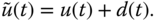
It is apparent that much larger control amplitude is required when images is used for the estimator based PI controller design. In practice, this much larger control amplitude may not be realizable due to the physical limitations of the actuators. An interesting question arises as how the closed-loop response speed will change if the control signal amplitude is limited. The following example illustrates the comparative studies.

Example 5.2

Continue from Example 5.1. Assuming that the control signal amplitude is constrained so that

(5.22)

Compare the closed-loop responses to a unit step reference signal and a step input disturbance with amplitude of 20.

Solution. We examine the slowest response case with and the fastest response case where is used for both cases.

When , the maximum and minimum of the control signal are naturally satisfied except for a brief time in disturbance rejection (see Figure 5.5). Therefore, for the choice of the closed-loop response to reference and disturbance signals remains unchanged with respect to the control signal constraints. However, when , the control signal amplitude exceeds its maximum and minimum values in reference following and disturbance rejection. In fact, the maximum value needs to be reduced from 35.60 to 14 and the minimum value needs to be increased from to . The constraints imposed will lead to a drastic reduction on the amplitude of the control signal when is used in the controller design. Figure 5.5(a) shows the closed-loop control signals to the step reference signal and the disturbance signal. It is seen that indeed the control signals are within the limits. Figure 5.5(b) compares the closed-loop responses to the step reference signal and the disturbance signal. It is seen that the closed-loop responses to the step reference signal have a similar speed, however, the disturbance rejection with the larger is much faster.

Two graphs depicting Time (sec) on the horizontal axis, output and Control on the vertical axis, and curves plotted for 1 to 2. — **Figure 5.6** Comparison of closed-loop control performance between the PI controller in velocity form and the disturbance observer-based PI controller (Example 5.3). (a) Control signal. (b) Output. Key: line (1) the PI controller in velocity form; line (2) the disturbance observer-based PI controller.

The above two examples indicate that with the estimator based PI control system, the closed-loop performance limitation is limited by the model uncertainties due to unmodeled dynamics in the system. The performance limitation is reflected by the value of images . The control signal limits can be incorporated into the implementation of the control system with a naturally occurred anti-windup mechanism.

From Section 5.2.2 it is clear that there is an equivalent PI controller with parameters images and images to this estimation based PI controller. The implementation of a PI controller using the velocity form was discussed with anti-windup mechanisms in Section 4.6. Naturally we wonder if these two implementations would lead to different outcomes. The following example compares the outcomes of these two PI controller with anti-windup mechanisms.

5.2.5 Food for Thought

In the design of a disturbance observer-based PI controller, what effect will the desired closed-loop poles and have on the closed-loop performance?
If the system has a large modelling error, would you decrease and ?
If the steady-state values of the control signal and output signal are not zero at the initial time, how would you enter these steady-state values in the disturbance observer-based PI controller implementation?
Is it possible to estimate the disturbance without compensating it in the control system?
Is the implementation of integrator based on a stable system?

5.3 Disturbance observer-Based PID Controller

To design a PID controller using the estimation based approach, we consider a second order transfer function:

(5.23)

where images and images are the Laplace transforms of the input and output signals. We assume that images . By assuming zero initial conditions, the corresponding differential equation is expressed as

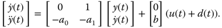
In matrix form, it is expressed as

(5.24)

5.3.1 Proportional Plus Derivative Control

We will first design a proportional plus derivative controller. For this purpose, the feedback control signal images is

(5.25)

Substituting (5.25) into (5.24) leads to the closed-loop equation:

(5.26)

The closed-loop characteristic polynomial is then calculated as

This is clearly a second order polynomial. We can specify a damping coefficient images and choose the parameter images as the closed-loop performance parameter. Alternatively, we could also choose two desired closed-loop poles as images and images where images and images . In any case, to determine the proportional and the derivative controller gain, the actual closed-loop characteristic polynomial is made equal to the desired one, leading to

The solution of this polynomial equation gives the proportional control gain:

(5.27)

and the derivative control gain:

(5.28)

Since it is necessary to use a filter for the derivative action because of measurement noise, a quick way to calculate a first order filter time constant is to find the corresponding gain images , which is

based on (5.25). With this parameter, the derivative filter constant is

where images is often selected. The filtered derivative output signal is expressed as

For many applications, it is preferable to design the PD controller together with derivative filter images to avoid the extra errors introduced from the approximation. A PD controller with filter design is discussed in detail in Section 3.4.1 with the filter constant calculated through the desired closed-loop performance specification.

5.3.2 Adding Integral Action

To add integral action to the PD controller, we assume that there is a constant input disturbance images so we have images . The differential equation model (5.24) is modified to become:

(5.29)

Similar to the PI controller design via estimation, we will write the unknown disturbance term as

(5.30)

Together with the assumption that images , the estimation of images is constructed as

(5.31)

We choose images and determine the estimator's gain images using

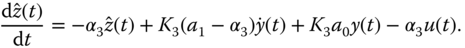
Because Equation 5.31 has double derivative and derivative of output signal images , it is not suitable for computational purposes. To this end, we define a new variable

and rewrite Equation 5.31 as function of images :

(5.32)

Assuming that the reference signal is images at the sampling time images and the output signal and its derivative are measured as images , images , with the sampling interval images , with saturation limits images and images , the control signal is calculated using the following steps.

Update the estimated disturbance signal. An initial condition on will be given as the start up of the control algorithm.
Calculate the control signal
Implement control signal saturation:
Update the disturbance estimator for :
When the next sample period arrives, repeat the computation at step 1.

Note that in the implementation of the PID controller, the derivative control is on the output only, avoiding producing a spike on the control signal when the reference signal signal images makes a step change. When a filter is used for the derivative signal images , the signal images is replaced by images , which is illustrated in Tutorial 5.2.

5.3.3 Equivalence to a PID Controller

To find the equivalence of the proposed estimation based PID controller to the PID controller expressed in transfer function form, we examine the Laplace transform of the estimation equation 5.31, which is,

(5.33)

where images . Solving for images gives

(5.34)

Note that the Laplace transform of the control signal is expressed as

(5.35)

By substituting (5.34) into (5.35), the Laplace transform of the control signal images is found as

(5.36)

With the negative feedback, the equivalent controller transfer function images is obtained as

(5.37)

Now, it can be verified that the closed-loop polynomial is indeed

(5.38)

where images and images are the numerator and denominator of the transfer function model as given by (5.23). Additionally, it can be verified that the controller transfer function can be written in an equivalent form to a PID controller:

(5.39)

where the parameters images , images , and images are calculated as

(5.40)

(5.41)

(5.42)

Figure 5.7 shows the transfer function realization of the disturbance observer-based PID controller where images is the saturation limiter.

There are several comments related. Firstly, the relationship presented in (5.38) shows that there are three desired closed-loop poles for the PID controller designed. The pair of complex poles located at images with images or 1 is used to determine the parameters images and images , and the pole located at images is used to determine the parameter images . Secondly, the PID controller can be implemented using the estimation of the input disturbance, providing a stable implementation for the integrator. Thirdly, the controller transfer function shown in (5.39) can readily be used for frequency response analysis so that the gain margin, phase margin, and delay margin can be calculated for the controller designed.

Block diagram depicting Transfer function realization of the disturbance observer-based PID controller. — **Figure 5.7** Transfer function realization of the disturbance observer-based PID controller.

5.3.4 MATLAB Tutorial on the Implementation of a disturbance observer-based PID Controller

This section presents the MATLAB tutorial for the implementation of disturbance observer-based PID controller. This implementation will contain the anti-windup mechanism when the control signal reaches its maximum or minimum values. The embedded PID controller via estimation will be used in the simulation studies within the Simulink environment.

Tutorial 5.2

This tutorial is to illustrate how to implement the disturbance observer-based PID control algorithm in real-time. The core of this activity is to produce a MATLAB embedded function that can be used in a Simulink simulation as well as in MATLAB Real-time implementation. The entire embedded MATLAB completes one cycle of computation for the control signal. For every sampling period, it will repeat the same computation procedure.

Step by Step

Create a new Simulink file called PIDEstim.slx
In Simulink's directory of User-Defined Functions, find the icon of embedded MATLAB function and copy it to the PIDEstim model.
Click on the icon of the embedded function, and define the input and output variables to the PIDEstim model so that the embedded function has the following form:
```
function uCur = PIDEstim(r,y,K1,K2,K3,tauf,alpha3,..
a1,a0,deltat,umin,umax) 
```
where uCur is the calculated control signal at the sampling time , the first two elements (r and y) among the input variables are the measurements of the the reference and output signals at sampling time , K1, K2 and K3 are the PD controller gains and estimator gain, tauf is the time constant for the derivative filter, alpha3 is for the pole location of the estimator, deltat is the sampling interval, umin and umax are the lower and upper limits imposed on the control signal uCur.
At the top of the embedded function, find Model Explorer among the Tools. When opening the Model Explorer, select discrete for the update method and input deltat into the sample time; select Support variable-size arrays; select Saturate on integer overflow; select Fixed point. Click Apply to save the changes.
We need to edit the input and output data ports in order to let the embedded function know which input ports are the real-time variables and which are the parameters. This editing task is performed using Model Explorer.
- Click on r, on Scope, select input, assign port 1 and size −1, complexity Inherited, type Inherit: Same as Simulink. Repeat the same editing procedure for the output signal y.
- The rest of 10 inputs to the embedded function are the parameters required in the computation. Click on K1, on Scope, select Parameter and click Tunable and click Apply to save the changes. Repeat the same editing procedure for the rest of the parameters.
- To edit the output port from the embedded function, click on uCur, on Scope, select Output, Port 1, Size −1, Sampling Model Sample based, Type Inherit: Same as Simulink, and click on Apply to save the changes.
In the following, the program will declare the variables that are stored in the embedded function during each iteration for their dimensions and initial values. zhat is the estimated disturbance at sampling time , which needs an initial value and is assigned to zero. We also declare the derivative of the filtered output and the past output signals that will be stored in the memory. Enter the following program into the file:
```
persistent zhat
if isempty(zhat)
  zhat=0;
end
persistent ydfpast
if isempty(ydfpast)
  ydfpast=0;
end
persistent ypast
if isempty(ypast)
  ypast=0;
end 
```
Update the filtered output derivative signal. Enter the following program into the file:
```
ydf=tauf/(tauf+deltat)*ydfpast+1/(tauf+deltat)*(y-ypast); 
```
Update the estimated disturbance . Enter the following program into the file:
```
dhat=zhat+K3*ydf; 
```
Update the control signal by combining the proportional plus derivative control with the disturbance estimation. Enter the following program into the file:
```
uCur= -K1*(y-r)-K2*ydf-dhat; 
```
Implement saturation with anti-windup mechanism. Enter the following program into the file:
```
if (uCur>umax) uCur=umax;end
if (uCur<umin) uCur=umin;end 
```

Calculate for the next sample. Enter the following program into the file:

zhat=zhat-deltat*alpha3*zhat+...
deltat*(K3*(a1-alpha3)*ydf+K3*a0*(y-r)-alpha3*uCur);

Update the past output signal and past filtered derivative output signal in preparation for the next sample period. Enter the following program into the file:
```
ypast=y;
ydfpast=ydf; 
```

This program is tested using the example presented in the next section.

5.3.5 Examples for Disturbance observer-based PID Controller

Example 5.4

An unstable system is described by the transfer function:

(5.43)

where the small time delay is due to the dynamics from the actuator. Design a estimator based PID controller with the pair of dominant poles at and the estimator pole at . Evaluate the control system performance for reference following and disturbance rejection in the presence of control amplitude constraints.

Solution. Choosing and positions the closed-loop poles at . The model (5.43) gives the parameters , , and . The PD controller parameters are calculated as

and the derivative control gain

Because it is an unstable system with neglected time delay, the selection of third pole is considered with simulation studies. When is too large, the neglected time delay will lead to the instability of the closed-loop system. However, when is not large enough, and the control amplitude constraints could lead to instability. The range of is found to be between 5 and 15 to provide satisfactory closed-loop performance in the presence of control signal amplitude constraints. With , the parameter is calculated as

A derivative filter time constant is calculated as

The filter time constant used is quite small because it introduces additional dynamics in the system. If the system has severe noises and a larger filter time constant is required, then the derivative filter needs to be designed as part of the control system (see Section 3.4.1). The disturbance observer-based PID control system is evaluated through simulation studies using the MATLAB real-time function in Section 5.3.4 together with a Simulink program. Choosing the sampling interval (s), in the simulation, a unit step reference signal enters the closed-loop system at and an input step disturbance with amplitude of 20 enters the system at half of the simulation time. The control signal amplitude is constrained between and 26. Figures 5.8(a) and (b) show the closed-loop control performances in the presence of the control signal amplitude constraints. In comparison, the responses from the unconstrained control signal and the output signal are also illustrated in the same figures. It is seen that the control amplitude has been reduced from about 100 to 26 at the beginning of the simulation. For the disturbance rejection, the control signal was constrained from the original to . The comparative results show that the constraints are met with little closed-loop performance deterioration.

One can also verify that the anti-windup PID controller implementation introduced in Section 4.6 will produce the same disturbance rejection results, however, will have a slower reference response if the proportional control is implemented on the output only. This is left as an exercise.

5.3.6 Food for Thought

In the design of disturbance observer-based PID controller, how would you modify Equations 5.29–(5.32) to include the derivative filter?
Can you list three physical systems that have second order transfer functions and are suitable for a PD controller application?
How would you propose to include the steady-state values of control signal and output signal in the implementation of the disturbance observer-based PID controller?
Would you consider the possibility of adding the integral action after the PD controller has stabilize the system, which can be achieved subsequently by subtracting the disturbance term?

5.4 Disturbance observer-Based Resonant Controller

This section will investigate resonant controller design and implementation with anti-windup mechanism using the disturbance estimation approach.

5.4.1 Resonant Controller Design

Assume that a dynamic system is described by the differential equation:

(5.44)

where images and images are the coefficients; images and images are the input and output signals; images is the input disturbance signal. In particular, we assume that images is a sinusoidal signal with known frequency images , but unknown amplitude images and phase angle images , which is expressed as

The resonant control law is expressed as

where images is an estimate of the unknown disturbance images .

By choosing the desired closed-loop pole at images and images , the proportional feedback control gain images is calculated as

Now, the next question is how to compute the estimated input sinusoidal disturbance signal images . The derivative of this disturbance signal is

and its second derivative is

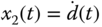Now, we choose images and images . With these choices, the following differential equations are used to describe the sinusoidal disturbance signal:

(5.45)

In order to estimate the disturbance signal images , from (5.44), we obtain

which is the output equation for the estimation. Thus, the estimated variables images and images are constructed as

(5.46)

where images and images are the estimator gains chosen for the design.

The next question is how to choose images and images such that the errors between the estimated and true disturbance signals are ensured to converge to zero as images . For this purpose, we define images and images . It can be verified as an exercise that we have the following error system:

(5.47)

where we have used the following relationship:

Clearly, we can choose the parameters images and images such that the poles (or eigenvalues) of the error system are on the left half of the complex plane, which ensures its stability. The characteristic polynomial for the error system is calculated as

Now, we choose a desired characteristic polynomial for performance specification as images . Then, to make the characteristic polynomial for the error system equal to the desired characteristic polynomial, the coefficients images and images are found as,

(5.48)

In the applications, the damping parameter images is chosen to be 0.707 and the parameter images is adjusted for how fast we would like to see the errors converge to zero.

5.4.2 Resonant Controller Implementation

The calculation of the estimated input disturbance using (5.46) requires the derivative of the output signal images , which is not desirable in the implementation. To overcome the problem, we define a pair of new variables:

Then, from (5.46), the following two equations are obtained:

(5.49)

(5.50)

The control law presented above is a combination of proportional feedback and a disturbance observer. This section will present how this control law can be implemented in a discrete time environment with anti-windup mechanism.

The derivatives in the observer equations 5.49 and (5.50) are first discretized with a sampling interval images leading to their approximations at the sampling time images :

The following algorithm summarizes the computational procedure for the implementation of the resonant controller with anti-windup mechanism.

Assume that the control signal images is limited to images and images , that is

Choosing the initial conditions for images and images , the control signal is calculated iteratively according to the following steps, where images is the reference signal at sampling time images .

Calculate the estimated sinusoidal disturbance as
Calculate the control signal as
Implement the saturations on the control signal using
Update the estimated disturbance signals using the following equations:
When the next sampling period arrives, repeat the computation from step 1.

5.4.3 Equivalence to a Resonant Controller

To find the Laplace transfer function of the resonant controller designed using disturbance estimation, we note that the Laplace transform of the control signal has the following expression:

(5.51)

where images is the Laplace transform of the estimated sinusoidal disturbance. It can be verified that the Laplace transform of (5.46) gives

(5.52)

Calculating the matrix inversion and multiplication gives

(5.53)

To find the Laplace transform of the control signal, we will substitute (5.53) into (5.51) and move the term containing images from the left-hand side to the right-hand side of the equation, which gives the expression of the control signal

(5.54)

where images and images .

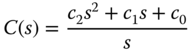
From (5.54), we find the Laplace transfer function of the resonant controller as

(5.55)

This controller has a pair of complex poles at images .

Block diagram depicting Transfer function realization of a resonant controller with saturation limits. — **Figure 5.9** Transfer function realization of a resonant controller with saturation limits.

To verify if the closed-loop poles are indeed at the locations of images and images ( images or 0.707), we calculate the closed-loop characteristic polynomial as

(5.56)

where images , images , and images . The closed-loop characteristic polynomial (5.56) leads to the conclusion that the closed-loop poles are at the locations as we specified.

Figure 5.9 shows the transfer function realization of the resonant controller with anti-windup mechanism.

5.4.4 MATLAB Tutorial on Disturbance observer-Based Resonant Controller Implementation

This section presents the MATLAB tutorial for implementation of the disturbance observer-based resonant controller together with the anti-windup mechanism when the control signal reaches its maximum or minimum values. The embedded resonant controller via estimation will be used in the simulation studies within the Simulink environment.

Tutorial 5.3

The core of this activity is to produce a MATLAB embedded function that can be used in a Simulink simulation as well as in MATLAB real time implementation. The entire embedded MATLAB completes one cycle of computation for the control signal. For every sampling period, it will repeat the same computation procedure.

Step by Step

Create a new Simulink file called ResEstim.slx
In Simulink's directory of User-Defined Functions, find the icon of embedded MATLAB function and copy it to the ResEstim model.
Click on the icon of the embedded function, and define the input and output variables to the ResEstim model so that the embedded function has the following form:
```
function uCur =ResEstim(r,y,K1,gamma1,gamma2,xi,wn,..
a,omega0,deltat,umin,umax) 
```
where uCur is the calculated control signal at the sampling time , the first two elements (r and y) among the input variables are the measurements of the the reference and output signals at sampling time , K1 is the proportional controller gain, gamma1, gamma2, xi, wn, a, omega0 are the parameters for the estimator, deltat is the sampling interval, umin and umax are the lower and upper limits imposed on the control signal uCur.
At the top of the embedded function, find Model Explorer among the Tools. When opening the Model Explorer, select discrete for the update method and input deltat into the sample time; select Support variable-size arrays; select Saturate on integer overflow; select Fixed point. Click Apply to save the changes.
We need to edit the input and output data ports in order to let the embedded function know which input ports are the real-time variables and which are the parameters. This editing task is performed using Model Explorer.
- Click on r, on Scope, select input, assign port 1 and size −1 complexity, Inherited type Inherit: Same as Simulink. Repeat the same editing procedure for the output signal y.
- The rest of 10 inputs to the embedded function are the parameters required in the computation. Click on K1, on Scope, select Parameter and click Tunable and click Apply to save the changes. Repeat the same editing procedure for the rest of the parameters.
- To edit the output port from the embedded function, click on uCur, on Scope, select Output, Port 1, Size −1, Sampling Model Sample based, type Inherit: Same as Simulink, and click on Apply to save the changes.
In the following, the program will declare the variables that are stored in the embedded function during each iteration for their dimensions and initial values. zhat1 and zhat2 are the two estimated variables at sampling time , which need initial values and are assigned to zero in this program. Enter the following program into the file:
```
persistent zhat1
if isempty(zhat1)
  zhat1=0;
end
persistent zhat2
if isempty(zhat2)
  zhat2=0;
end 
```
We calculate the following two constants using the parameters of the estimator. One could calculate the parameters outside the embedded function to save memory. Enter the following program into the file:
```
cz1=a*gamma1-2*xi*wn*gamma1+gamma2;
cz2=2*xi*wn; 
```
Update the estimated disturbance . Enter the following program into the file:
```
dhat=zhat1+gamma1*(y-r); 
```
Update the control signal by combining the proportional control with the disturbance estimation. Enter the following program into the file:
```
uCur= -K1*(y-r)-dhat; 
```
Implement saturation with anti-windup mechanism. Enter the following program into the file:
```
if (uCur>umax) uCur=umax;end
if (uCur<umin) uCur=umin;end 
```

Calculate the and for the next sample. Enter the following program into the file:

zhat1=zhat1+deltat*((-cz2*zhat1+zhat2)+cz1*(y-r)-cz2*uCur);
zhat2=zhat2+deltat*(-wn^∧2*zhat1..
+(a*gamma2-wn^∧2*gamma1)*(y-r)..
-(wn^∧2-omega0^∧2)*uCur);

This program is tested using the example presented in the next section.

5.4.5 Examples for Disturbance observer-Based Resonant Controllers

The following example is to illustrate the disturbance observer-based resonant controller design.

Example 5.5

An electrical system is approximated by the following first order plus time delay model:

(5.57)

where the delay is used to describe the neglected time constants from the other electronic components in the system. The control objective is for the output of the system to follow a sinusoidal reference signal with frequency . Design a resonant controller and simulate the closed-loop output with sampling interval (s).

Solution. The resonant controller is designed using the first order model, which gives the parameters and . Because the system has a time delay that is not used in the resonant controller design, it will affect the closed-loop stability and performance. Therefore, the proportional controller gain and the estimator gains need to be selected with regards to the actual first order plus delay system. A good starting point is to select the desired closed-loop pole for the controller gain equal to the model pole , leading to

Then, we select the parameters for the estimator to satisfy the closed-loop stability and performance in the presence of unmodeled time delay. By choosing , the parameter is used for adjusting the closed-loop response speed and robustness. The parameter selection can be performed using both closed-loop simulation and frequency response analysis.

One can verify that using the Simulink embedded function created in Tutorial 5.3, the closed-loop system is unstable for the choice of . Reducing to 500 gives the estimator gains as

Figures 5.10 (a) and (b) show the closed-loop control signal and the output signal to a sinusoidal reference signal with frequency . It is seen that the closed-loop system is stable. However the closed-loop responses are oscillatory in the initial period of responses evident from both the control signal and the output signal. The oscillation is caused by the neglected time delay in the plant.

Further reduction of is necessary to eliminate the undesirable characteristics. With the choice of , the estimator gains become,

Figures 5.11(a) and (b) show the closed-loop control signal and output signal to the sinusoidal reference signal. It is seen that the reduction of has eliminated the undesired behavior in both control signal and output signal.

Another approach to the selection of parameters and is to make , which could simplify the resonant controller tuning process. It can be verified through simulation studies that when , the closed-loop system has oscillatory modes. When the parameters are reduced to 400, the controller and estimator gains are calculated as

Figures 5.12(a) and (b) show the responses of the control signal and the output signal to the sinusoidal reference. It is seen that with this selection of performance parameters, the closed-loop system has satisfactory responses.

One can easily analyze the effect of unmodeled dynamics using the complementary sensitivity function together with the time delay (see Section 2.7). The nominal complementary sensitivity function is calculated using the transfer function . If for all , the following condition is satisfied:

where . Then, the closed-loop system is guaranteed to be stable. Figure 5.13 compares with respect to the two choices of the resonant controller parameters. It is seen that both closed-loop systems are robustly stable with for all .

Graph depicting Frequency (rad/s) on the horizontal axis, Mag on the vertical axis, and curves plotted for 1 to 2. — **Figure 5.13** (Example 5.5). Key: line (1) , ; line (2) .

It is clear that these two approaches in selecting the parameters images and images produced quite different controller parameters although the responses to the reference signal are similar. The question arises as how these two resonant controllers will behave in the presence of periodic disturbances. Clearly, if the disturbance has exactly the same frequency images , then both resonant controllers will achieve the same disturbance rejection at the steady-state operation from the sensitivity analysis in Section 2.5. However, when the actual disturbance frequency is different from images , there is a difference in the control system performance. The next example will compare the closed-loop performance of the two resonant controllers for the purpose of disturbance rejection.

Example 5.6

Continue from Example 5.5. Assuming that there is a sinusoidal input disturbance with its frequency in the range between and , we will evaluate the closed-loop performance of the two resonant controllers for the objective of disturbance rejection.

Solution. To measure how the resonant controllers will respond to disturbances in other frequency regions, we examine the sensitivity function

where is the frequency response of the system described by transfer function (5.57) and is the frequency response of the resonant controller described by the transfer function (5.55). Figure 5.14 compares the magnitude of the sensitivity functions for the two resonant control systems. Both sensitivity functions have a magnitude of 0 at from analytical solutions. For the choice of and , the sensitivity function has a lower gain at all frequency regions when comparing with the second case of . This implies that the first choice will work better for the purpose of disturbance rejections because smaller magnitude of sensitivity function leads to a better reduction of disturbance effect. Because the magnitude of the sensitivity function is not zero at the disturbance frequency band (, ), it is not possible to completely eliminate the disturbance with the resonant controller. To evaluate the actual closed-loop performance, an input disturbance

is added to the Simulink simulation program used in Example 5.5 where rad s. The rest of the simulation parameters and conditions remains unchanged from the previous example. Figures 5.15(a) and (b) compare the closed-loop output responses with the two resonant controllers. It is seen that the resonant controller designed using and produces much better reference tracking results than the one using . This improvement is the result of a better disturbance rejection property when the sensitivity function has a smaller magnitude at the disturbance frequency band.

In summary, for better disturbance rejection, one should select as large as possible, then adjust the bandwidth of the estimator to achieve closed-loop stability and performance in the presence of unmodeled time delay. We emphasize that the reason why the periodic disturbance is not completely rejected at the steady-state is because the actual disturbance frequency is .

The next example is to illustrate the effectiveness of the anti-windup mechanism contained in the resonant controller.

Example 5.7

Continue from Examples 5.5 and 5.6. The magnitude of the control signal is about 4.2 in order for the closed-loop system to track the sinusoidal reference signal and reject the sinusoidal disturbance. Assume that the physical system only allows the control signal to vary between , i.e.

Evaluate the resonant control system in the presence of control amplitude constraints.

Solution. The MATLAB embedded function presented in Tutorial 5.3 is used with the maximum and minimum values of the control signals specified. The rest of the simulation conditions remains unchanged from Example 5.6.

Figures 5.16(a) and (b) show the closed-loop resonant control system responses to the sinusoidal reference signal and the sinusoidal disturbance signal. It is seen that the control signal is constrained within the limits specified and the anti-windup mechanism works very well. Figure 5.16(b) reveals that despite the constraints imposed on the control amplitude, there is little performance loss in the output response to the reference signal.

5.4.6 Food for Thought

Can you list three systems that have first order dynamics and require a resonant control system for disturbance rejection or reference following of a sinusoidal signal?
Is it correct that with the disturbance observer-based resonant controller, the complementary sensitivity function has a magnitude of one at the frequency where is the frequency of the sinusoidal reference signal or the disturbance signal?
What do the closed-loop performance parameters and represent in the design of disturbance observer-based resonant controller? If there are neglected dynamics in the system, how would you choose them?
What are the key components in the disturbance observer-based-resonant controller that lead to the anti-windup mechanism in its implementation?
Would you say that it is quite straightforward to implement the resonant controller with anti-windup mechanism?

5.5 Multi-frequency Resonant Controller

In many applications, the resonant controller containing a single frequency introduced in Section 5.4 may not be adequate to track the reference signal or reject the disturbance signal that contains multiple frequencies. The framework we used in the single frequency case can be extended to multiple frequencies.

5.5.1 Adding Integral Action to the Resonant Controller

We consider the following first order differential equation as in Section 5.4

(5.58)

where images and images are the coefficients; images and images are the input and output signals; images is the input disturbance signal. Different from the resonant controller design, we assume that images is a combination of a sinusoidal signal with a constant. For this purpose, images is expressed as

where images and images is an unknown constant. The feedback control law is determined as

where images is an estimate of the unknown disturbance images .

With the desired closed-loop pole specified at images and images , the proportional feedback control gain images is given as

Now, we will extend the estimation algorithm presented in Section 5.4 to include the estimation of an unknown constant. Let us choose images and images and images . Note that images as images is a constant. The following differential equations will be used to describe the unknown disturbance images with the additional state images :

(5.59)

In order to estimate the disturbance signal images , from (5.58), we obtain

which is the output equation for the estimation. Thus, the estimated variables images , images , images are expressed as

(5.60)

where images , images and images are the estimator gains chosen for the design.

As in Section 5.4, we will choose the parameters images , images and images such that the poles of the error system are on the left half of the complex plane to ensure the convergence of the estimation errors. Here, the characteristic polynomial for the error system is computed as

(5.61)

where images , images for simplicity in the computation.

There is an analytical expression for the determinant given by (5.61), which leads to analytical solutions for the parameters images , images , and images . We firstly partition the images matrix into a block matrix as

where

With this partition, the determinant of the block matrix becomes

Note that images is exactly the same as the determinant described in the estimation of the sinusoidal signal in Section 5.4, which is

and the second determinant is

The characteristic polynomial for the closed-loop error system becomes

(5.62)

With the choice of desired characteristic polynomial for the performance specification that consists of a pair of complex poles and a real pole having the following form: images , we find the the coefficients images , images , and images as

(5.63)

The actual gains used in the estimation are then scaled to yield: images for images .

Defining images , images , and images , it can be verified that the implementation equation for the estimated disturbance becomes

(5.64)

where images is the system matrix defined as

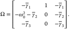
images has eigenvalues as the solutions of the characteristic equation:

Hence, the implementation of the estimator using (5.64) is a stable realization.

From the estimated images and images , we obtain

and images .

5.5.2 Adding More Periodic Components

If the system's disturbance or reference signal has more than one pair of periodic components, the disturbance estimator needs to be designed so to include those components.

We assume that the system is described by the differential equation 5.58. As before, images is the input disturbance signal and it is a combination of sinusoidal signals with a constant. For this purpose, images is expressed as

where images , images ( images ) and images is an unknown constant.

Continuing from the design in Section 5.5.1, we choose images , images , images , images , and images . With the two additional states, the following differential equation is used to describe the input disturbance images :

(5.65)

To estimate the disturbance signal images from the dynamic system (5.58), the disturbance term is written as

The estimated variables images , images , images , images , and images are written as

(5.66)

where images , images , images , images , and images are the estimator gains chosen for the design.

To find the estimator gains, we will consider the pair of matrices, images and images . Because of their higher dimensions, it is no longer easy to work out the analytical solutions of the estimator gains. Instead, we can use MATLAB programs for finding the estimator's gain matrix. For this purpose, we define the images and images matrices as illustrated in (5.66), and we choose five desired closed-loop poles for the error system to ensure the convergence of the estimated variables. The MATLAB program place.m is used to compute the images , images , illustrated as below:

Gamma=place(A',C',P)'

where images contains the five desired closed-loop poles for the error system and gamma is the vector that contains images , images .

5.5.3 Food for Thought

Is it correct that in the design of disturbance observer-based resonant controller for the multi-frequency signal, the complexity of the estimator has increased in order to estimate the multi-frequency disturbance signal?
Would you say that in general a higher accuracy of the model is required for estimating more frequency components?
Can you devise a resonant controller scheme for the multi-frequency control so that you can sequentially enter the periodic component one at a time?

5.6 Summary

We have discussed the PID and resonant controller design from the angle of disturbance estimation. Using the disturbance observer-based approaches, the integral control or the resonant control is introduced through the estimation of an input disturbance with the assumption that the disturbance is a constant for the integral mode or the disturbance is a sinusoidal signal for the resonant mode. The advantages of the proposed approaches include the simplified design for the controller, and perhaps even more importantly a stable controller structure suitable for direct implementation with an anti-windup mechanism in the event of control signal saturation. The other important aspects of the chapter are summarized as follows.

For a first order system with constant disturbance, the controller is a proportional control and the estimator is based on a first order model. This is equivalent to a PI controller with proportional and integral gains. The controller gain and estimator gains are selected with independent performance specifications.
For a second order system with constant disturbance, the controller has the functions of proportional and derivative control, and the estimator is based on a first order model. This is equivalent to a PID controller with proportional, integral and derivative gains. The closed-loop performance for the controller and the estimator is specified separately through the locations of their closed-loop poles.
For the resonant controller design, the system is assumed to have a first order model with input sinusoidal disturbance. The sinusoidal disturbance includes those with a single frequency or a multi-frequency. A proportional controller is used for the control function, and an estimator that embeds the sinusoidal modes is used to estimate the disturbance. This is equivalent to the resonant controller discussed in the previous chapters. Because the disturbance estimation is based on a stable system, the implementation of the proposed approach is numerically sound with a naturally embedded anti-windup mechanism if the control signal reaches its saturation limits.

For systems that have higher order dynamics, to use the design approaches proposed in this chapter, model order reduction is required.

5.7 Further Reading

A book is devoted to disturbance observer-based linear and nonlinear control systems (Li et al. (2014)). A survey is presented in Chen et al. (2016). The same research group has also worked on various topics of disturbance observer in control systems (Li et al. (2012), Yang et al. (2012)).
The early work on motion control using disturbance observer includes Komada et al. (1991). Disturbance observer is used for rigid mechanical systems in Schrijver and van Dijk (2002) and for robotic manipulator in Chen et al. (2000). Controller design for disturbance rejection is proposed using disturbance observer with estimation of frequency in Jia (2009). Stability and robust performance of motion control using disturbance observer is analyzed in Sariyildiz and Ohnishi (2015).
PID control and active disturbance rejection are introduced in Han (2009).
control is compared with disturbance observer-based control methods in Mita et al. (1998).
Disturbance rejection in dual-stage feed drive control system is discussed in She et al. (2011).
A recent survey is presented for disturbance estimation and attenuation in PMSM drives (Yang et al. (2017)) using the framework of disturbance observer.
The disturbance observer-based resonant controller is used to control a single phase voltage converter with experimental validation in McNabb et al. (2017).

Problems

5.1 Use the disturbance observer-based approach to design and implement a PI controller for the following systems:
1. Find the approximate first order model by neglecting the relatively small time constant(s) and small time delay while maintaining the same steady-state gain.
2. Choose the desired closed-loop pole for the proportional controller as where is the dominant pole for the system while the pole for the estimator is to obtain the estimator gain .
3. Compute the frequency responses of the controller , the sensitivity function , the input disturbance sensitivity function and the complementary sensitivity function . You can adjust the desired closed-loop poles for the controller and estimator, and observe their effects on the sensitivity functions.
4. Evaluate the closed-loop stability by using Nyquist diagram. If the closed-loop system is unstable, adjust the controller pole and the estimator pole to achieve stable closed-loop system.
5. Evaluate the robust stability condition for all :
6. What are your observations from the Nyquist diagram and robust stability condition? What can we do to improve the robustness of the closed-loop system?
7. Build the MATLAB real-time function PIEstim.slx by following Tutorial 5.1 and simulate the closed-loop step response and input disturbance rejection. We choose sampling interval and set the constraints on the control amplitude to be sufficiently large. A unit step reference signal is used in the simulation studies where a step input disturbance with amplitude of enters the simulation at half of the simulation time.
8. Evaluate the effect of constraints on the control signal where the constraint parameters and are chosen to be 85 percent of the control signal's maximum amplitude from the previous step.
9. What are your observations from the constrained control simulations?
5.2 Use the disturbance observer-based approach to design a PID controller for the following systems:
1. Choose the desired closed-loop characteristic polynomial for the proportional plus derivative controller as where and , while the pole for the estimator is to obtain the estimator gain .
2. Build the MATLAB real-time function PIDEstim.slx by following Tutorial 5.2 and simulate the closed-loop step response and input disturbance rejection with the sampling interval where the constraints on the control amplitude are set to be sufficiently large. In the simulations, the derivative filter time constant . The reference signal is a unit step signal and the input disturbance signal has amplitude of that enters the simulation at half of the simulation time.
3. Evaluate the effect of constraints on the control signal where the constraint parameters and are chosen to be 85 percent of the control signal's maximum amplitude from the previous step.
4. What are your observations from the constrained control simulations?
5.3 Consider the disturbance observer-based PID controller design for the three systems introduced in Problem 5.2. All the other conditions remain the same except designing the Proportional and Derivative controller with filter (see Section 3.4.1), where the filter time constant is considered in the process. The additional pole for the PD controller is chosen to be .
1. What are your observations on the PD controller parameters in comparison with those obtained from Problem 5.2?
2. Repeat the simulation studies with constraints as described in Problem 5.2 and compare the simulation results with those obtained from Problem 5.2. What are your observations?
5.4 It is ideal to incorporate the derivative filter in the PID controller design and analysis. From Section 5.3, inclusion of the derivative filter will change the transfer function of the PID controller presented in (5.39). Find the PID controller transfer function

that is equivalent to the disturbance observer-based PID controller.
5.5 Equation 5.18 reveals that the disturbance observer-based PI control is equivalent to computing the disturbance transfer function using the input and output signal:
(5.67)

which is, in essence, the inversion of the plant model together with a first order stable filter with unity steady-state gain for implementation, which is the essential component for disturbance observer-based approach (Li et al. (2014)).
1. Propose a discretization scheme for the disturbance estimation based on (5.67).
2. Draw a closed-loop feedback diagram with limits on the control signal amplitude. Does this implementation incorporate the anti-windup mechanism?
5.6 Equation 5.34 shows that the disturbance observer-based PID controller is equivalent to accessing the disturbance information with the following transfer function form:
(5.68)

which is the inversion of the plant model with first order filter that has a unity steady-state gain.
1. Propose a discretization scheme for computing the estimated disturbance based on the transfer function (5.68) with an additional first order filter so to make it realizable.
2. Draw the closed-loop diagram with control signal constraints.
5.7 From Problem 5.6, if the plant model has the following transfer function

where , and have the same sign, meaning a stable zero.
1. Express the in terms of the inversion of the new plant model.
2. Will this stable zero result in slow disturbance rejection if or if ?
3. Verify your answer by examining the input disturbance sensitivity function for both cases.
5.8 Consider the following systems with the given frequency for a resonant controller design:
1. Design the resonant controller based on a first order model by neglecting either the small time delay or small time constant (s), where the proportional controller pole is selected as and the desired closed-loop characteristic polynomial for the estimator as with .
2. Calculate the frequency response of the complementary sensitivity function and the multiplicative modelling error and check if the robust stability condition, for all :
  
  is satisfied. If not, reduce the parameter until it is satisfied.
3. Build the MATLAB real-time function ResEstim.slx by following Tutorial 5.3 and simulate the closed-loop response to a sinusoidal reference signal , where .
4. Add a sinusoidal input disturbance at half of the simulation time and simulate the disturbance rejection of the closed-loop system.
5. In order to evaluate the anti-windup mechanism, you may choose the control signal limits and based on 85 percent of the maximum and minimum of the control signal in transient response.
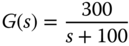
5.9 In many applications, tracking of a ramp reference signal is required. The disturbance observer-based resonant controller introduced in Section 5.4 can be modified to track a ramp reference signal by assuming the frequency . Assume that a given first order system is described by the following transfer function model:
1. Modify the disturbance observer-based resonant controller to track a ramp input signal;
2. Find the proportional controller gain by positioning the desired closed-loop pole at , and find the estimator gains and by choosing the desired closed-loop characteristic polynomial as , where and .
3. Use final value theorem to show that indeed this disturbance observer-based control system will track a ramp reference signal without steady-state error.
4. With the reference signal as , simulate the closed-loop response using the MATLAB real-time function ResEstim.slx where the sampling interval .
5.10 Consider the following first order system:

Design a resonant controller that will follow a reference signal , and reject an input disturbance , where all desired closed-loop poles for both the controller and the estimator are positioned at .
5.11 One application for the resonant controller is in the area of a single phase AC current regulator. The objective is to accurately track a sinusoidal reference signal with a frequency that matches the power grid.
The dynamic model for a single phase Voltage Source Inverter (VSI) coupled to a back electromotive force with an inductive-resistive filter network is expressed as

(5.69)

where is the output current from the inverter, is the input variable that is the pulse width modulated (PWM) switched voltage from the VSI, and is the back EMF voltage that is naturally a sinusoid with a nominal frequency . The parameter is the resistance and is the inductance, associated with the inductive-resistive filter network.

The control signal equals to the multiplication of a modulation signal with the inverter DC link voltage :

(5.70)

In the mathematical model of a single phase Voltage Source Inverter as in McNabb et al. (2017), the physical parameters are , , . The back EMF voltage is described by and ().
1. Design a resonant controller for the single phase Voltage source inverter, where . The closed-loop performance specifications are considered for the following two cases.
  1. The feedback controller gain is selected such that the closed-loop control system pole is equal to the open-loop system pole. The parameters for the estimator are and .
  2. The feedback controller gain is selected such that the closed-loop control system pole is twice of the open-loop system pole in magnitude. The parameters for the estimator are and .
2. Compare the sensitivity function and the complementary sensitivity function for the two cases. Determine the maximum time delay that the resonant control systems can tolerate. What are our observations? (Hint: the multiplicative modelling error is for neglected time delay ).
3. Choosing sampling interval (sec), simulate the closed-loop response to reference following and disturbance rejection, in which the reference signal is and the disturbance is . In the simulation model, the control signal is for simplification.
4. Impose the constraints on the amplitude of , where the maximum and minimum of the control signal are chosen to be 85 percent of the unconstrained control cases in transient responses.
5. Discuss the closed-loop control performances with respect to the two desired closed-loop performance specifications.