Chapter 4. Defying Reason
Photoshop Conversion Techniques of Mass Image Destruction: The Black and White on Convert to Grayscale, Split Channel Conversion, Lab Conversions, and Lab Equalization
There are no rules for good photographs, there are only good photographs.
—Ansel Adams
The Black and White on Convert to Grayscale
Pablo Picasso said, “Every act of creation is first an act of destruction.” But there is an exception to that belief, and it is epitomized in the next series of popular and very widely used conversion approaches. They contradict Picasso because even though you are engaging in an act of creativity, the following approaches are as creatively limiting as they are destructive to the image.
You should explore these approaches, rather than simply write them off as “too awful to use,” because they show some of the underpinnings of Photoshop and how tonal reproduction curves affect the image editing process. (See the sidebar: Terms of Engagement in Chapter 1 for a discussion of tonal reproduction curves.) The more information, the more experience, and better understanding that you have about how the whole process works, the greater the echo of that knowledge will be heard throughout your image editing process.
In Photoshop: Convert to Grayscale
The first of the destructive image conversion techniques is the Convert to Grayscale approach in Photoshop. When it comes to the color and luminance of your image files, Photoshop works by keeping all the color and luminance information as Lab (See the sidebar: From the Horse’s Mouth: Color Scientist Parker Plaisted Explains Lab vs. RGB later in this chapter) and then translates the file to the space that you have chosen (ProPhoto RGB, Adobe RGB, sRGB, Lab, CMYK, etc.).
When you convert a file to grayscale, using the Photoshop default setting, Photoshop converts the file (depending on the color space that the file is in) into one in which Red, Green, and Blue are weighted 30%, 60%, and 10% respectively. That means that Photoshop uses 30% of the Red channel’s information, 60% of the Green channel’s information, and 10% of the Blue channel’s information to create a grayscale image. This weighting is the equivalent of Photoshop’s tonal reproduction curve.
1. Open the image DSC0902_16BIT.tif (located in the Chapter 4 section of the download page for this book) (Figure 4.1).
Figure 4.1. Full color image
2. Click Save As (Command + Shift + S / Control + Shift + S), create a New Folder and name it DESTRUCTIVE_CONVERSIONS. Save the filename as GS_DSC0902_16Bit.psb and using the Large Document Format (.psb).
3. Go to Image > Mode and select Grayscale.
4. When the Discard Color information dialog box comes up, click Discard (Figure 4.2).
Figure 4.2. Grayscale image
You have just created a monochromatic image in which you have lost two-thirds of your image information. You should note that when you convert this file back to RGB in the next step, the file size will be the same as it was before you did the convert to grayscale.
5. Go to Image > Mode and select RGB.
6. Save the file (Figure 4.3 and 4.4).
Figure 4.3. File size of the full color image
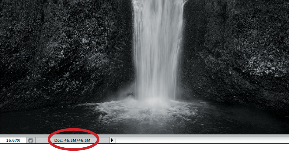
Figure 4.4. File size of the grayscale image
The reason that you convert back to RGB is so that you can make a print using all of the inks, not just the blacks.
The real goal of converting a full-spectrum color image into a chromatic grayscale one (one that never leaves the RGB color space) is to get as much information out of the file as your artistic voice requires.
The Black and White on Split Channel Conversions
It doesn’t matter how beautiful your theory is, it doesn’t matter how smart you are. If it doesn’t agree with experiment, it’s wrong.
—Richard P. Feynman
Earlier in the book, you saw that there is a difference between the Red, Green, and Blue channels as they are expressed in grayscale, and that when all three are combined, they create a full-spectrum color image. In this next destructive conversion technique, you are going to “split” out the image’s three color channels into three separate files, and then combine them into one master file.
1. Duplicate the file DSC0902_16BIT.tif (Image > Duplicate) and name it SPLTC_DSC0902_16BIT.tif.
2. Make the Channels panel active, click on the Channels Menu (located in the upper right corner of the Channels panel), and select Split Channels (Figure 4.5).
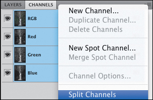
Figure 4.5. The Split Channels command
Photoshop will create three grayscale TIFFs, one for each of the Red, Green, and Blue channels. You will see that each channel is one-third of the file size of the original (Figures 4.6, 4.7, 4.8, and 4.9).

Figure 4.6. The original color image
Figure 4.7. The Red channel
Figure 4.8. The Green channel
Figure 4.9. The Blue channel
3. Make the SPLTC_DSC0902_16BIT.tif. Green file active. In the Layers panel, holding the Shift key down, click on the background layer and Shift-drag it to the SPLTC_ALL_DSC0902_16BIT.psd. Rename this layer GREEN and add a layer mask. Make the SPLTC_DSC0902_16BIT.tif. Green file active and close the file. When Photoshop asks you if you want to save this file, click No.
4. Make the SPLTC_DSC0902_16BIT.tif. Blue file active. In the Layers panel, holding the Shift key down, click on the background layer and Shift-drag it to the SPLTC_ALL_DSC0902_16BIT.psd. Rename this layer BLUE and add a layer mask. Make the SPLTC_DSC0902_16BIT.tif. Blue file active and close the file.
5. Make the SPLTC_DSC0902_16BIT.tif. Red file active and convert it back to RGB (Image > Mode > Grayscale to Image > Mode > RGB). Click on Save As (Command + Shift + S / Control + Shift + S) and rename the file SPLTC_ALL_DSC0902_16BIT. Save the file to the DESTRUCTIVE_CONVERSIONS folder and the file as a Photoshop Document (.psd).
This is a somewhat popular approach to chromatic grayscale conversion and, on the surface, it appears to make sense. It is completely reasonable to want to be able to access the grayscale representation of the Red, Green, and Blue channels so that they can be used to create a monochromatic grayscale image. Unfortunately, you wind up losing all of the underlying color information and therefore lose the ability to control how the colors of the image interact with each other once this conversion approach is done. While this technique seems reasonable, on the surface, doing this is akin to taking apart your watch without putting it back together again and expecting it to be able to tell time.
You can nondestructively, and with greater control, get the results used in the split-channel technique by creating three monochromatic Channel Mixers adjustment layers with the Red Channel set to 100% (Blue and Green set to 0), the Green Channel set to 100% (Red and Blue set to 0), and the Blue Channel set to 100% (Green and Red set to 0).
The only reason you would ever want to do this to an image (physically splitting the channels) would be for the purpose of using these split-out channels as a reference to help inform decisions using other types of chromatic grayscale conversions, specifically a Multi-Channel, Channel Mixer, adjustment layer approach that I will discuss later in this book.
A file that contains both the the split channels and the channel mixer adjustment layers set in monochrome mode for red, green and blue is named CH04_COMPARE.psb and is located in the Chapter 4 section of the download page for this book.
Even though your file is in RGB when you display the individual channels, they are displayed as grayscale documents, i.e., they are shown in the Grayscale workspace, not in the RGB workspace. So, even if you and I look at the same Adobe RGB document, each of us could see different channels if our grayscale setups were not identical. This is simply a programming error in the Channel Mixer algorithm.
Unless your grayscale gamma agrees with your RGB gamma, problems like grayscale workspace gamma versus RGB gamma are going to occur. Your only choice is to change your grayscale setting to agree with your RGB. In other words, if your normal RGB is Adobe RGB or sRGB, set your grayscale working space to 2.2 gamma. If it is ProPhoto, set it to 1.8. To do this go to Color Settings (Command + Shift + K / Control + Shift + K) and make the change.
The Black and White on Lab Color Space Conversions
If we observed first, and designed second, we wouldn’t need most of the things we build.
—Ben Hamilton-Baillie
Earlier in the book, you looked at how to create a black-and-white image by using the Hue/Saturation adjustment layer to desaturate the color. As you saw, simply desaturating the image’s color can be anything but simple. Even though you removed all of the color from the image, the workflow that you engaged in was non-destructive. Non-destructive image editing occurs when the original file content is not modified during the editing process—only the edits are edited. No matter what type of adjustment layer (e.g., Curves, Levels, etc.) you use, any time you do something to an image, you clip data. Your goal should be to develop a workflow that minimizes this and provides you with a direct path backward to the beginning.
Also, earlier in the book, you saw that there is a direct relationship between how you treat color and how that color manifests itself in the chromatic gray-scale. It is important, when conceptualizing a digital black-and-white image, to recognize that there is a difference between grays made up of varying shades or densities of black (printing with only black inks or just the lumance aspect of the image) and grays that are created out of equal values of red, green, and blue.
When you create a chromatic grayscale image from a full-spectrum color image, you are creating your own image-specific tonal reproduction curve. This is important because, as the creative force behind the image, you should decide how the colors in your image should interact, rather than use a predetermined, one-size-fits-all approach. You should know that when you make a part of an image a specific color, it will be rendered into a specific shade of chromatic gray in your final black-and-white print.
What you are working toward developing by doing every one of these conversion approaches is an ability to see a chromatic grayscale image while looking at one in color. This ability is frequently referred to as developing a visual framework. A visual framework is a global-to-granular approach that gets you from where you are to the vision that you have for your image, which in this case is an optimal chromatic grayscale print.
In this next approach, frequently referred to as the classic black-and-white conversion technique, and is one of the most widely used conversion approaches, you are going to create a chromatic gray-scale image in the Lab color space. This workflow is highly destructive, not because you will leave the RGB color space for the Lab color space, but because you will convert this image from Lab color, manually discard the a and b channels, then convert to grayscale in Photoshop using Photoshop’s convert to grayscale algorithm, and then back to RGB.
So exactly how much data would be lost from a color image if all the color is removed, and all that is left is the luminance information represented in grayscale? The answer again is that two-thirds of the data is lost. Photoshop works by keeping all the color/luminance information as Lab and then translates it, as necessary, into ProPhoto, RGB, CMYK, sRGB, Grayscale, etc. If you want to see this in action, convert an RGB image into Lab and then go to the Info panel. Apply the Desaturate command, which discards the a (green-magenta) and b (blue-yellow) color channels and retains only the L channel. Two of three channels are lost (thus two-thirds are lost) and the file size shrinks accordingly. Translating the file back to RGB yields a file of the original size. This is because the L channel has been represented in R, G, and B. All Photoshop had to work with, data-wise, was the L channel, so that you have equal values of R, G, and B in all three channels. The same thing happens if you convert RGB to gray-scale; the file size is reduced by two-thirds. Because converting an image straight to grayscale is so destructive, it should not be considered as a useful way to create a black-and-white image.
The Classic Black-and-White and Neo-Classic Black-and-White Conversion Approaches: Two Destructive Pathways to Getting the Hue Out of an Image
A jug fills drop by drop.
—Buddha
Using the equal color values test image that you used in the first chapter (RGB_TARGET.psd) I have created a file named RGB_TARGET_COMPARE.psb (located on the Chapter 4 section of the download page) so you can compare simple desaturation, the Red, Green and Blue channels with this next conversion approach. You should see that you have two different sets of gray values. If you look at the Red, Green, and Blue channels of the this Lab converted image, you will notice that each channel produces a different gray-scale image (Figures 4.10, 4.11, 4.12, and 4.13).
Figure 4.10. Original color image
Figure 4.11. Red channel
Figure 4.12. Green channel
Figure 4.13. Blue channel
When you do the classic black-and-white conversion technique in the Lab color space, only the luminance channel data should be extracted.
You can achieve this same result by creating a Hue/Saturation adjustment layer and setting the Saturation slider to -100.
Look at the color test file converted using individual channels in the Lab color space, the image converted using the Classic Black-and-White Conversion (Approach 1), and the image converted to grayscale (Figures 4.14, 4.15, 4.16, 4.17, 4.18, and 4.19).

Figure 4.14. L Channel

Figure 4.15. a channel
Figure 4.16. b channel
Figure 4.17. After the Classic Conversion process
Figure 4.18. Converted to Grayscale process
Figure 4.19. RGB file fully desaturated
You should see that the L (luminance) channel and the Classic Black-and-White Conversion 1 are identical, and that the Classic Black-and-White Conversion 1 and Convert to Grayscale from RGB are different. You should also notice that the Luminance channel in Lab renders different gray values for colors of the same value, whereas when the RGB version of this file was desaturated, all of the colors that were different became the same gray (Figures 4.10 and 4.19).

Figure 4.10. Original color image
It appears that Photoshop applies a tonal reproduction curve to the Luminance channel in the Lab color space. You will notice this because: first; all the colors in the test file are of equal luminance, but they appear to be different grays in the Luminance channel, and second; the 128 middle gray value that is the background of the test file is now lighter. What happened is that Photoshop applied a tonal reproduction curve to the L channel. Although the criteria used by Photoshop to determine this curve may not be important to you, you should know that the same tonal reproduction curve will be applied to every image that is converted this way. At first glance, it appears that the tonal reproduction curve is biased towards the a channel, because the red values of the test file tend to be a lighter gray. The problem here, just as it is with film, is that you cannot change the tonal reproduction curve.
Regardless, what you end up with is an image that has been arbitrarily changed to grayscale and one in which you have lost two-thirds of your image data. That is a lot of work for such little return.
If you look at the outcomes of the two variations of the Classic Black-and-White Conversion techniques in the Lab color space (that you are about to do), you will see that the results differ. The second approach will yield a darker image than was achieved with the first. However, when you compare the second approach to Photoshop’s Convert to Grayscale, the results are the same. So, once again, you will have done a lot of work to achieve something that can be more simply done elsewhere in the software. In addition, you still end up with a less than optimal result.
In the second way to do a Classic Black-and-White Conversion in the Lab color space, you should note that Photoshop has, again, applied a tonal reproduction curve. It appears that this curve tends to err in the direction of the b channel. And, once again, the result will be less than satisfying.
It important to know how to do both of these approaches because they are both extremely popular ways to do a black-and-white conversion and are touted by many professional photographers as the most accurate ways to create a realistic looking, black-and-white image. When you are finished with these techniques, you will find that you can get a quicker, better result by using two Hue/Saturation adjustment layers (as you did in Chapter 2) and changing the blend mode, than you can by using these conversion techniques.
Classic Black-and-White Conversion: Approach One
There are three classes of people: those who see, those who see when they are shown, those who do not see.
—Leonardo da Vinci
(For both Conversion One and Two you will use an image of the actor, Stephen Kearin.)
In the action set that comes with this book, there is an action that does this conversion. The action is named RGB_TO_LAB_TO_RGB and it is part of the OZ_2_K action set that is located in the ACTIONS folder that you should have downloaded from the download page for this book.
1. Open the file KEARIN.tif.
2. Duplicate the file (Image > Duplicate).
3. When the Duplicate dialog box comes up, name the file KEARIN_LAB_BW_1.
4. Click on Save As (Command + Shift + S / Control + Shift + S) and save this file in a Large Document format (.psb) to the DESTRUCTIVE_CONVERSIONS folder.
5. Go to Image > Mode and select Lab Color (Figure 4.20).
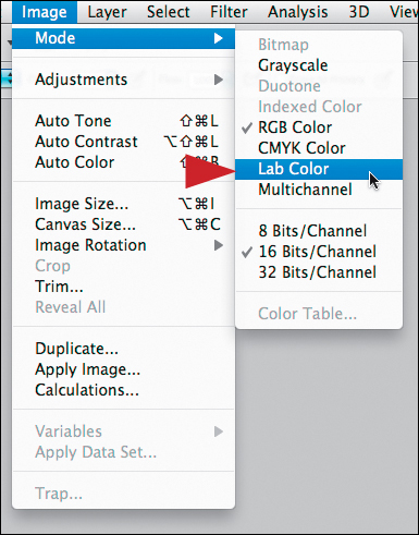
Figure 4.20. Converting to Lab Color
6. Select Channels and, holding down the Shift key, make the a and b channels active. Drag them to the Trash Can located at the bottom of the Channels Panel to discard them (Figure 4.21).
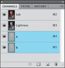
Figure 4.21. Selecting the a and b channels
See the difference before and after the a and b channels are discarded (Figure 4.22 and 4.23).
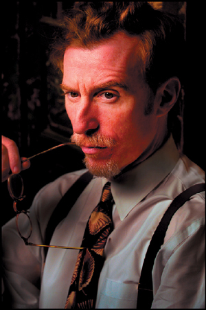
Figure 4.22. Before the a and b channels are discarded
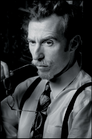
Figure 4.23. After the a and b channels are discarded
7. Go to Image > Mode > Grayscale (Figure 4.24).
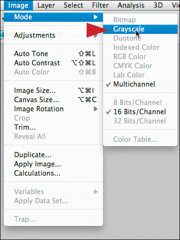
Figure 4.24. Convert to Grayscale
8. Go to Image > Mode > RGB Color (Figure 4.25).
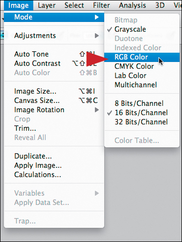
Figure 4.25. Convert to RGB
9. Save the file.
Now that you have converted this image, look at its individual RGB channels, its individual Lab channels, and the image converted to grayscale. Here is what the image’s individual RGB channels looked like before conversion and here is what they look like after the conversion process (Figures 4.26, 4.27, 4.28, 4.29, 4.30, 4.31, 4.32, 4.33, and 4.34).
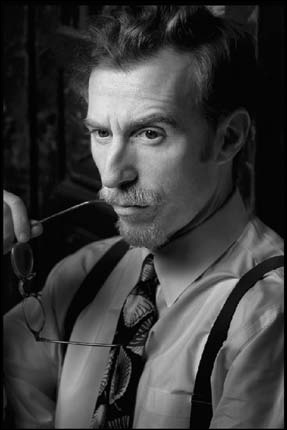
Figure 4.26. Red channel before conversion

Figure 4.27. Green channel before conversion

Figure 4.28. Blue channel before conversion

Figure 4.29. The Red channel after conversion

Figure 4.30. The Green channel after conversion

Figure 4.31. The Blue channel after conversion
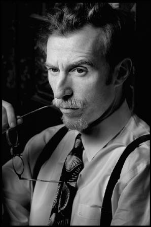
Figure 4.32. The L channel
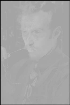
Figure 4.33. The a channel
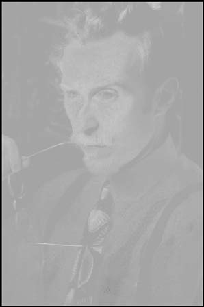
Figure 4.34. The b channel
Compare the final image to the Luminance Channel and you will see that they are the same (Figures 4.35 and 4.36).

Figure 4.35. Final image

Figure 4.36. Luminance channel
There is a file named LAB_COMPARE_100ppi. psb that is available on the download page; it has all the conversions as individual layers, which you can look at and compare.
Classic Black-and-White Conversion: Approach Two
Ignorance is no excuse, it’s the real thing.
—Irene Peter
In the action set that comes with this book, there is an action to do this. This action is named LAB_DISCARD_AB.
1. Open the file KEARIN.tif.
2. Duplicate the file (Image > Duplicate).
3. When the Duplicate Dialog box comes up, name the file KEARIN_LAB_BW_2.
4. Click on Save As (Command + Shift + S / Control + Shift + S) and save this file in a Large Document format (.psb), and in the DESTRUCTIVE_CONVERSIONS folder.
5. Go to Image > Mode > Grayscale.
6. When the Discard Color Information dialog box comes up, click OK.
7. Go to Image > Mode > RGB.
8. Save the file.
Now that you have converted this image, once again look at its individual RGB channels, its individual Lab channels, as well as the image converted to gray-scale (Figures 4.37, 4.38, 4.39, 4.40, 4.41, 4.42, 4.43, 4.44, and 4.45).

Figure 4.37. The Red channel before conversion

Figure 4.38. The Green channel before conversion
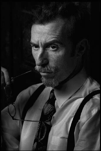
Figure 4.39. The Blue channel before conversion

Figure 4.40. The Red channel after conversion

Figure 4.41. The Green channel after conversion
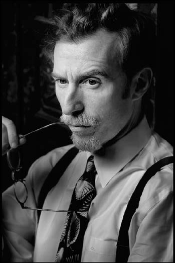
Figure 4.42. The Blue channel after conversion

Figure 4.43. The L channel
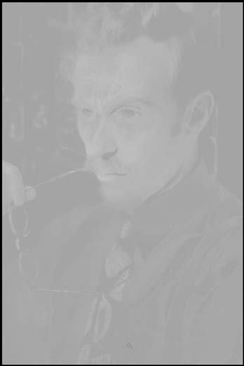
Figure 4.44. The a channel
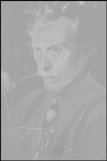
Figure 4.45. The b channel
Compare the final image to the converted to gray-scale image, which was created with Photoshop’s convert to grayscale technique, and you will see that they are the same (Figures 4.46 and 4.47).

Figure 4.46. The final image

Figure 4.47. The image converted to grayscale
You can see this comparison, as well, in the LAB_COMPARE_100ppi.psb file located in the Chapter 3 section of the download page.
The Black and White on Equalizing Lab
In a full color image, the use of the Lab color space is one of the most important tools for maximizing the image’s color information. There is no better way to increase an image’s color saturation than in the 16-bit Lab color space.
In the next part of this lesson, you will equalize all of the Lab channels. The Equalizing Lab technique can be quite useful when working on a chromatic grayscale-converted image derived from a color image, because it can create a layer that is lighter but one that has considerable detail. It can also create a lightened image that is far less contrasty than using the Screen blend mode to lighten. The Equalizing Lab approach to lightening an image is excellent for maintaining image structure and detail in the highlights, as well as in the shadows. Should you find that using either the Screen blend mode or Curves does not give you exactly what you want, consider using this approach.
The Equalize command works by redistributing the brightness values of the pixels in an image so that they more evenly represent the entire range of brightness levels. In other words, Equalize remaps pixel values in the composite image so that the brightest value represents white, the darkest value represents black, and intermediate values are evenly distributed throughout the grayscale.
In both the OZ2K and the OZ_POWER_TOOLS action sets for this book, there are actions to do both Lab Equalization and RGB Equalization. Even though I have found that Equalization is best suited for black-and-white images, from time to time it has been useful for full color images as well.
1. Duplicate the image file KEARIN.tif.
2. Rename this file KEARIN_Lab_EQ, and save it to the DESTRUCTIVE_CONVERSIONS folder.
3. Double-click on the Background layer and rename it Lab_EQ.
4. Desaturate the image (Shift + Command + U / Control + Shift + U).
5. Set the blend mode in the Layers panel to Luminosity.
6. Convert to Lab (Image > Mode > Lab color) (Figure 4.48).

Figure 4.48. The image in Lab mode
7. Go to Image > Adjustments > Equalize.
Compare the figures shown here (Figures 4.49, 4.50, 4.51, 4.52, 4.53, 4.54, 4.55, 4.56, 4.57, and 4.58).

Figure 4.49. Before equalization
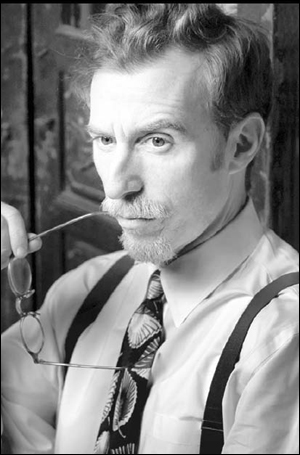
Figure 4.50. After equalization

Figure 4.51. RGB equalization
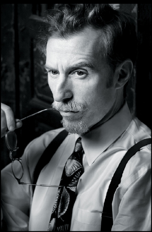
Figure 4.52. The Screen blend mode
Figure 4.53. Closeup of Lab equalization
Figure 4.54. Closeup of Lab equalization
Figure 4.55. Closeup of Lab equalization
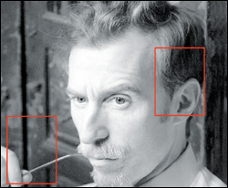
Figure 4.56. Closeup of RGB equalization
Figure 4.57. Closeup of RGB equalization
Figure 4.58. Closeup of RGB equalization
Here is where equalization becomes useful. I have created a version of the KEARIN.tif image using the third variation of the Film & Filter Approach (a layer with equal values of RGB, in this case white, set to the Color blend mode with a Hue/Saturation adjustment layer set to the Normal blend mode) that you learned in Chapter 2, that you will use for the next lesson. The file KEARIN_CB_BW_16BIT.psb is located in the Chapter 4 section of the download page for this book. I have also created a Curves adjustment layer that is turned on and is set to the Screen blend mode. (This halves the density of the image, and therefore causes the image to be lighter.) (Figures 4.59 and 4.60).

Figure 4.59. Before
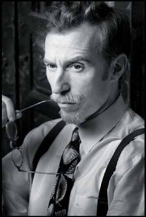
Figure 4.60. With Curves adjustment
When the Screen blend mode is applied however, even though the image is lightened, its shadow areas are still blocked up and the highlight areas become blown out. Be sure to look at the image when the Color blend mode layer is turned off in order to see what the actual colors look like (Figures 4.61, 4.62, and 4.63).
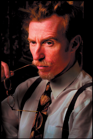
Figure 4.61. Original color image
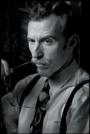
Figure 4.62. Color blend mode conversion with COLOR_BLEND_BW layer
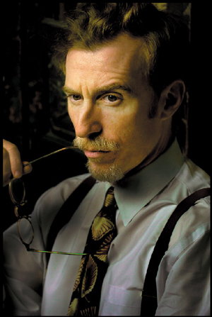
Figure 4.63. COLOR_BLEND_BW layer turned off
8. Open the KEARIN_CB_BW_16BIT.psb.
9. Turn off the SCREEN Curves adjustment layer.
10. Turn on the L2D_SCREEN adjustment layer (Figures 4.64 and 4.65).
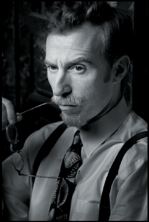
Figure 4.64. The image with the L2D_SCREEN layer on

Figure 4.65. The layer mask
11. Make the KEARIN_Lab_EQ file active, go to the Layers panel, and, holding down the Shift key, click on the Lab_EQ layer, and Shift-drag it to the KEARIN_CB_BW_16BIT.psb file.
12. Holding the Option / Alt key, drag the L2D_SCREEN layer mask to the Lab_EQ layer. Lower the opacity until you like the brightness. I chose 69%.
13. Save the file.
You duplicated the layer mask rather than painting a new one because you had already made choices about what looked best bright and what looked best dark, and so on. So rather than re-inventing the wheel, you saved time by duplicating the layer mask that you had already created. You can always do more brushwork on the layer mask you copied. This just gives you a place to start.
Of all the things that you can do to an image intended to be a chromatic grayscale image in the Lab color space, it is my opinion that equalizing in Lab is the most useful. It is also something that is best done when other less destructive ways of doing things, do not work as well as you had hoped.
There is a file named kearnin_all.psb that compares convert to grayscale, RGB desaturation, and both Lab conversion approaches. This file is located in the Chapter 4 section of the download page for this book.
The Bottom Line
Education is a weapon whose effects depend on who holds it in his hands and at whom it is aimed.
—Joseph Stalin
Converting an image from RGB to Lab to grayscale to RGB is a long, highly destructive, overly complicated task that involves losing two-thirds of your image data, as well as loosing the ability to control the relationship of color as it translates into a chromatic grayscale image. Of the three approaches that I have described, the first one is the only one that has some merit, if (for some reason) you are in need of the L channel data. The third one is useful if you need to pull image structures out of shadows and brighten highlight areas without losing image detail. But as chromatic grayscale conversions go, what these techniques are good for is showing how not to do something, and what happens when you make something simpler than possible.
When it comes to manipulating color, increasing saturation, or sharpening an image, there is no better color space in which to work than Lab. Enhancing color in Lab tends to look more natural and less noisy because the computation is carried out independent of luminosity. This cannot be done in RGB’s Luminosity mode, because it is designed to be perceptually uniform. When converting an image to chromatic grayscale, however, perceptual uniformity is exactly what you want, because you want to bend the colors of the image to your will and not be bound by the tonal reproduction curve applied by Photoshop.
