Exploring the Wilson-Cowan Equations
In this chapter, we will apply phase plane analysis to a model of two interacting neuronal populations, an excitatory and an inhibitory population known as the Wilson-Cowan (W-C) equations. Rather than relying on the pplane7 program, we will apply the knowledge we possess to write our own rudimentary phase plane code for nonlinear systems.
Keywords
Wilson-Cowan equations; sigmoidal functions; hyperbolic tangent function; error function; Heaviside step function
34.1 Goal of This Chapter
In this chapter, we will continue to apply phase plane analysis to a model of two interacting neuronal populations, an excitatory and an inhibitory population known as the Wilson-Cowan (W-C) equations. Rather than relying on the pplane7 program used in Chapter 15, “Exploring the Fitzhugh-Nagumo Model,” we will apply the knowledge gained thus far to write our own rudimentary phase plane code for nonlinear systems. It is highly recommended that Chapter 14, “Introduction to Phase Plane Analysis,” be completed prior to beginning this chapter.
34.2 Background
Understanding the interplay between populations of neurons can be incredibly difficult because of the vast number of dynamic variables inherent in the problem. For example, suppose that one wants to model a population of 100 excitatory neurons and 100 inhibitory neurons all interconnected to each other. One possible method to proceed is to model each individual neuron; for example, by using the Hodgkin-Huxley formalism (see Chapter 27, “Modeling a Single Neuron”), and then connecting the neurons together in some fashion to form interacting populations. This method is the essence behind biophysical models often seen in current literature. One drawback of this method is the necessary computational power required to simultaneously solve the hundreds of coupled differential equations that result from treating each neuron individually as a complicated nonlinear dynamical system. From this perspective, it would be advantageous to have a model that describes the evolution of the average activity of an entire population of excitatory neurons and couples this to the dynamics of the average activity of an entire inhibitory population, thereby reducing the system down from hundreds of dynamical variables to just two. Additionally, such a simple system would be amenable to phase plane analysis, making it much easier to predict the behavior of such a complicated network of interconnected neurons.
34.3 The Model
The most famous population-based dynamical model is the Wilson-Cowan (W-C) model (Wilson and Cowan, 1972). The basic dynamical variables of this model are E, the fraction of neurons in the excitatory population which are currently active, and I, the fraction of active inhibitory neurons within the population. The equations governing the interaction between these variables are

where α is the time constant for the decrease in activity in a population with no input current to the population to sustain activity, sE and sI are the input current to the excitatory and inhibitory populations respectively, and f is the gain function of the system. A detailed derivation of these equations requiring the temporal coarse-graining of a set of integro-differential equations can be found in the original paper by Wilson and Cowan (1972); however, a heuristic understanding of the final results can be appreciated as follows.
In the absence of any input current to a population the total amount of activity in that population will decay to 0 with rate alpha. This idea is captured by the first term of the W-C equations. If there is an external source of current driving a population, then the population activity level will increase at a rate that depends upon the fraction of neurons within the population that are sensitive to incoming current, and therefore not already active (represented by the 1−E and 1−I factors), that are receiving above threshold excitation by the total input current to that population (represented by the f(sE) and f(sI) factors).
If we consider the input current to the excitatory population in more detail, then we realize that there are three main sources of current input into the excitatory population: action potentials from excitatory neurons to other excitatory neurons within the same population, action potentials from neurons within the inhibitory population synapsing onto neurons of the excitatory population, and current from neurons or external sources outside either neuronal population. A similar set of arguments applies to the total current entering the inhibitory population, and so we can express the total input currents as a sum from these three sources as

The various Wxy constants represent the strength of synaptic contacts between neurons in the two different populations; so for instance, WEI represents how strongly the inhibitory neurons synapse onto the excitatory ones.
Note that the form of these current equations makes sense because the amount of current provided to the excitatory population from other neurons within the same population, sE, should be proportional to the amount of activity within the population. In other words, if the excitatory population is completely inactive and E is 0, then there should be no contribution to sE from the excitatory population.
The only part of the equations left to specify is the gain function, f. Since the fraction of active neurons within a population cannot exceed 100%, the gain function should asymptotically approach 1 for large input currents. Similarly, there can never be less than zero active neurons within a population, so f should asymptotically approach 0 for negative total input currents. For intermediate amounts of input current, the gain function should monotonically increase from 0 to 1 as the input current is increased. A set of mathematical functions that obey these rules are called sigmoidal functions. The most common sigmoidal functions are the hyperbolic tangent function (tanh), the error function (erf), and the Boltzmann sigmoid function.
34.4 Exercises
Let’s plot an example sigmoidal function, in particular, the tanh function. In order to ensure that this function saturates at 0 and 1 as discussed above, it must be shifted and scaled. Type the following at the command prompt to produce the appropriate function.
Similarly, we can plot a scaled, shifted error function (erf) in MATLAB® as follows:
If you plot the two functions together, you can see that they are not equivalent (as shown in Figure 34.1).
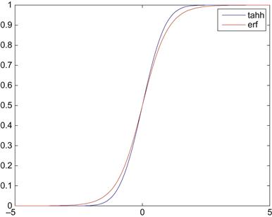
The tanh function rises more steeply towards 1 than the erf function, indicating that the response of a population with the tanh gain function has a higher level of activation for the same total input current than another population whose gain function is described by the erf function. In general, one can modify the W-C equations to allow for different sigmoidal gain functions for the two populations.
In the projects that follow, we will use yet another gain function closely related to the tanh function. Rather than rescaling and shifting the tanh function, we will multiply it by the Heaviside step function. Although there is a Heaviside step function command in MATLAB, it does not return a number if the argument is 0; so the easiest way to generate this gain function is with the following command:
Plot this function alongside the other gain functions and compare them.
34.5 Projects
In order to write our own version of pplane8, a function we’ll call nonlin_phase_plane, we are going to rely upon several already completed projects, and a new MATLAB data structure called a cell array. The general layout of our function will parallel the function phase_plane written in Chapter 14, “Introduction to Phase Plane Analysis.” A sketch of this function is shown ahead.
function stable=phase_plane(A, init)
%Determine nullclines of the linear system described by the matrix A
%Determine stability of fixed point of system which depends upon the eigenvalues of A.
%Note that for a linear system there is only one fixed at the origin.
stable=classify_fixed_pts(eigvals);
%Determine the vector fields for the phase plane
%Determine a trajectory from an initial condition using rk4 see Chapter 19, %“Voltage-Gated Ion Channels
trajectory=rk4(necessary input arguments);
%Plot everything including nullclines, vector field (using the quiver command), and the trajectory.
Updating this code to be able to handle nonlinear systems such as the W-C system requires several modifications, which we will now consider. The first part of phase_plane determines the nullclines based on the matrix A. In the nonlinear case, the nullclines are described by the curves where the derivatives are zero, so for the general nonlinear system

The x- and y-nullclines are the curves defined by f=0 and g=0, respectively. In order to make our nonlin_phase_plane generic enough to handle different nonlinear systems, we will employ the feval command and a function handle to call upon another function to determine the nullclines. Since the nullclines are no longer linear, they may intersect never, once, or more than once, producing a variable number of fixed points. Therefore, unlike in the linear case, nonlin_phase_plane will also have to determine where the nullclines intersect, and potentially analyze the stability of multiple fixed points.
Another crucial difference in analyzing the stability of fixed points for nonlinear systems is that the Jacobian of the system must be determined and evaluated at each fixed point in order to classify its stability (for a refresher, see Chapter 15, “Exploring the Fitzhugh-Nagumo Model”). Since different nonlinear systems will have different Jacobians, another function handle will be needed here. Depending upon how you write your code, there may be more function handles needed to keep nonlin_phase_plane generic enough to handle multiple nonlinear systems.
Obviously, these various function handles must be passed into nonlin_phase_plane as input arguments, but in order to keep the total number of input arguments to nonlin_phase_plane at a minimum, we can create a cell array input where each element of the array is a function handle. Cell arrays are MATLAB’s way of grouping dissimilar data structures such as character strings of different lengths or certain data types such as function handles. Working with cell arrays is similar to working with arrays that hold other data types, except that the syntax for cell arrays uses the curly bracket symbols instead of the square bracket ones. For instance, the following line of code creates a cell array with four elements, each a function handle:
You can also construct a cell array by using the cell command. The syntax would be as follows:
Accessing the first element of the cell array for use with the feval command would look something like this:
A general sketch of the code for nonlin_phase_plane is shown below. Feel free to use it as a guide when writing your own phase plane analysis code.
function [x0, y0, net_act]=nonlin_phase_plane(system_file, params, init, t, x, y)
%function [x0, y0, net_act]=nonlin_phase_plane(system_file, params, init, t, x, y)
%1) system_file is a cell array where each element of the array is a function
%handle. The first function handle calls a function for plotting the
%nullclines of the system. The second calls a function to determine the
%Jacobian of the system. The third calls a function containing the differential
%equations that define the system and are used to determine the vector
%field of the phase plane. The last function handle calls a function to
%control plotting the system. Example,
%system_file={@WCnullclines, @calculate_Jacobian, @WC_determ, @WC_plot};
%2) params contains all parameters needed by the system. Example for WC system,
%params= [W_EE, W_EI, W_IE, W_II, h_E, h_I, alpha];
%3) init contains the initial condition of the system for calculating
%4) Contains the time interval that the trajectory should be simulated for.
%5&6) The last two arguments specify the spacing of the vector fields on the
%phase plane in the x and y-directions. Example,
%Determine nullclines for the system
[Enull, Inull, vec]=feval(system_file{1}, params);
%Find fixed points where nullclines intersect.
[x0,y0]=intersections(vec,Enull,Inull,vec);
%Determine the stability of the fixed points by calculating
%the Jacobian and evaluating it at each fixed point.
%Returns the Jacobian, J, evaluated at the k-th fixed point
J=feval(system_file{2}, x0(k), y0(k), params);
%Find eigenvalues and eigenvectors of Jacobian
%Classify fixed point based on eigenvalues of J
stable{k}=classify_fxd_point(eigvals);
%Determine the vector field for the phase plane.
%Determine x and y component of vector field
sol=feval(system_file{3}, point, params);
%Find trajectories and plot them.
%Use 4th order Runge-Kutta to simulate system.
net_act=rk4(system_file{3}, init, params, t);
%Handle details of plotting the phase plane for the particular system in
feval(system_file{4}, vec, Enull, Inull, x0, y0, stable, X, Y, u, v, net_act, t);
1. Use the sketch above while writing the necessary supporting functions to create your own version of pplane8.
2. Create functions to handle the W-C system nullclines, Jacobians, and vector fields. Study the phase plane under the following conditions:
For all three parameter sets we will fix α=0.1, and the initial condition will be (Eo, Io)=(0.1, 0).
a. W_EE=W_IE=0.5, W_EI=W_II=0.3, h_E=h_I=0.001.
b. W_EE=W_IE=W_II=1, W_EI=1.6, h_E=0.325, h_I=0.175.
c. W_EE=W_IE=W_EI=1.2, W_II=0.8, h_E=0.1, h_I=0.001.
What type of fixed points do each of these parameter sets exhibit? Based on these findings is it possible that synaptic plasticity could drive a population of neurons to produce periodic activity in the population average?
3. Create the system files necessary for the F-N model studied in Chapter 15, “Exploring the Fitzhugh-Nagumo Model,” and compare results to those obtained with pplane8.