CHAPTER 7

THE EFFECTS BY THE NUMBERS

The Syndrome and Measures of National Outcome

I think the issue of gender relations within the family…actually relates to the core of power in society at a broader level. Since the family is the basic unit of society, only if there is justice and democracy within the family can you possibly have justice and democracy in the wider society.

—Ziba Mir-Hosseini

Our goal in this chapter is to assess the relationship between national outcomes and the Patrilineal/Fraternal Syndrome through regression analysis. We comprehensively surveyed outcome variables related to each of the nine dimensions of national stability, security, and resilience we assert are harmed by the Syndrome—that is, Political Stability and Governance, Security and Conflict, Economic Performance, Economic Rentierism, Health and Well-Being, Demographic Security, Education of the Population, Social Progress, and Environmental Protection (described in chapters 4–6). To foreshadow the results presented in this chapter, we echo international relations scholar Rose McDermott’s comment about the analysis she conducted on one of the Syndrome components, polygyny: “The findings are clear, consistent, and statistically robust across the board. In fact, the results are the kind of thing most social scientists strive for but almost never find in the course of their careers.”¹

Our analysis raises important questions for the academic fields of international relations and security studies, especially in light of the fact that the U.S. Department of Defense (DoD) paid for this research to be conducted. DoD’s investment has yielded a bumper crop of important findings; the question remains whether the academic and policy fields of national security studies are prepared to receive and act on them.2

Before laying out our results for each of these nine dimensions of national outcomes, we first discuss the question of causal inference from our regression analysis.

A Note on Causal Inference

Because of the lack of available panel data on the Patrilineal/Fraternal Syndrome, this is a cross-sectional analysis, and some readers might rightfully raise the issues of causality or causal directionality. We remind readers that this stage of our research is still in the exploratory phase. Because of the nature of the statistical methods used, we do not make any causal claims regarding the Syndrome and our dependent variables at present from our statistical analyses, only claims of association. We have, however, identified four reasons to anticipate that further research will advance such claims. First, given the results to be presented in this chapter, we are heartened by the remarkably consistent findings of high significance for the Syndrome in well over one hundred model runs as well as the Syndrome’s consistently substantial effect sizes. Second, these consistent, significant, strong findings are buttressed by our extensive theoretical framework for directionality (outlined in part I). Third, we offered process-tracing exploration of the pathways linking the Syndrome with worse national outcomes that also speak to the issue of causal direction (chapters 4–6). Fourth, we found, as it were, dose-dependent effects when comparing Post-Syndrome, Transition, and Syndrome societies, finding that amelioration of some of the Syndrome components also offered significant amelioration of national outcomes (discussed in chapter 9). In the future, as we and others develop longitudinal data showing the progression and regression of Syndrome symptoms and the resulting effects on national outcomes, such data developments will enable the use of causal inference analysis, thus allowing for greater confidence in assessing both causality and causal direction.

Before delving into the details of our regression analysis, a discussion of the contextual variables that modulate the effects of the Syndrome on national outcomes must be engaged. That is, the effects of the Syndrome may be dampened or exacerbated depending on the context in which they are operating in a particular nation-state at a particular time. The identification of such contextual variables then allows for specification of control variables for use in the full regression model.

Contextual Variables and Control Variables

In any empirical investigation, it is important to consider contextual variables in creating a useful empirical model. In studying the Syndrome described in this volume, we have come to the conclusion that several important contextual variables affect the degree to which the Syndrome can self-replicate, as well as the specific course it may take in a given society. We introduced one of those variables in chapter 2—that is, whether women’s labor is valuable in agriculture. Two paths diverge from that pivot point: (1) brideprice/polygyny and (2) dowry/sex ratio alteration variants. These paths do not change the overall effect of the Syndrome, but rather they mold its expression, such as whether sex ratios tend to be normal or abnormal.³

With specific reference to national outcomes, we identified at least four contextual variables that are important to our analysis. Before diving into details of the empirical investigation in the next section, we offer a short note on these contextual variables and their intersection with the Syndrome and its effects.

The first contextual variable of importance is a society’s degree of urbanization. Patrilines are easiest to cultivate in cases in which physical assets such as land or livestock represent the major source of wealth in the society. When land or livestock are no longer as important, when factors such as higher real estate prices in cities mitigate against extended household coresidence, and when women are more integrated into the formal labor force as a result of urbanization, the character of the Syndrome changes. The government may still be based on male kin alliances, but the expression of the full range of Syndrome phenomena will be constrained.⁴ In an urbanized environment, the state has become more of a real, centralized force. Monica Das Gupta perceptively comments that “modern states seek to bring all citizens directly under their rule, and to be the sole source of formal power, including for policing and military defense. This makes them likely to want to undermine traditional organizations with these powers, and clans and lineages are prime examples of independent power bases with considerable potential strength.”⁵

Das Gupta also mentions that the urban environment makes other changes in the Syndrome components easier to effect, such as female inheritance. She comments,

It is far easier to give daughters a share of assets acquired on one’s own, and non-farm occupations offer a high potential for acquiring such assets. It is also far easier for women to demand their rightful inheritance in urban areas, where legal resources are close at hand—in contrast to rural areas, where such amenities are distant and instead the woman is surrounded by lineage members hostile to the idea of property passing out of their lineage.⁶

In addition, more secularized norms may develop in urbanized populations, which may dampen the drive for sons. For example, many urbanized families in China no longer place an emphasis on the “incense and fire” funerary rituals that require sons for their performance. In addition, formal labor force participation by women is likely to be higher in urban settings than in rural settings, which may ameliorate the economic prostration of women to a certain extent, as we see in historian Mary Hartman’s analysis of northwestern Europe’s evolution in the Middle Ages (discussed more fully in chapter 8).⁷ Thus, in any empirical investigation of our theoretical framework, we include degree of urbanization as a control variable that mediates the relationship between the Syndrome and the dependent variables we wish to investigate. The precise variable we use is Percent Urban Population, 2015, from the World Bank.

The second contextual variable of importance is whether the society provides a pension system for its elderly. Patrilines retain their visceral relevance even now in the absence of such pensions, as every household must ensure that care for the elderly is provided from within its ranks. Patrilocality ensures that sons (and their wives) will typically stay on-site to provide physical care, and the brideprice fetched for one’s daughter may provide enough assets not only for the sons’ marriages but also to assist with eldercare obligations. Louisa Chiang notes, “The bridal price in many cases is seen as a retirement fund for the parents of the bride.”⁸

When a pension system is created, the relative values of sons versus daughters may change, even fairly swiftly, as has been seen in South Korea over the past quarter century.⁹ We take up this discussion in part III.

Furthermore, the effects of pension provision may synergize with those of urbanization, helping to break this association between sons and eldercare as well. Das Gupta notes: “The greater physical mobility of urban industrialized life means that whether people live near their parents is determined by their jobs and personal circumstances, not by their gender.”¹⁰ It is also true, however, that declining birth rates may undercut the feasibility of adequate pension provision during the time period in which the proportion of seniors begins to overwhelm the proportion of the working-age population needed to support them. Transition countries such as South Korea are feeling this precise pinch.¹¹ Right at the historical moment when certain Transition countries might be expected to begin to provide meaningful pension schemes, plummeting fertility may make such initiatives impossible.

Unfortunately for our empirical investigation, extant variables capturing pension coverage would overly constrain our N size. Thus, we did not include an indicator of pensions as a control variable in our multivariate models. We do, however, probe in ancillary analysis both the Syndrome’s relationship to pension coverage (in the Social Progress dimension section of this chapter), as well as the specific relationship between pension coverage and sex ratios for that subset of countries for which we have sufficient data (presented in chapter 9).

The third contextual variable of importance in mediating the effects of the Syndrome is the availability and accessibility of mass media that would allow subnational actors or even the government to promulgate new ideas concerning gender equality. Even in cases in which those messages are not always welcome, they are still heard by women and men, girls and boys, alike, perhaps planting the seeds for change.¹² Das Gupta notes that in both China and India, state-supported mass media that positively portrayed women’s empowerment has had a demonstrated positive impact on changing attitudes about gender equality and family size in those countries.¹³ Given that the rate of access to the Internet is highly correlated with urbanization (.716, p < .001), we feel we cannot include this contextual variable separately in the model, but given this high a correlation, urbanization in a sense will serve a proxy for it.

Finally, the fourth contextual variable of importance in understanding Syndrome dynamics is the presence of “shocks” to the society, such as natural disasters, climate change, invasion, and so forth, any of which may profoundly affect the expression of the Syndrome—typically intensifying it.¹⁴ For example, we have noted how polygyny rates, prostitution, rates of child marriage, and dowry deaths have all increased as a result of the devastating drought in India.¹⁵ In times of instability and fear, Syndrome societies deepen their dependence on the patrilineal/fraternal alliance for security. One of the explanations for why the number of countries with abnormal childhood sex ratios favoring males has expanded rapidly since the end of the Cold War lies, as we have seen, in a growing sense of insecurity and threat for many nations. This feeling of insecurity may thrust societies back on a system of security viewed as dependable—or at least more dependable—than the central government, leading to a resurgence of the Patrilineal/Fraternal Syndrome.¹⁶ Das Gupta notes, “The aversion to raising daughters…is driven by the fact that girls are seen as a drain on household resources. This is why the proportion “missing” rises when households face a resource crunch—such as the privations of war, a famine, or fertility decline in which total family size drops more quickly than the number of sons desired.”¹⁷

New York Times journalist Steven Erlanger’s analysis of the resurgence of the clans in the Gaza Strip is instructive in this regard.18 Given the pullout of Israeli troops, the split between the Palestinian Authority and Hamas, the high birth rate in Gaza, and the tightening economic sanctions, the sense of exigency is very high. Erlanger comments, “The disintegration of the Palestinian Authority, masked to some degree while Arafat was alive, has meant the reversion of Gazans to seek protection and identity in premodern loyalties and affiliations: the hamulla—the clan or tribe—and the mosque.”¹⁹ Erlanger quotes Gazan legislator Ziad Abu Amr as saying,

The Palestinian Authority couldn’t fulfill its role in ensuring social transformation. It had no vision for state and society-building, so it had to rely on these traditional clan structures to consolidate its role…[In the second intifada] the Palestinian Authority began to disintegrate, and its law and order structures began to disintegrate, and people found protection in parochial affiliations of region, tribe and family…. When people have to choose between faction and family, they usually choose family, and why? Because the only solid entity in Palestinian society is the family. The Palestinian Authority and the party can break down.²⁰

Power vacuums, then, in addition to more catastrophic events such as natural disasters and war, can lead to a renewed reliance on clans, which inevitably brings with it a greater subordination of women’s interests.

Unfortunately for our purposes, we could find no comprehensive indicator of “shock” that would encompass all the many sources of such feelings of vulnerability. The indices we did find included other types of risk, such as inadequate public infrastructure, which were not part of our conceptualization. For example, the World Risk Index from the University of Stuttgart examines poverty, nutrition, public infrastructure, governance, education, investment, and even gender equity.²¹ Furthermore, given that most risk indicators include war, we elected to retain conflict-related variables as dependent variables in the model, not as control variables. We therefore leave it to others to probe the relationship between shocks/exigency and the Syndrome when an appropriate variable measuring such shocks has been developed.

Control Variables

The foregoing discussion identified contextual factors that could suggest which control variables would be useful in creating a full regression model for our empirical analysis. Our choice of control variables for multivariate modeling was based on what was not identified as a possible ramification or effect of the Syndrome as adumbrated in chapters 4–6. The astute reader will know by this time that our conception of the effects of the Syndrome is quite broad. So, for example, our theoretical framework asserts economic prosperity will be tied to a country’s score on the Syndrome scale. (The complete Patrilineal/Fraternal Syndrome scale for all countries in our study is given in appendix I.) As a result, some variables commonly used as control variables in social science research, such as gross domestic product (GDP) per capita, will be reserved for use as dependent variables in our modeling analyses. We do conduct several ancillary analyses of robustness to investigate results when GDP per capita is included in the regression model for other outcome variables.

In the search for additional appropriate control variables beyond percent urban population, we turned to other variables that are not part of the Syndrome scale and that are not hypothesized to be effects of the Syndrome. Our other stipulation was that the bivariate correlation between any two control variables had to be less than .70 to avoid issues with phenomena such as multicollinearity, in which the explanatory or control variables are so highly correlated with one another that one of the variables can be predicted from a combination of the others.²² This is a problem because one of the regression assumptions is that the predictor variables should be independent; otherwise, problems with model fit and interpretation of the results occur. Furthermore, the variance inflation factors (VIFs), which quantify the severity of multicollinearity, had to be low; all VIFs for our models using these control variables in conjunction with the Syndrome ranged from 1.065 to 1.294, allowing for the retention of all the following variables in the model.²³ The variables chosen to serve as control variables, along with their rationale for inclusion, are as follows:

•   Percent Urban Population.²⁴ As noted earlier, urbanization can weaken the Patrilineal/Fraternal Syndrome’s hold over family members by breaking kin ties to land, which in turn undercuts patrilocal marriage. The correlation with the Syndrome is −.496 (p < .001), which is not high enough to introduce multicollinearity into our modeling efforts, especially because the VIF used as an indicator of multicollinearity, is a low 1.21. Although Percent Urban Population is partially a function of the wealth of the nation (measures of which are part of our dependent variable set for the economic performance dimension), the bivariate correlation between GDP per capita and Percent Urban Population in our dataset is high, but not overwhelming, at .662 (N = 168, p < .001), suggesting that with proper precaution, such as examining VIFs, we may use Percent Urban when modeling national wealth. Urbanization is significantly correlated with another control variable, Religious Fractionalization, but the correlation coefficient is only −.260.

•   Aggregated Civilization Identification, based on the work of Samuel Huntington.25 Some, such as Huntington, have controversially opined that it is civilizational identity that drives conflict and instability, and therefore we include an aggregated measure based on Huntington’s classification scheme as a control variable for our multivariate modeling. This regionally based variable also addresses Galton’s Problem, a known issue in cross-national research. Specifically, we have four categories of civilization: (1) if the nation belongs to the group of Western/Orthodox/Latin civilizations as identified by Huntington; (2) if majority Muslim; (3) if the nations are identified with Hindu/Sinic/Buddhist civilizations;²⁶ and (4) African countries without majority Muslim adherents. This variable will be treated as nominal/categorical in the data analysis. An analysis of variance showed that the Syndrome has a significant relationship with our Aggregated Civilization Identification variable (p < .001). Because we believe Syndrome and Civilization are conceptually different—one could theoretically see Syndrome components in any civilization given their historical near-universality—we felt it was appropriate to keep Civilization in the model. Indeed, this choice should make it more difficult for the Syndrome to emerge as significant in modeling analysis. Using a one-way analysis of variance (ANOVA) test for continuous variables and a chi-square test for the other categorical variable, we found that Civilization was not significantly correlated with the other control variables included in the analysis.

•   Colonial Heritage Status.²⁷ It is possible that a history of colonization might influence security and stability outcomes, and the presumption is that such a history might negatively affect such outcomes.²⁸ We developed a dichotomous variable coding whether or not a nation had ever been colonized, with the temporal delimitation being 1700–2017. For full information and Colonial Heritage Status scores, see appendix II, table AII.1. Colonial Heritage Status is not significantly related to the Syndrome score or any of the control variables included in the analysis (tested with two-sample t-tests for equality of means for the continuous variables and a chi-square for the other categorical variable).

•   Percent Arable Land.²⁹ The idea that terrain and land capacity have some bearing on security outcomes is longstanding, manifesting as the study of geopolitics by scholars such as Sir Halford Mackinder and Nicholas Spykman. More recently, an emphasis on the effect of hard-scrabble environments, such as mountains and deserts, on security and stability has been posited.³⁰ We therefore include in our model a measure of terrain—specifically, the percent of land that is arable (World Bank). This variable is not significantly related to the Syndrome score, nor to any of the other control variables.

•   Number of Unique Land Neighbors.³¹ Other scholars, for example Harvey Starr, have argued that the number of land neighbors a country has will influence its security and stability.³² The assumption is that the greater the number of neighbors, the less secure and less stable a nation will be. We include the count of land neighbors as given in Wikipedia. This variable is not significantly related to the Syndrome score, nor to any of the other control variables in the model.

•   Ethnic Fractionalization.33 Population heterogeneity has long been identified as a risk factor for insecurity and instability in national affairs.³⁴ Although we believe that the Syndrome and Ethnic Fractionalization are linked—that is, lineage groups cannot maintain a separate existence without Syndrome-like tactics—how ethnically, religiously, and linguistically fractionalized a particular nation is should be orthogonal to the existence of the Syndrome, and this information may provide additional insight in multivariate modeling. To that end, we used the Alesina group’s summary of ethnic, racial, and linguistic fractionalization scores for each country, which the Alesina group simply called “ethnic fractionalization.” The correlation between this (summary) ethnic fractionalization indicator and the Syndrome score is .520 (p < .001), which suggests that ethnic fractionalization is enhanced in the presence of patrilineal loyalty. This correlation, however, was not high enough to cause exclusion from the model, with the VIF calculated as only 1.29. As noted, this variable is significantly correlated with Urbanization, but the correlation coefficient is a very low −.260, which means that multicollinearity is not a problem.

•   Religious Fractionalization.³⁵ The Alesina group’s scores for Religious Fractionalization do not load on the same factor as the other fractionalization scores they developed. We therefore include the religious fractionalization score separately from the aggregated racial/ethnic/linguistic fractionalization score, noting that scholars have long linked this specific type of fractionalization to stability and security outcomes.³⁶ The Religious Fractionalization score is not significantly related to the Syndrome score, nor to the other control variables.

We now turn to the empirical investigation, in which we explore the proposition that the degree to which a nation-state encodes the Patrilineal/Fraternal Syndrome will be a significant predictor of its state-level outcomes on nine dimensions of security, stability, and resilience.

The Empirical Investigation

We undertook multivariate analysis using general linear models (GLM) and logistic regression analyses, with the purpose of discovering statistically significant relationships pertinent to our hypotheses. We adopt as our level of significance α ≤ .001, which is a strict standard for social science analysis, meaning the chance is one in one thousand of observing an outcome pattern as extreme or more extreme than what we have observed if a relationship between the explanatory factors and the outcome variable is not actually present. We use this value to guard against an inflated significance level by using a Bonferoni correction, which is one of several methods used to offset the problem of multiple analyses.

Operationalization of Variables

To trace whether the propositions put forward in chapters 4–6 have any empirical support, we must first identify variables to operationalize the concepts we have been discussing. The Syndrome scale was operationalized, coded, and validated in chapter 3 with further detail given in appendix I. We additionally note that the Syndrome score was imputed for four countries whose values were missing for some of the variables used in the Syndrome algorithm, as noted in chapter 3.³⁷ (The IRMI package in R, a statistical programming language, was used for imputation because of non-random missing ordinal data.) We also operationalized each of the control variables in the section immediately previous. The next step was to conceptualize the variables that would measure pertinent national outcomes.

We identified nine national outcome dimensions for which we would seek measurable indicators. These nine dimensions included the following:

1. Political Stability and Governance

2. Security and Conflict

3. Economic Performance

4. Economic Rentierism

5. Health and Well-Being

6. Demographic Security

7. Education of the Population

8. Social Progress

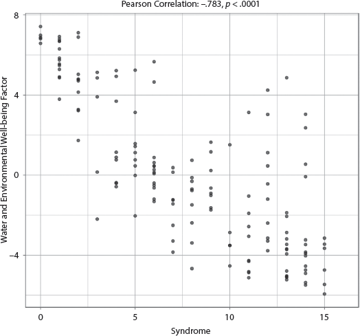
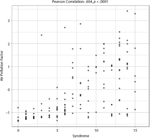
9. Environmental Protection

In general, and according to propositions elucidated in chapters 4–6, we expect to see worse outcomes in all of these nine dimensions of national security, governance, and stability the higher the score on the Syndrome scale. Our method to ascertain whether these expectations were borne out in empirical analysis was to comprehensively survey outcome variables related to each of the nine dimensions.

In searching for measurable indicators of these nine dimensions, we chose those which are commonly used in the field of International Relations and which we deemed as the most valid indicators of the dimension. In as many cases as possible, we searched for multiple indicators of the same phenomenon, or at least indicators that were fairly close in conceptualization, making it possible to avoid the issues that occur with idiosyncratic operationalizations or poor data quality for particular measures. This redundancy allows us to triangulate our results and have more confidence in the overall trends we see. Some potential variables of interest were excluded because of low N size or correlations > .9 with the other outcome variables in the list of indicators for that dimension (see the endnotes to appendix III). We also used factor analysis to further reduce the number of separate outcome variables (details are given in appendix III).

The Overall Model

After this pruning, we used each of the variables in the final list as a dependent variable in the following GLM:

Template for Reporting Results

We report our results according to the national outcome dimensions. For each dimension, we first list all the outcome variables we used in the statistical analysis, with supporting documentation provided in appendix III. Next, we provide an overall summary table for the main and ancillary analyses. The dependent variables are listed in descending order of their adjusted R-squared values. For each dependent variable, the significant explanatory variables are listed in descending order of their effect size. Then the results for each of the analyses in the summary table are discussed, and bivariate scatterplots are given for visualization purposes. For the full results tables for the models shown in the summary tables, which full results include parameter estimates, standard errors, p-values, and effect size (partial eta-squared), the reader must refer to appendix III. For ease of reference, we note the specific table number for each result as it appears in that appendix. Additionally, for models for which the Syndrome was significant, we also desired to probe the odds that a worse outcome obtains when the Syndrome is present. Therefore, we transformed the dependent variable into a binary response variable by examining histograms to obtain valid cutpoints for the logistic regression analyses (see appendix IV for full explication).

Appendix III

The full details of our methodological process for these analyses are included in appendix III. In addition to the full results tables, it also includes an alphabetical list of the variables included in the analyses, the variable name, the source from which the variable was obtained, whether the measure is nominal/ordinal/continuous, the range if applicable, the observation year(s), which directionality the variable takes, the N size, and whether any transformations were used. It also includes a link to the full replication dataset online and other pertinent material posted online.

The Nine Dimensions of National Outcomes

Dimension 1. Political Stability and Governance

In accordance with chapters 4–6, we hypothesize that nations with higher Syndrome scores will have lower levels of political stability, higher levels of corruption, lower levels of democracy and civil rights, and lower levels of government effectiveness and rule of law.

Analyses for the Political Stability and Governance Dimension

We begin our empirical data analysis with the Fragile States Index. This oft-used index measures the vulnerability of a state across a number of pressures that contribute to the risk of the state failing, becoming subject to ethnic tensions, civil war, and the inability to govern capably and transparently. We utilize two variables as ancillary analyses to test the robustness of our initial analysis. The first ancillary analysis uses our Lack of Security, Stability, and Legitimacy factor. Four indicators loaded on this factor. The first indicator is Security Apparatus, a subcomponent of the Fragile States Index, which measures the extent to which the state has a monopoly on the use of legitimate force and can guarantee the physical security of its citizens. The second indicator is State Legitimacy, also a subcomponent of the Fragile States Index, which measures the extent to which citizens believe that a given regime possesses authority or rightful power. The third indicator is the Political Instability Index, which assesses factors that destabilize governments, including the degrees of social unrest, the inability to transfer power following an election, and excessive executive control. The fourth indicator is the Global Peace Index, which measures the country’s levels of peacefulness both domestically and internationally. It also assesses societal safety and security, domestic conflict, involvement in regional or international conflict, and militarization within the state. Because the Global Peace Index is widely used, we also include it separately as our second ancillary analysis for the Fragile States Index.

Second, we use our Government System and Effectiveness factor as a main analysis. Five indicators loaded on this factor. The first indicator is the World Bank’s Government Effectiveness Index, which includes a wide range of factors that contribute to government stability and resilience. It includes institutional effectiveness; quality of basic services, such as sanitation, education, and health care; and taxation, budgeting, and financial management. The second indicator is the Functioning of Government Index, which measures the ability of government institutions in a given country to function transparently and fairly and their ability to provide needed services to citizens. The third indicator is the Democratic Political Culture Index, which looks at the norms and attitudes regarding what citizens or subjects consider right and authoritative in terms of political regimes and practices. The fourth indicator is Political System Type, which ranks regime types from authoritarian to democratic with two categories of autocracy (i.e., bounded and unbounded) and two of democracy (i.e., ineffective and effective). The fifth indicator is the Equal Protection Index, which measures equal protection under the law for minority ethnic, religious, or other groups. We used two ancillary variables as robustness checks: the World Bank Government Effectiveness Index, which is a component of the previous factor; and Regime Type, which scales political regimes from pure autocracy to minimal democracy with three categories of autocracies (i.e., pure, inclusive, and liberal).

Third, we examine corruption using the World Bank’s Corruption Index, which looks at a number of measures of transparency or corruption in state institutions. Examples include corruption among public officials, irregularity in tax collection or public contracts, bribery, and accountability.

Fourth, we look at the World Bank’s Rule of Law variable. This well-regarded indicator of the rule of law across nations measures a host of variables that range from extent of types of crime, judicial independence, and protection for private property. We use Private Property Rights in an ancillary analysis. This variable measures the extent to which a citizen may contract openly and legally for property or commercial ventures. The inability to do so demonstrates, for example, judicial ineffectiveness, power held by strong group interests, and presence of state corruption.

Fifth, we use our Lack of Freedom factor on which loaded two indicators: The Press Freedom Index, prepared by Reporters without Borders, which measures freedom of press worldwide that is a major determinant of rights and liberties within a given country; Freedom House’s Index of Political Rights, a respected project that measures democratic norms and practice worldwide by surveying competitive elections, the role of parties and interest groups, and the role of the executive.38 We used two variables for our ancillary analysis: Freedom House’s Index of Political Rights and its Civil Liberties Index. The former is a subcomponent of the larger factor. The latter surveys a nation’s respect for individual rights, including freedom of speech, press, religion, and respect for judicial process, factors that in the United States would be termed First Amendment rights, freedoms guaranteed citizens under the law.

Sixth, we take up legal and individual means to demonstrate respect and tolerance for the views of others. Freedom to Establish Religion, our main analysis, looks at a state’s openness to new expressions of freedom of conscience beyond what is traditionally accepted. For ancillary analysis, we used our Freedom of Religion and Deliberative Component factor. Two indicators loaded on this factor. The first indicator, Freedom of Religion, which guarantees freedom of conscience, is a primary measure of individual rights. The second indicator, the Deliberative Component Index, is a measure of productive dialogue within the political system. It surveys how decisions are reached in a given political system, that is, whether the system is capable of inclusive, respectful, and reasoned dialogue as opposed to coercion to accept a policy advanced by state elites.

Seventh, we look at inclusion of women in government. Our main analysis uses Percent of Seats in Parliament Held by Women, which measures the percentage of seats held by women in legislatures. We use Government Participation of Women in an ancillary analysis. This WomanStats variable looks at women in legislatures and also takes into account the number of ministerial posts held by women for that given year. (A full list of sources for all variables and models by dimension is included in appendix III.)

Model Results

We ran sixteen general linear models under the Political Stability and Governance dimension: seven of these were used in the main analysis and the other nine were used as ancillary analyses. We found that the Syndrome was significant in fifteen of these sixteen models. The only model for which the Syndrome was not significant was for the Freedom of Religion and Deliberative Component factor. Table 7.1 summarizes the GLM results of the seven main analyses and the nine ancillary analyses. We discuss the outcome variables of the seven main analysis in descending order of their R-squared values, which are indicators of the usefulness and explanatory power of the models. For each outcome variable, the significant explanatory variables are listed in descending order of effect size.

TABLE 7.1 Summary of GLM Results for the Political Stability Dimension in Descending Order of R-Squared Values

Dependent Variables	Adjusted R-squared (N)	Independent Variables (significant at .001 in descending order of effect size)
1. Fragile States Index (FSI)	.744 (172)	Syndrome Urbanization
Lack of security, stability, and legitimacy factor •   FSI’s Security Apparatus •   FSI’s State Legitimacy •   Political Instability •   Global Peace Index	.605 (158)	Syndrome Number of Land Neighbors
Global Peace Index	.365 (163)	Syndrome Number of Land Neighbors
2. Government System and Effectiveness Factor •   World Bank Government Effectiveness •   Functioning of Government •   Democratic Political Culture Index •   Political System Type •   Equal Protection Index	.565 (158)	Syndrome
World Bank Government Effectiveness	.612 (176)	Syndrome Urbanization Religious Fractionalization
Regime Type	.314 (168)	Syndrome
3. World Bank Corruption Score	.563 (176)	Syndrome Urbanization Colonial Heritage Status
4. World Bank Rule of Law Score	.561 (176)	Syndrome Urbanization Religious Fractionalization
Private Property Rights	.513 (170)	Syndrome Urbanization Colonial Heritage Status Number of Land Neighbors
5. Lack of Freedom Factor •   Press Freedom Index •   Freedom House Index of Political Rights	.415 (170)	Syndrome
Freedom House Index of Political Rights	.426 (176)	Syndrome
Civil Liberties	.459 (165)	Syndrome
6. Freedom to Establish Religion •   Freedom of Religion •   Deliberative Component Index	.245 (133)	Syndrome Terrain Ethnic Fractionalization
Freedom of Religion and Deliberative Component Factor	.276 (164)	Number of Land Neighbors
7. Percent of Seats in Parliament Held by Women	.116 (172)	Syndrome
Government Participation of Women	.221 (176)	Syndrome Muslim Civilization

Note: Ancillary analyses are in italics.

In this section, we elaborate on the GLM results of the dependent variables used in the seven main analyses. Full results for each dependent variable are available in appendix III by dimension.

1.1 Fragile States Index

(Higher scores are considered worse.)

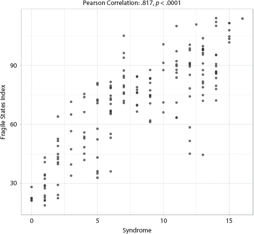
The adjusted R-squared is a remarkably strong .744, indicating that the specified model explained at least 74.4 percent of the variability of the Fragile States Index scores, and the only two variables achieving significance are the Syndrome and Percent Urban Population. See appendix III, table AIII.7.1.1, for full results. The coefficients of these two variables are opposite, that is, the higher the Syndrome score, the more fragile the state, but the higher the Urbanization percentage, the less fragile the state. The effect size for the Syndrome, however, is more than twice that of Urban Population. The bivariate correlation reveals a strong association between the Syndrome and State Fragility, with a very strong correlation of .817 (p < .0001) and a fairly tight clustering shown in the scatterplot in figure 7.1.1.

FIGURE 7.1.1 Scatterplot of Syndrome with Fragile States Index

Because the Syndrome is significant in the general linear regression model, we also ran a logistic regression model (using a binary version of the response variable). The cutoff was determined by the mean, and “worse outcome” is defined as worse than average. Details of the cutoff are included in appendix IV. The Syndrome, Urbanization, and Religious Fractionalization are the only variables that are significant in predicting the logits or predicted probabilities of a more fragile state. We specifically find that for every one unit increase in the Syndrome, the odds increase by 113 percent, or alternatively, there is a 2.13 times greater risk, that the country will experience greater fragility, after holding all other control variables constant.

We wanted to perform a robustness check on the modeling of the Fragile States Index, by adding in GDP per capita (log transformed purchasing power parity, PPP) to the model, and then as a secondary check to swap out Urbanization Rate with GDP per capita (log transformed, PPP), and see how Syndrome fares under those circumstances. That is, is wealth a more important predictor of state fragility than the Syndrome? When GDP per capita is added to the model, it renders Urbanization insignificant. Even so, the Syndrome remains significant and its effect size (.419) is larger than that of GDP per capita (.302). We also tried exchanging Urbanization with GDP per capita, and the results were very similar: the Syndrome remained significant and its effect size (.448) remained slightly larger than that of GDP per capita (.432). We find that noteworthy: whether or not women are disempowered at the household level is more important in explaining state fragility than the nation’s level of wealth.

We also used our Lack of Security, Stability, and Legitimacy factor as an ancillary analysis for the Fragile States Index. The analysis showed a remarkably strong .605 adjusted R-squared, indicating that the specified model explained at least 60.5 percent of the variability of this factor. Consistent with the results for Fragile States Index, the Syndrome is a significant predictor of the stability, peacefulness, and legitimacy of a nation. The only two variables in the model for this factor that are significant are the Syndrome and Number of Land Neighbors, but the effect size for Syndrome is almost four times larger than that of land neighbors. The coefficient for the Syndrome variable is positive, meaning that the higher the Syndrome score, the more unstable, the less peaceful, and the less legitimate the state. The coefficient for land neighbors is also positive, which means that having more neighbors predisposes a state to lower levels of stability.

We also used the Global Peace Index in an ancillary analysis for the Fragile States Index and, again, we found that Syndrome is a significant predictor of nation-state peacefulness, and in the hypothesized direction with high-Syndrome nations experiencing lower levels of peace. The analysis yielded a moderate adjusted R-squared value of .365. The other significant predictor of peacefulness was the Number of Land Neighbors. The more land neighbors a country had, the lower the level of peacefulness for the country.

1.2 Government System and Effectiveness Factor

(This factor combines several variables: World Bank Government Effectiveness, Functioning of Government, Democratic Political Culture Index, Political System Type, and Equal Protection Index. Lower scores are considered worse.)

The adjusted R-squared for this model is a strong .565, indicating that the specified model explained at least 56.5 percent of the variability of the Government System and Effectiveness factor. See appendix III, table AIII.7.1.2, for full results. Interestingly, the only significant variable in the model is the Syndrome, and the coefficient is negative, which means that the higher the Syndrome score, the lower the score on this factor. The effect size of the Syndrome is .280, much larger than the effect sizes of any other variable in the model. The bivariate correlation bears out this very strong relationship (r = −.731, p < .0001), as does the bivariate scatterplot shown in figure 7.1.2. High Syndrome scores are strongly associated with a lack of democracy and a lack of governmental effectiveness. This large N analysis corroborates our theoretical framework and suggests that the horizon for democracy and for effective governance is constrained by the presence of the Syndrome as the first political order of the society.

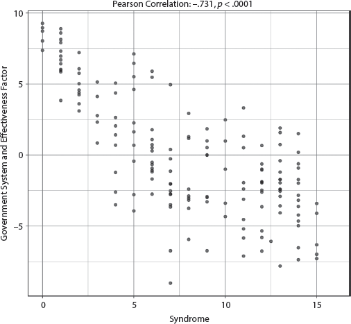
FIGURE 7.1.2 Scatterplot of Syndrome with Government System and Effectiveness Factor

Because the Syndrome is significant in the general linear regression model, we also ran a logistic regression model (using a binary version of the response variable). The Syndrome and Religious Fractionalization are the only variables that are significant in predicting the logits or predicted probabilities of more autocratic government systems and lower levels of government effectiveness. We specifically find that for every one unit increase in the Syndrome, the odds increase by 253 percent, or alternatively, the risk is 3.53 times higher that the country will experience a more autocratic governmental system and a lower level of government effectiveness, after holding all other control variables constant.

We examined the World Bank’s Government Effectiveness scale as well as a Regime Type variable as ancillary analyses for the Government System and Effectiveness factor. The first ancillary analyses showed that the model had a strong adjusted R-squared of .612 with Syndrome, Urbanization, and Religious Fractionalization as the three best predictors of government effectiveness. The negative coefficient for the Syndrome shows that higher Syndrome scores are associated with significantly lower levels of government effectiveness. The second ancillary analyses showed that the model had an adjusted R-squared of .314 for Regime Type with the Syndrome as the only significant predictor. As signified by its negative coefficient, the higher the Syndrome score, the more autocratic the nation’s regime type. Whether or not women are subordinated has significant influence on regime type and regime effectiveness.

1.3 World Bank Corruption

(Lower scores are considered worse.)

The adjusted R-squared is a strong .563, indicating that the specified model explained at least 56.3 percent of the variability of corruption, and three independent variables are statistically significant: Never Colonized, the Syndrome, and Percent Urban Population. See appendix III, table AIII.7.1.3. Although never having been colonized and having a higher percent of urban population are associated with lower levels of corruption, the Syndrome is associated with significantly higher levels of corruption. Note that the effect size for the Syndrome is the largest of the model, which is consistent with our hypotheses. The bivariate correlation is a moderately strong −.684 (p < .0001), and the scatterplot in figure 7.1.3 shows a distinctive negative slope. Corruption at the household level by means of Syndrome practices does indeed appear to be associated with corruption in the larger polity, as predicted by our theoretical framework.

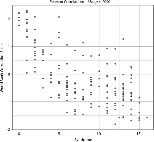
FIGURE 7.1.3 Scatterplot of Syndrome with World Bank Corruption Score

Because the Syndrome is significant in the general linear regression model, we also ran a logistic regression model (using a binary version of the response variable). The Syndrome, Urbanization, and Land Neighbors are the only variables that are significant in predicting the logits or predicted probabilities of a country experiencing high levels of corruption. We specifically find that for every one unit increase in the Syndrome, the odds increase by 23 percent, or alternatively, the risk is 1.23 times greater that the country will experience high levels of corruption, after holding all other control variables constant.

1.4 World Bank Rule of Law

(Lower scores are considered worse.)

The adjusted R-squared is a strong .561, indicating that the specified model explained at least 56.1 percent of the variability in degree of rule of law, and three variables achieve significance: the Syndrome, Percent Urban Population, and Religious Fractionalization. See appendix III, table AIII.7.1.4, for full results. Religious Fractionalization and Percent Urban Population have positive coefficients, meaning they are associated with better rule of law. The Syndrome’s coefficient is negative, however, which means the higher the Syndrome score, the more diminished the rule of law. The effect size for the Syndrome is the highest of the three significant variables, and the bivariate correlation is a moderately strong −.694 (p < .0001), with a distinctive negative slope as shown in the scatterplot in figure 7.1.4. Again, we consider this a very significant finding from a theoretical standpoint: a lack of rule of law at the household level for women is strongly and significantly associated with lack of rule of law at the level of the polity.

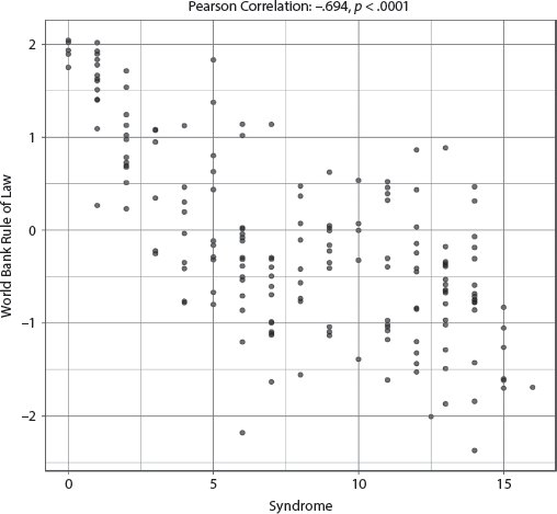
FIGURE 7.1.4 Scatterplot of Syndrome with World Bank Rule of Law Score

Because the Syndrome is significant in the general linear regression model, we also ran a logistic regression model (using a binary version of the response variable). The Syndrome, Urbanization, and Religious Fractionalization are the only variables that are significant in predicting the logits or predicted probabilities of a country experiencing a diminished rule of law. We specifically find that for every one unit increase in the Syndrome, the odds increase by 22 percent, or alternatively, the risk is 1.22 times that the country will experience a diminished rule of law, after holding all other control variables constant.

We used Private Property Rights in an ancillary analysis for the Rule of Law model and the ancillary analysis showed a strong adjusted R-squared of .513, indicating that the specified model explained at least 51.3 percent of the variability of the private property rights, and the four variables that achieve significance are Colonial Heritage Status, the Syndrome, Percent Urban Population/Urbanization, and Number of Land Neighbors. The effect size for the Syndrome is slightly larger than any of the other significant variables. The coefficients indicate that both countries that were never colonized and those with greater Urbanization are associated with greater property rights; higher scores on both the Syndrome and the Number of Land Neighbors are associated with significantly lower levels of property rights.

1.5 Lack of Freedom Factor

(This factor combines two variables: Press Freedom Index 2017 and Freedom House Index Political Rights 2016. Higher scores are considered worse.)

The adjusted R-squared is a strong .415, indicating that the specified model explained at least 41.5 percent of the variability of the Lack of Freedom factor, and the only variable in the model that was significant was the Syndrome. The coefficient for the Syndrome was positive, which means that the worse the Syndrome score, the worse the situation of political rights and press freedom in a nation. See appendix III, table AIII.7.1.5, for full results. The bivariate correlation with Syndrome was a moderately strong .625 (p < .0001), but the scatterplot in figure 7.1.5 shows quite a bit of “scatter” for middle-range Syndrome countries. So, for example, some of the countries in the central part of the graph, falling in the middle on the Syndrome scale but scoring high on this factor indicating lack of freedom, include North Korea, Cuba, and Belarus. Interestingly, these are former communist countries where the Syndrome was nominally ameliorated, at least in formal law, but nevertheless these countries still lack these political freedoms.

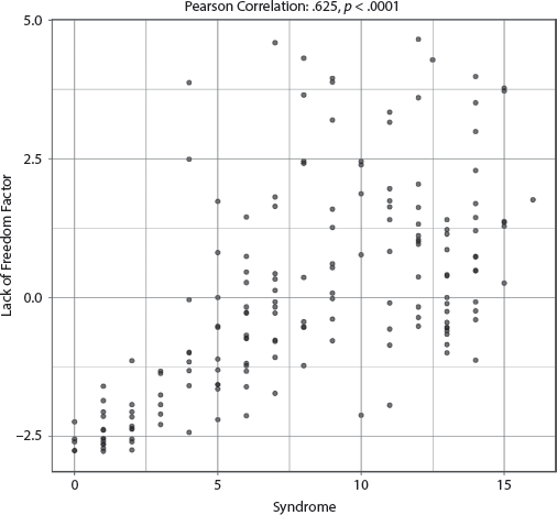
FIGURE 7.1.5 Scatterplot of Syndrome with Lack of Freedom Factor

Because the Syndrome is significant in the general linear regression model, we also ran a logistic regression model (using a binary version of the response variable). The Syndrome is the only variable that is significant in predicting the logits or predicted probabilities of low levels of press freedom and political rights. We specifically find that for every one unit increase in the Syndrome, the odds increase by 49 percent, or alternatively, the risk is 1.49 times greater that the country will experience low levels of press freedom and political rights, after holding all other control variables constant.

Note that we used Civil Liberties and Freedom House’s Index of Political Rights as ancillary variables for the Lack of Freedom Factor. The results of the former ancillary analysis also showed a strong adjusted R-squared of .459, indicating that the specified model explained at least 45.9 percent of the variability of the Civil Liberties, and the only significant variable in the model was also the Syndrome, with a noteworthy effect size. The coefficient for the Syndrome was negative, which means that higher Syndrome scores are associated with significantly lower levels of civil liberties.

The second ancillary analysis also showed a strong adjusted R-squared value of .426 and, consistent with the previous findings, the Syndrome is the only significant predictor of the political rights a country bestows on its citizens: the higher the Syndrome score, the lower the level of political rights for a country’s citizens, on average.

1.6 Freedom to Establish Religion

(Lower scores are considered worse.)

The adjusted R-squared is a moderate .245, indicating that the specified model explained at least 24.5 percent of the variability of the freedom to establish religion, and three variables in the model were significant: the Syndrome, Percent Arable Land, and Ethnic Fractionalization. See appendix III, table AIII.7.1.6, for full results. Both Percent Arable Land and Ethnic Fractionalization have positive coefficients, meaning the higher the Percent of Arable Land and the higher the Ethnic Fractionalization, the more likely it is that the nation offered the freedom to establish religion. The coefficient for the Syndrome is negative, indicating that countries with higher Syndrome scores are on average less likely to offer the freedom to establish religion. The effect sizes for the three variables are essentially the same. The bivariate correlation with Syndrome is a weak −.380, though the scatterplot in figure 7.1.6 reveals that the nations with the worst levels of freedom of religion also have higher Syndrome scores. The country in the lowest right-hand corner of the graph, with a high Syndrome score and very low Freedom to Establish Religion (the only one in the lowest category), is the United Arab Emirates.

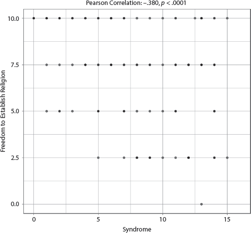
FIGURE 7.1.6 Scatterplot of Syndrome with Freedom to Establish Religion

Because the Syndrome is significant in the general linear regression model, we also ran a logistic regression model (using a binary version of the response variable). The Syndrome, Terrain, and Ethnic Fractionalization are the only variables that are significant in predicting the logits or predicted probabilities of a country having less freedom to establish religion. We specifically find that for every one unit increase in the Syndrome, the odds increase by 26 percent, or alternatively, the risk is 1.26 times greater that the country experiences less freedom to establish religion, after holding all other control variables constant.

We used our Freedom of Religion and Deliberative Component factor in an ancillary analysis, and we obtained an adjusted R-squared of .276 in the ancillary analysis. The only significant predictor of this factor is the Number of Land Neighbors.

1.7 Percent of Seats in Parliament Held by Women

(Lower scores are considered worse.)

The adjusted R-squared is a weak .116, indicating that the specified model explained only 11.6 percent of the variability of the percentage of parliament seats held by women, and the only significant variable in the model was the Syndrome. See appendix III, table AIII.7.1.7, for full results. This suggests that the percent of seats in parliament held by women may have very little to do with personal empowerment of women at the household level (as Hudson’s acquaintance who was an Afghan minister of parliament noted in the introduction). The coefficient was negative, which means the higher the Syndrome score, the lower the percentage of women in parliament. The bivariate correlation was a weak −.322 (p < .0001), with quite a bit of spread across the distribution, as shown in the scatterplot in figure 7.1.7. The outlier in the top middle of the plot is Rwanda, where the situation of women is still not very good, despite excellent levels of female representation in parliament, which we term the Rwanda Paradox.³⁹

FIGURE 7.1.7 Scatterplot of Syndrome with Percent of Seats in Parliament Held by Women

Because the Syndrome is significant in the general linear regression model, we also ran a logistic regression model (using a binary version of the response variable). Because the model does not meet the validity requirements, we do not report the results.

We also used Government Participation of Women in an ancillary analysis for Percent of Seats in Parliament held by Women. The WomanStats scale of the participation of women in government looks not only at seats in parliament, but also at women in top posts in the executive branch. The adjusted R-squared is a moderate .221, indicating that the specified model explained at least 22.1 percent of the variability of the government participation by women, again showing that government participation by women is not necessarily associated with personal empowerment of women in households. The two variables of significance in the model are the Syndrome and Muslim Civilization, each of which have a positive coefficient because higher scores on this Government Participation scale indicate worse representation of women in these government positions. The effect size for the Syndrome was almost twice that of Muslim Civilization.

Concluding Discussion for the Political Stability and Governance Dimension

For our Political Stability and Governance dimension empirical probe, we ran sixteen separate GLM analyses. Of those sixteen models, the Syndrome was significant in fifteen, was the only significant variable in six of those fifteen, and was the significant variable with the largest effect size in another eight of the analyses. Also noteworthy is that the control variables of Huntington civilization, Terrain, and Ethnic Fractionalization appear not to be overly determinative for this dimension, in contrast to a greater showing for Urbanization, Number of Land Neighbors, Religious Fractionalization, and Colonial Heritage Status.

Across the sixteen models, the findings are quite robust and consistent: the single best determinant of Political Stability overall was the Syndrome. If you wished to understand the political stability of a nation, including measures of state fragility, quality of governance, type of governance, and freedom of religion and corruption, you would derive greater explanatory power by looking at the subordination of women at the household level through the components of the Syndrome than any of the other variables examined in the model, including ethno-religious fractionalization, urbanization, colonial history, civilization, terrain, and geographic borders.

Importantly, the horizon of possibility for democracy is significantly constrained by the presence of the Syndrome, and autocracy, corruption, and lack of rule of law at the household level are strongly and significantly associated with the Syndrome at the level of the polity. That finding contradicts those of other researchers who fail to find a significant relationship between women’s empowerment and democracy, perhaps because these scholars did not use any variables in our Syndrome index that measure that empowerment at the household level.40 Our theoretical framework anticipated these relationships, and large N analysis has corroborated it.

Dimension 2. Security and Conflict

Our hypothesis is that, ceteris paribus, we expect societies with a higher Syndrome score to experience higher rates of conflict and higher rates of national and societal insecurity. We took a broad approach to this Security and Conflict dimension, looking at measures of terrorism, crime, grievance, military expenditures, internal and external conflicts, trafficking, and even a measure of women’s mobility in public spaces.

Analyses for the Security and Conflict Dimension

We begin our empirical analysis of this dimension by looking at our Violence and Stability Factor derived from factor analysis, on which loaded nine indicators. These indicators are: States of Concern to the International Community, which measures state compliance to international norms in terms of use of force, international political norms, and international economic norms; Group Grievance, a subcomponent of the Fragile States Index, which assesses the extent of cleavages between groups in society and focuses on divisions based on social or political characteristics especially those related to access to resources and services; the Political Terror Scale, which measures a country’s levels of violence and terror for a specific year; the Trafficking of Women scale, which ranks states as to laws governing trafficking of women and the degree of state compliance to that law; Intensity of Internal Conflicts, which ranks states in terms of the severity of conflict within the state; Violent Demonstrations, which ranks the frequency of violent demonstrations within a state; Political Terror, a subcomponent of the Global Peace Index, which measures a country’s levels of political terror and violence for a given year; Women’s Mobility scale, which assesses the ability of a woman to be in and to move within public spaces; and Neighboring Country Relations, a subcomponent of the Global Peace Index, which measures relations with neighboring countries on a scale from peaceful to very aggressive.

We identified six variables for ancillary analyses for the Violence and Instability factor. The first ancillary analysis used our Absence of Violent Terrorism and Freedom of Domestic Movement factor, on which loaded two indicators: Political Stability and Absence of Violence/Terrorism from the World Bank, which gauges the political instability and politically motivated violence for a given state, and Freedom of Domestic Movement, which measures the ability to move freely in a country from severely restricted to unrestricted movement. The second ancillary analysis used the World Bank’s Political Stability and Absence of Violence/Terrorism in isolation, apart from the larger factor. The third and fourth ancillary analyses used Trafficking of Women and the Political Terror Scale (both are indicators within our Violence and Instability factor, which we analyzed separately to probe more deeply into these phenomena).

Second, we look at the Societal Violence Scale, which provides data on the extent of violence within a given country in terms of scope, severity, and numbers affected.

Third, we utilize the Military Expenditures and Weapons Importation factor, on which loaded three indicators, in the main analysis. The first indicator is Military Expenditure as a percentage of GDP. This variable uses the North Atlantic Treaty Organization’s definition, which includes all expenditures labeled military, including capital expenditures, peacekeeping, personnel, pensions, social services, and maintenance figured as a percentage of a nation’s GDP. The second indicator, Military Expenditures, a subcomponent of the Global Peace Index, also measures military expenditures defined as the outlays of governments to meet costs of national armed forces, as a percentage of GDP. The third indicator in this factor, Weapons Imports, another subcomponent of the Global Peace Index, measures major conventional weapons imported for a period of time, calculated per capita, for a given country. We use Access to Weapons in an ancillary analysis. Yet another subcomponent of the Global Peace Index, this measures the ease of access to small arms and light weapons within the nation.

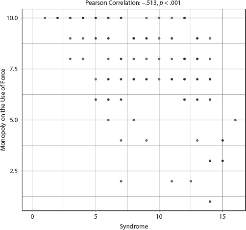
Fourth, we look at Monopoly on the Use of Force, which measures the central government’s control over weapons of force and whether that control extends to all regions of the country or is challenged by nongovernmental groups.

Fifth, we use the Global Terrorism Index, an oft-used and inclusive source that scales the impact of terrorism, including fatalities, incidents, injuries, and property damage in our main analysis. We use our Terrorism Incidents and Internal Conflict factor in the first ancillary analysis. Three indicators load on this factor: Incidents of Terrorism in a given year, a subcomponent of the Global Terrorism Index, which gives the total number of actual terrorist attacks in a given year; Internal Conflicts Fought, which measures the number and duration of a country’s internal conflicts; and the Global Terrorism Index. The second ancillary analysis used the variable Terrorism Impact, which combines terrorism injury, fatality, and property damage data. The third ancillary analysis uses the Terrorism Injury and Violent Conflict factor. Four indicators loaded on this factor: Terrorism Injuries, which scales the number injured by terrorism in a year; Terrorism Fatalities, which scales the number killed through terrorism in a given year by country; and Intensity of Violent Conflicts, which assesses the intensity of conflicts experienced by the nation-state, which are then ranked from no conflict to severe crisis; and the Overall Index of Disappearance, Conflict, and Terrorism, which includes variables such as violent conflicts, internally organized conflicts, politically motivated disappearances, battle-related deaths, and impact of armed conflict in personal freedoms. The fourth ancillary analysis uses Deaths from Internal Conflict, which is a subcomponent of the Global Peace Index.

Sixth, we examine the Perceptions of Criminality, which utilizes assessments of levels of perceived criminality in a given country, in the main analysis. We use three variables for ancillary analysis. The first is our Homicide and Violent Crime factor, on which loaded three indicators: Homicide Rates, a subcomponent of the Social Progress Index (using data from the United Nations Office on Drugs and Crime), which measures the number of homicides per one hundred thousand people; Homicide, a subcomponent of the Global Peace Index, which measures the total number of deliberate inflictions of death (penal code offences) per one hundred thousand people; and Violent Crime, which assesses whether violent crime poses significant problems for government or business. The second ancillary analysis uses Homicide, a subcomponent of the Human Freedom Index, which examines rates of intentional homicide for one hundred thousand people and then scales the data. The third ancillary analysis uses Incarceration Rate, which measures the prison population per one hundred thousand people.

Last, we look at two external conflict indicators: Deaths from External Conflict, a subcomponent of the Global Peace Index, which measures the number of deaths from conflicts external to the country analyzed, in a main analysis; and External Conflicts Fought, which measures the number and duration of conflicts outside its own territory, which a country is involved in, in an ancillary analysis.

Model Results

We ran twenty general linear model analyses under the Security and Conflict dimension; seven of these were used in the main analysis and the other thirteen were used as ancillary analyses. We found that the Syndrome was significant in fourteen of these twenty models. The six models for which the Syndrome was not significant include the following dependent variables: (1) Homicide and Violent Crime factor, (2) Homicide (Human Freedom Index, HFI), (3) Deaths from Internal Conflicts, (4) Deaths from External Conflicts, (5) External Conflicts Fought, and (6) Incarceration Rates. It is interesting that most of these aspects of the dimension are related to crime and external conflict. Table 7.2 summarizes the GLM results of the analyses for the Security and Conflict dimension. We discuss the outcome variables in descending order of the R-squared values of the explanatory model, which values are indicators of the usefulness and explanatory power of the model.

TABLE 7.2 Summary of GLM Results for the Security and Conflict Dimension in Descending Order of R-squared Values

Dependent Variable	Adjusted R-squared (N)	Independent Variables (significant at .001 in descending order of effect size)
1. Violence and Instability Factor •   States of Concern to the International Community •   Group Grievance •   Political Terror Scale •   Trafficking of Women •   Intensity of Internal Conflicts •   Violence Demonstrations •   Political Terror •   Women’s Mobility •   Relations with Neighboring Countries	.642 (145)	Syndrome Number of Land Neighbors
Absence of Violent Terrorism and Freedom of Domestic Movement Factor •   Political Stability and Absence of Violence/Terrorism •   Freedom of Domestic Movement	.525 (157)	Syndrome Number of Land Neighbors
Political Stability and Absence of Violence/Terrorism	.547 (176)	Syndrome Number of Land Neighbors
Trafficking of Women	.454 (174)	Syndrome
Political Terror Scale	.425 (163)	Syndrome Number of Land Neighbors
2. Societal Violence Scale	.377 (174)	Syndrome Number of Land Neighbors
3. Military Expenditures and Weapons Importation Factor •   Military Expenditure as Percentage of GDP •   Military Expenditures •   Weapons Imports	.318 (152)	Urbanization Syndrome
Access to Weapons	.383 (163)	Syndrome
4. Monopoly on the Use of Force	.234 (128)	Syndrome
5. Global Terrorism Index	.239 (163)	Syndrome Number of Land Neighbors
Terrorism Incidents and Internal Conflict Factor	.220 (163)	Syndrome
•   Incidents of Terrorism in a Given Year •   Internal Conflicts Fought •   Global Terrorism Index
Terrorism Impact	.213 (163)	Syndrome Number of Land Neighbors
Terrorism Injury and Violent Conflict Factor •   Terrorism Injuries •   Terrorism Fatalities •   Intensity of Violent Conflicts •   Overall Index of Disappearance, Conflict, and Terrorism	.137 (156)	Syndrome
Deaths from Internal Conflict	.135 (163)	None
6. Perceptions of Criminality	.188 (163)	Syndrome
Homicide and Violent Crime Factor •   Homicide Rates •   Homicide from Global Peace Index •   Violent Crime	.180 (154)	Syndrome
Homicide from Human Freedom Index	.110 (156)	None
Incarceration Rate	.047 (163)	None
7. External Conflicts Fought	.044 (163)	None
Deaths from External Conflict	.011 (163)	None

Note: Ancillary analyses are in italics. GDP, gross domestic product.

We elaborate on the GLM results for the seven dependent variables used in the main analysis, noting ancillary analysis results associated with each of the seven.

2.1 Violence and Instability Factor

(This factor combines several variables, including the States of Concern Scale, Group Grievance, Political Terrorism Scale, Trafficking, Internal Conflict, Violent Demonstrations, Political Terror, Women’s Mobility, and Neighboring Country Relations. Higher scores are considered worse.)

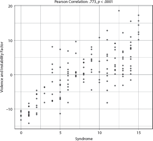
The adjusted R-squared is a remarkably strong .642, indicating that the specified model explained at least 64.2 percent of the variability of the several different measures of violence, instability, and insecurity. See appendix III, table AIII.7.2.1, for full results. Only two variables emerged as significant: the Syndrome and Number of Land Neighbors. Both variables are positively related to this factor; that is, the higher the Syndrome score or the greater the number of land neighbors, the higher the level of instability and insecurity. The effect for the Syndrome is the largest in the model, more than three times that of Land Neighbors. The bivariate relationship between the Syndrome and this factor is very strong at .773 (p < .0001), and the scatterplot in figure 7.2.1 demonstrates this well. The Syndrome is strongly and significantly associated with greater violence and instability for the nation-state.

FIGURE 7.2.1 Scatterplot of Syndrome with Violence and Instability Factor

Because the Syndrome is significant in the general linear regression model, we also ran a logistic regression model (using a binary version of the response variable). The Syndrome and Number of Land Neighbors are the only variables that are significant in predicting the logits or predicted probabilities of higher levels of violence and instability. We specifically find that for every one unit increase in the Syndrome, the odds increase by 47 percent, or alternatively, the risk is 1.47 times greater that the country experiences higher levels of violence and instability, after holding all other control variables constant.

We used four other variables in ancillary analyses as a check for the Violence and Instability factor. The first is our Absence of Violent Terrorism and Freedom of Movement factor. The adjusted R-squared for this model is a strong .525, indicating that the specified model explained at least 52.5 percent of the variability of this factor, and very much like the previous factor examined, only the Syndrome and Number of Land Neighbors were significant. This time, however, both variables are negatively associated with this factor, which means the higher the Syndrome score and the greater the Number of Land Neighbors, the lower the level of freedom of domestic movement and the more unstable, violent, and subject to terrorism is the nation-state. The effect size for the Syndrome is the strongest in the model.

The second ancillary analysis used Political Stability and Absence of Violence/Terrorism. The results showed a strong adjusted R-squared value of .547, indicating that our specified model explained at least 54.7 percent of the variability in the Political Stability and Absence of Violence/Terrorism of the countries in our study. The same two variables were significant: Syndrome and Number of Land Neighbors, with directionality as predicted. High Syndrome scores are associated with a lack of political stability and the presence of violence and terrorism.

The third ancillary analysis used Trafficking of Women. The results showed a strong adjusted R-squared value of .454, indicating that the specified model explained at least 45.4 percent of the variability of the Trafficking of Women scores, and only one variable emerges as significant: the Syndrome. The coefficient is positive, which means the higher the Syndrome score, the higher the levels of trafficking of women.

The fourth ancillary analysis used the Political Terror Scale, which yielded a strong adjusted R-squared value of .425, indicating that the specified model explained at least 42.5 percent of the variability of the Political Terror Scale scores, and two variables are significant: the Syndrome and Number of Land Neighbors, with the effect size of the former larger than that of the latter. Both variables have positive coefficients, which means the higher the Syndrome score or the greater the Number of Land Neighbors, the higher the score on the Political Terror Scale.

2.2 Societal Violence Scale

(Higher scores are considered worse.)

The adjusted R-squared is a moderate .377, indicating that the specified model explained at least 37.7 percent of the variability of the Societal Violence Scales scores, and only two variables were significant: the Syndrome and Number of Land Neighbors, with the effect size of the former being almost twice that of the latter. See appendix III, table AIII.7.2.2. The coefficients for these variables are both positive, which means the higher the Syndrome score or the greater the Number of Land Neighbors, the higher the level of societal violence. The bivariate correlation between the Syndrome and the Societal Violence Scale is moderately strong at .529 (p < .0001), and the scatterplot in figure 7.2.2 shows the distinctive trapezoidal shape we have come to recognize. The two outlier countries identified on the scatterplot with relatively high Syndrome scores but fairly low societal violence levels include Vanuatu and Brunei, two very small states.

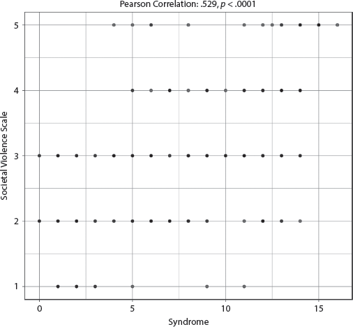
FIGURE 7.2.2 Scatterplot of Syndrome with Societal Violence Scale

Because the Syndrome is significant in the general linear regression model, we also ran a logistic regression model (using a binary version of the response variable). The Syndrome and Ethnic Fractionalization are the only variables that are significant in predicting the logits or predicted probabilities of a country scoring poorly on the Societal Violence Scale. We specifically find that for every one unit increase in the Syndrome, the odds increase by 26 percent, or alternatively, the risk is 1.26 times greater that the country scores poorly on the Societal Violence Scale, after holding all other control variables constant.

2.3 Military Expenditure and Weapons Importation Factor

(This factor combines three variables: Military Expenditure as Percentage of GDP, Military Expenditure, and Weapons Importation. Higher scores are considered worse.)

The adjusted R-squared is a moderate .318, indicating that the specified model explained at least 31.8 percent of the variability of this factor, and only two variables emerge as significant; the Syndrome and Urbanization. See appendix III, table AIII.7.2.3, for full results. Both have positive coefficients, which means the higher the Syndrome score or the higher the rate of Urbanization, the higher military expenditures and weapons imports. The finding for urbanization is somewhat intuitive, but the finding for the Syndrome is thought-provoking, especially because the effect sizes are fairly similar. The bivariate correlation between the Syndrome and this factor is weak at only .250, however, and it is not significant at the p < .001 level. The scatterplot in figure 7.2.3 reveals a considerable spread on the dependent variable across the Syndrome scores. Some countries with high expenditures and imports and also high Syndrome scores include Oman and Saudi Arabia. Israel, scoring a 6 on the Syndrome, has noticeably higher expenditures and imports than other nations at that same Syndrome level. (The United States has such a large GDP that its outsize military expenditures do not appear as a very high percentage of GDP.) Australia, scoring a 0 on the Syndrome, has a middle-range score on this outcome measure.

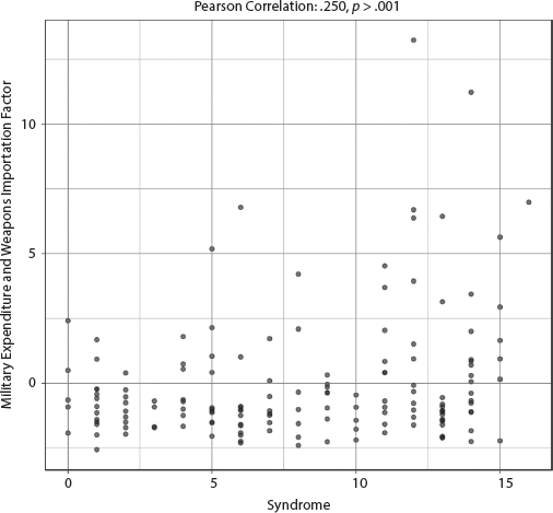
FIGURE 7.2.3 Scatterplot of Syndrome with Military Expenditures and Weapons Importation Factor

Because the Syndrome is significant in the general linear regression model, we also ran a logistic regression model (using a binary version of the response variable). Because the model does not meet the validity requirements, we do not report the results.

We also used Access to Weapons in an ancillary analysis for our Military Expenditures and Weapons Importation factor. The results show a moderately strong adjusted R-squared value of .383, indicating that the specified model explained at least 38.3 percent of the variability of access to weapons. The only significant variable in the GLM analysis is the Syndrome. Although Syndrome’s effect size is quite small, the coefficient value is in the predicted direction. We find that countries with higher Syndrome scores have higher levels of access to weapons.

2.4 Monopoly on the Use of Force

(Lower scores are considered worse, meaning that other forces or even a “deep state” compromise the state’s monopoly on the use of force.)

The adjusted R-squared is a moderate .234, indicating that the specified model explained at least 23.4 percent of the variability of monopoly on the use of force, and only one variable emerges as significant, the Syndrome, with a moderate effect size and a negative coefficient (meaning that the higher the Syndrome score, the worse the situation concerning the government’s use of force). See appendix III, table AIII.7.2.4, for full results. The bivariate correlation is a moderately strong −.513 (p < .001), with the scatterplot in figure 7.2.4 showing a clearly empty lower-left quadrant. At Syndrome scale point 7, Haiti has a very low monopoly on the use of force, and Somalia, with Syndrome scale point 14, has the worst overall score on this outcome variable.

FIGURE 7.2.4 Scatterplot of Syndrome with Monopoly on the Use of Force

Because the Syndrome is significant in the general linear regression model, we also ran a logistic regression model (using a binary version of the response variable). Because the model does not meet the validity requirements, we do not report the results.

2.5 Global Terrorism Index

(Higher scores are considered worse.)

We obtained a moderate adjusted R-squared value of .239, indicating that the specified model explained at least 23.9 percent of the variability of the Global Terrorism Index scores, and two variables emerge as significant: the Syndrome and Number of Land Neighbors. Both coefficients are positive, meaning the higher the Syndrome score and the greater the number of land neighbors, the higher the Global Terrorism score. The effect size for Syndrome is somewhat larger than that for land neighbors. See appendix III, table AIII.7.2.5. The bivariate correlation with the Syndrome is a weak .321 (p < .001), and the scatterplot in figure 7.2.5 shows that the nations with the worst scores on the Global Terrorism Index are all high-Syndrome countries, such as Iraq, Nigeria, Afghanistan, Pakistan, and Syria. At a low Syndrome score of 4, Ukraine has a high terror score, but we feel this is associated with that nation’s external conflict with Russia.

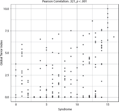
FIGURE 7.2.5 Scatterplot of Syndrome with the Global Terrorism Index

Because the Syndrome is significant in the general linear regression model, we also ran a logistic regression model (using a binary version of the response variable). Because the model does not meet the validity requirements, we do not report the results.

We used four variables in ancillary analyses as checks for the Global Terrorism Index model results. The first is Terrorism Incidents and Internal Conflict factor, which consists of Incidents of Terrorism in a given year, Internal Conflicts Fought, and the Global Terrorism Index. The adjusted R-squared for this factor is a moderate .220, indicating that the specified model explained at least 22 percent of the variability of this factor, a fairly low percentage. We note, however, that the Syndrome is the only significant variable, even though the effect size is small. The coefficient is in the expected positive direction, which means that the higher the Syndrome score, the higher the incidence of terrorism and number of internal conflicts fought.

The second variable used in ancillary analysis is Terrorism Impact. The adjusted R-squared for the GLM analysis for this dependent variable is a moderate .213, indicating that the specified model explained at least 21.3 percent of the variability of the terrorism impact ratings. The two variables that are significant are the Syndrome and the Number of Land Neighbors, each with modest effect sizes. Both coefficients are positive, meaning that the higher the Syndrome score or Number of Land Neighbors, the greater the impact of terrorism on the nation-state.

The third variable used in the analysis was the Terrorism Injury and Violent Conflict factor which combines several variables: Terrorism Injuries, Terrorism Fatalities, Intensity of Violent Conflict, and the Overall Index of Disappearance, Conflict, and Terrorism Score. The adjusted R-squared for this analysis is a weak .137, indicating that the specified model explained only at least 13.7 percent of the variability of this factor. It is noteworthy that the only significant variable in the model is the Syndrome, with the predicted negative association—that is, the higher the Syndrome score, the more affected by terrorism and internal conflict the nation, although the effect size is modest.

The fourth variable used in ancillary analysis is Deaths from Internal Conflict. The GLM results yielded a very low R-squared value of .135, and none of the independent variables in the model was significant. Given the otherwise strong relationship between the Syndrome and internal conflict, it is possible that the scale of death in any such conflict may be more dependent on internal circumstances and the nature of the adversarial groups.

2.6 Perceptions of Criminality

(Higher scores are considered worse.)

The adjusted R-squared for this variable is a weak .188, indicating that the specified model explained only at least 18.8 percent of the variability of perceptions of criminality, and the only significant variable is the Syndrome, with a modest effect size. See appendix III, table AIII.7.2.6, for full results. The coefficient is positive, which means the higher the Syndrome score, the greater the perception of criminality within the society. The bivariate association with the Syndrome is shown in the scatterplot in figure 7.2.6.

FIGURE 7.2.6 Scatterplot of Syndrome with Perceptions of Criminality

Because the Syndrome is significant in the general linear regression model, we also ran a logistic regression model (using a binary version of the response variable). Because the model does not meet the validity requirements, we do not report the results.

We used our Homicide and Violent Crime factor, as well as Homicide from the Human Freedom Index, and Incarceration Rate as ancillary analyses for this analysis. The first had a weak adjusted R-squared value of .180, indicating that the specified model explained at least 18.0 percent of the variability of the Homicide and Violent Crime factor. The Syndrome is not a significant predictor of this factor. The ancillary analyses for Homicide from the Human Freedom Index and Incarceration rate also had very low R-squared values (.110 and .047, respectively) with no significant independent variables in the models, so we do not report the results. Further investigation of this relationship is warranted, particularly given the extant literature surveyed in chapter 5 that does find an association. Crime rate variables are usually uneven in their accuracy and consistency across nations, so these low correlations may reflect those underlying data issues.

2.7 External Conflicts

(Higher scores are considered worse.)

We used two indicators of external conflicts, but the model was a poor fit for the data. The first indicator is the External Conflicts Fought scale, obtained from the Global Peace Index. It had a very low R-squared value of .044 with no significant independent variable.

The second indicator is Deaths from External Conflict, which is also a component of the Global Peace Index. The GLM results for this model yielded a low R-squared value of .011 with no significant independent variable. Because this variable cannot distinguish whether a nation is involved in an external conflict as an aggressor or as a victim, while our theoretical framework speaks primarily to aggression, this relationship will need to be probed further with more suitable variables.

Concluding Discussion for the Security and Conflict Dimension

We ran twenty analyses on numerous variables related to several aspects of the Security and Conflict dimension, such as internal conflict and violent instability, external conflict, criminal behavior, military expenditures/weapons imports/access to weapons, and terrorism. In five of these analyses, the Syndrome did not prove significant: more specifically, we found no relationship between the Syndrome and external conflict and found very little relationship between the Syndrome and criminal behavior (with the exception of the variable of Perception of Criminality). This might be an important caveat to the broader “women and peace” thesis, which suggests that as levels of gender equality rise, a nation experiences greater levels of peace and security. We note, however, that the external conflict variables used in the analysis do not capture whether the nation was the aggressor or the victim in the conflict. Further testing on the scope conditions of the relationship between the Syndrome and external conflict is needed, particularly in light of the literature reviewed in chapter 4 that does show a relationship. Furthermore, crime rate data are very uneven in quality, so again we would want to probe the relationship between the Syndrome and crime with additional variables before reaching any conclusions on the relationship.

In relation to the remaining fifteen analyses, using variables indicating internal conflict and terrorism, the Syndrome emerged as a persistently significant explanatory variable across fourteen of the fifteen models. In seven of these fifteen models, the Syndrome was the only significant variable in the model, and in seven others, it was the significant variable with the largest effect size.

Although the adjusted R-squared values ranged across the spectrum from weak to strong, and likewise for the effect sizes for the Syndrome when significant, the consistency of the findings across the model runs is noteworthy. Countries with higher Syndrome scores experience significantly greater levels of internal conflict, violent instability, and terrorism, and they are much more interested in acquiring, accessing, and importing weapons. Also noteworthy is the lack of importance of most of the other control variables, with the exception of Number of Land Neighbors.

Dimension 3. Economic Performance

We hypothesize that across a variety of measurements, nations high on the Syndrome scale should experience lower economic performance. Because we look at the character of the economic system in our Rentierism dimension, indicators related to rentierism are not examined in this discussion of the Economic Performance dimension.

Analyses for the Economic Performance Dimension

We first looked at Food Security, which measures access to sufficient and nutritious food that meets dietary standards. This index measures affordability, quality, and availability of food.

Second, we examine our Reliance on Agriculture and Lack of Prosperity factor. As the name indicates, two indicators loaded on this factor: Agriculture Value Added as Percentage of GDP and the Prosperity Index. The first indicator measures the net output of the entire agriculture sector, which includes forestry, hunting, and fishing as well as cultivation of crops and livestock production. The Prosperity Index investigates the general conditions required for prosperity, such as economic quality, business, environment, governance, security, natural environment, and health. We also separated these two variables and ran each separately as ancillary analyses.

Third, we used GDP per capita PPP (log transformed), a standard measure of income that uses a nation’s GDP for a year divided by the total population converted to international dollars and using PPP rates.

Fourth, we examined Poverty and Economic Decline. This index utilizes a number of variables, such as per capita income, GNP, unemployment, inflation, and debt to discern patterns of economic decline.

Fifth, we used our Wealth Infrastructure and Economic Freedom factor as our main analysis. Eight indicators loaded on this factor: (1) The HFI (Cato Institute) Economic Freedom Index, which presents a sweeping measure of human freedom, which it defines as the absence of coercive constraints, using seventy-nine indicators of personal and economic freedom. (2) The Index of Economic Freedom (Heritage Institute), which measures economic freedom for a country based on quantitative and qualitative factors under the headings of judicial effectiveness, government size (including spending and tax burden), regulatory efficiency, and open markets. (3) GDP per capita PPP (also analyzed separately above), which is a nation’s gross domestic product using PPP rates. (4) Property Rights, which measures the extent to which laws protect private property rights and how these laws are enforced. (5) Quality of Electrical Supply, which measures the electrical supply in terms of reliability and lack of voltage fluctuations. (6) Mobile Telephone Subscriptions, which gives the number of mobile cellular telephone subscriptions per one hundred inhabitants of a given country. (7) Internet Users, which measures the number of individuals with access to the Internet for a given country. (8) Availability of Affordable Housing, which presents survey answers to queries of satisfaction of good affordable available housing in respondent’s area. For an ancillary analysis, we used GDP Annual Growth Percentage, which measures the percent by which GDP grows or declines in a given year.

Sixth, we used the Global Competitiveness Index in a main analysis. This index addresses institutions and infrastructure that support competitiveness, human capital, markets, and capability for innovation. We used two variables in ancillary analyses: Final Consumption (log transformed), which adds the sums of expenditures by private consumption and general government consumption; and High-Technology Exports, which gives the percentage of manufactured exports in sectors with high research and development input and includes aerospace, pharmaceuticals, scientific instruments, and computer and communications technology.

Seventh, we used our Economic Inequality factor on which loaded two variables: the Gini Index and the Uneven Economic Development Index. The Gini Index is the most commonly used measurement of inequality. The Uneven Economic Development Index separates inequality within the economy from the economy’s actual performance. It notes structural inequality based on identity or class indicators and also measures opportunities for economic mobility within a given society.

Eighth, we used Female Labor Force Participation, which measures the percent of women in the total labor force.

Ninth, we used Government Expenditures as Percentage of GDP, which calculates general government spending as a share of GDP and indicates the size of government and the viability of a given state economy. It has a secondary use, which is to indicate a country’s approach to delivering public goods and services and providing social protection. For an ancillary analysis, we used Government Debt to GDP, which examines the ability of a country to make future payment on its debt given present economic data. Last, we examined in another ancillary analysis the variable Unemployment Rate, which calculates the percent of the total labor force that is unemployed but actively seeking employment.

Model Results

We ran sixteen general linear model analyses under Economic Performance and found that the Syndrome was significant in ten of those models. The six models for which the Syndrome was not significant include the following: (1) High-Technology Exports, (2) Final Consumption (log transformed), (3) Government Expenditure as Percentage of GDP, (4) Unemployment rate, (5) GDP Annual Growth Percentage, and (6) Government Debt to GDP Ratio. These results are summarized in table 7.3.

TABLE 7.3 Summary of GLM Results for the Economic Performance Dimension Ordered by Descending Adjusted R-squared Values

Dependent Variable	Adjusted R-squared (N)	Independent Variables (significant at .001 by descending order of effect size)
1. Food Security Index	.809 (113)	Syndrome Urbanization
2. Reliance on Agriculture and Lack of Prosperity Factor •   Agriculture Value Added as Percentage of GDP •   Prosperity Index	.740 (146)	Syndrome Urbanization
Prosperity Index	.746 (146)	Syndrome
		Urbanization
Agriculture, Forestry, and Fishing Value Added as Percentage of GDP	.535 (168)	Syndrome Urbanization
3. GDP per Capita PPP (log transformed)	.695 (170)	Syndrome Urbanization Muslim Civilization
4. Poverty and Economic Decline	.612 (171)	Urbanization Syndrome
5. Wealth Infrastructure and Economic Freedom Factor •   Human Freedom Index (HFI) Economic Freedom Index 2016 •   Economic Freedom Index 2017 •   GDP per Capita PPP (log transformed) •   Property Rights •   Quality of Electricity Supply •   Mobile Telephone Subscriptions •   Internet Users •   Availability of Affordable Housing	.600 (138)	Syndrome Urbanization
GDP Annual Growth Percentage	.034 (163)	None
6. Global Competitiveness Index Rankings	.564 (137)	Syndrome Urbanization
Final Consumption (log transformed)	.444 (174)	Urbanization
		Number of Land Neighbors
High Technology Exports	.156 (155)	None
7. Economic Inequality Factor •   Gini •   Uneven Economic Development Indicator	.482 (139)	Syndrome
8. Female Labor Force Participation	.471 (174)	Syndrome Urbanization Muslim Civilization Religious Fractionalization
9. Government Expenditure as Percentage of GDP	.095 (168)	None
Government Debt to GDP	.056 (168)	None
10. Unemployment Rate	.013 (174)	None

Note: The italicized variables and factors are used in ancillary analyses. GDP, gross domestic product; PPP, purchasing power parity.

3.1 Food Security Index

(Lower scores are considered worse.)

The adjusted R-squared is a remarkably strong .809, indicating that the specified model explained, impressively, at least 80.9 percent of the variability of food security. Only two variables reached significance: the Syndrome and Urbanization. See appendix III, table AIII.7.3.1, for full results. Although the effect size of Urbanization is much larger than that of the Syndrome, their effects are in the opposite direction. Higher rates of Urbanization are associated with higher levels of Food Security; higher scores on the Syndrome are associated with significantly lower levels of Food Security. The bivariate correlation (−.750, p < .0001) is very strong, and again the scatterplot in figure 7.3.1 shows the characteristic pattern of an empty lower-left quadrant and considerable spread in the right half of the graph, although most scores anchor the negative association.

FIGURE 7.3.1 Scatterplot of Syndrome with the Food Security Index

Because the Syndrome is significant in the general linear regression model, we also ran a logistic regression model (using a binary version of the response variable). Because the model does not meet the validity requirements, we do not report the results.

3.2 Reliance on Agriculture and Lack of Prosperity Factor

(This factor combines several variables: Agriculture Value Added as Percentage of GDP and Prosperity Index. Higher scores are considered worse.)

The adjusted R-squared is a remarkably strong .740, indicating that the specified model explained at least 74 percent of the variability of this factor. For this factor, combining indicators of agriculture value added and prosperity index, once again only two variables reach significance—the Syndrome and Urbanization—and the larger effect size of the two is for the Syndrome, at .325. See appendix III, table AIII.7.3.2, for full results. The very strong bivariate correlation in the scatterplot in figure 7.3.2 (correlation = .772, p < .0001) shows a strong positive relationship between the Syndrome and reliance on agriculture and lack of prosperity.

FIGURE 7.3.2 Scatterplot of Syndrome with Reliance on Agriculture and Lack of Prosperity Factor

Because the Syndrome is significant in the general linear regression model, we also ran a logistic regression model (using a binary version of the response variable). The Syndrome and Urbanization are the only variables that are significant in predicting the logits or predicted probabilities of higher levels of reliance on agriculture and lack of prosperity. We specifically find that for every one unit increase in the Syndrome, the odds increase by 49 percent, or alternatively, this risk is 1.49 times greater that the country experiences higher levels of reliance on agriculture and lack of economic prosperity, after holding all other control variables constant.

We run two ancillary analyses, the Prosperity Index as well as Agriculture, Forestry, and Fishing Value Added as Percentage of GDP. The former had a high adjusted R-squared of .746 and the latter had an adjusted R-squared of .535. Both had the same significant independent variables as the overall factor, which were the Syndrome and Urbanization. Higher values of the Syndrome were associated with significantly lower levels of prosperity and higher levels of agriculture/forestry/fishing as percent of GDP.

3.3 GDP per Capita PPP 2017

(Log transformed; lower scores are considered worse.)

The adjusted R-squared is a remarkably strong .695, indicating that the specified model explained at least 69.5 percent of the variability of GDP per capita PPP. Three variables reach significance: Muslim-Majority Countries, the Syndrome, and Urbanization. See appendix III, table AIII.7.3.3, for full results. Although Muslim-majority nations and urbanized nations have higher GDP per capita, countries with high Syndrome scores have significantly lower GDP per capita. (Because several Muslim-majority nations are also arguably rentier states, look to the Rentierism dimension for further analysis.) Although the effect size for Urbanization is almost twice that of Syndrome, the Syndrome’s effect size is more than twice that of Muslim-majority nations. We can see in the moderately strong bivariate correlation in the scatterplot in figure 7.3.3 (r = −.651, p < .0001) the same large and empty lower-left quadrant, whereas the right half of the graph, although anchoring the negative correlation, sees greater spread.

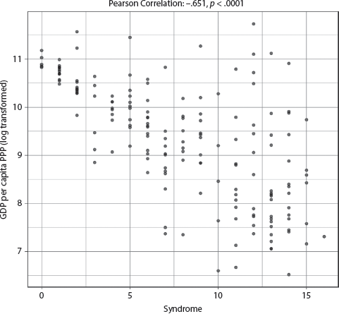
FIGURE 7.3.3 Scatterplot of Syndrome with GDP per Capita PPP 2017

Because the Syndrome is significant in the general linear regression model, we also ran a logistic regression model (using a binary version of the response variable). The Syndrome, Urbanization, and Muslim Civilization are the only variables that are significant in predicting the logits or predicted probabilities of higher GDP per capita PPP. We specifically find that for every one unit increase in the Syndrome, the odds increase by 31 percent, or alternatively, the risk is 1.31 times greater that the country experiences a lower GDP PPP, after holding all other control variables constant.

Indeed, because GDP per capita PPP (log transformed) and urbanization are correlated (with a strong bivariate correlation of .749 (p < .0001)⁴¹, which does make sense because manufactured goods have favorable terms of trade compared with commodities, it might be interesting to see the results of the same multivariate model but excluding urbanization as one of the explanatory variables. When that model is analyzed, the R-squared is diminished to .528, but the effect size of the Syndrome more than doubles, becoming the most predictive variable in the model compared with the other three significant variables (Muslim-Majority Nations and now also Never Colonized Status and Terrain (indicated by percentage of arable land)). The effect size for the Syndrome is now more than triple that of the next largest effect size variable. We also ran the logistic regression model also excluding Urbanization (using a binary version of the response variable) and find that for every one unit increase in the Syndrome, the odds increase by 50 percent, or alternatively, the risk is 1.5 times greater that the country experiences lower GDP per capita, after holding all other control variables (except Urbanization) constant.

3.4 Poverty and Economic Decline

(Higher scores are considered worse.)

The adjusted R-squared is a remarkably strong .612, indicating that the specified model explained at least 61.2 percent of the variability of poverty and economic decline, with only two out of the eight variables appearing significant: the Syndrome and Urbanization. See appendix III, table AIII.7.3.4, for full results. Although Urbanization’s effect size is slightly larger than the Syndrome, they are fairly close. Additionally, we find that the coefficient for the Syndrome is positive, indicating that countries with higher Syndrome scores have higher levels of poverty and economic decline on average. In the bivariate correlation between the Syndrome and Poverty and Economic Decline, we find a clear, positive, moderately strong relationship, with a correlation value of .650 (p < .0001). The scatterplot in figure 7.3.4 shows this relationship.

FIGURE 7.3.4 Scatterplot of Syndrome with Poverty and Economic Decline

Because the Syndrome is significant in the general linear regression model, we also ran a logistic regression model (using a binary version of the response variable). The Syndrome, Urbanization, and Muslim Civilization are the only variables that are significant in predicting the logits or predicted probabilities of higher levels of poverty and economic decline. We specifically find that for every one unit increase in the Syndrome, the odds increase by 40 percent, or alternatively, the risk is 1.4 times greater that the country experiences higher levels of poverty and economic decline, after holding all other control variables constant.

3.5 Wealth Infrastructure and Economic Freedom Factor

(This factor combines several variables: HFI Economic Freedom Index 2016, Economic Freedom Index 2017, GDP PPP (log transformed), Property Rights, Quality of Electricity Supply, Mobile Telephone Subscriptions, Internet Users, and Availability of Affordable Housing. Lower scores are considered worse.)

The adjusted R-squared is a remarkably strong .600, indicating that the specified model explained at least 60 percent of the variability of this factor. The only two variables significantly associated with measures of economic freedom, property rights, and electricity and Internet access were Urbanization and the Syndrome. High-Syndrome countries had significantly worse scores than low-Syndrome countries, and the effect size for the Syndrome is actually somewhat greater than that for Urbanization. See appendix III, table AIII.7.3.5, for full results. In the scatterplot in figure 7.3.5 for the moderately strong bivariate correlation between this factor and the Syndrome (r = −.657, p < .0001), we see a marked negative slope to the line, with virtually no countries in the lower-left quadrant of the graph. Some of the countries that appear relatively high in their wealth infrastructure and economic freedom given their high Syndrome values include, predictably, the United Arab Emirates, Qatar, and Bahrain.

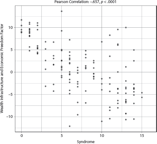
FIGURE 7.3.5 Scatterplot of Syndrome with Wealth Infrastructure and Economic Freedom Factor

Because the Syndrome is significant in the general linear regression model, we also ran a logistic regression model (using a binary version of the response variable). The Syndrome, Urbanization, and Muslim Civilization are the only variables that are significant in predicting the logits or predicted probabilities of lower levels of Wealth Infrastructure and Economic Freedom. We specifically find that for every one unit increase in the Syndrome, the odds increase by 55 percent, or alternatively, the risk is 1.55 times greater that the country experiences lower levels of Wealth Infrastructure and Economic Freedom, after holding all other control variables constant.

An ancillary analysis was run using GDP annual growth percentage. The adjusted R-squared value was a very low .034 with no significant independent variable appearing.

3.6 Global Competitiveness Index Rankings

(Higher scores are considered worse.)

The adjusted R-squared is a strong .564, indicating that the specified model explained at least 56.4 percent of the variability of the Global Competitiveness Index rankings. The only two significant variables in the model are, once again, the Syndrome and Urbanization. See appendix III, table AIII.7.3.6, for full results. Higher Urbanization is associated with higher economic competitiveness, and higher Syndrome scores are associated with lower economic competitiveness (because higher scores are worse in the ranking system for the index). The scatterplot in figure 7.3.6 shows a fairly diffuse, moderately strong bivariate relationship (r = .607, p < .0001), but with a noticeable positive trend.

FIGURE 7.3.6 Scatterplot of Syndrome with Global Competitiveness Index

Because the Syndrome is significant in the general linear regression model, we also ran a logistic regression model (using a binary version of the response variable). The Syndrome and Urbanization are the only variables that are significant in predicting the logits or predicted probabilities of worse Global Competitiveness Index rankings. We specifically find that for every one unit increase in the Syndrome, the odds increase by 26 percent, or alternatively, the risk is 1.26 times greater that the country ranks worse on the Global Competitiveness Index, after holding all other control variables constant.

We used two ancillary variables in this main analysis of Global Competitiveness Index. Final consumption (log transformed) had an adjusted R-squared of .444 with Urbanization and Land Neighbors as the only significant predictors of Global Competitiveness Index. High-technology exports had an R-squared value of .156 and no significant predictors. Because the Syndrome is not significant in these findings, we do not report the GLM results.

3.7 Economic Inequality Factor

(This factor combines two variables: the Gini Index and Uneven Economic Development. Higher scores are considered worse.)

The adjusted R-squared is a strong .482, indicating that the specified model explained at least 48.2 percent of the variability of this factor. The only variable that is significant in this model is the Syndrome. See appendix III, table AIII.7.3.7, for full results. We find a positive coefficient, indicating that on average as the Syndrome score increases (worsens), so too does a country’s economic inequality. This is consistent with our hypotheses (i.e., that a tolerance for inequality originates in the first political order). The scatterplot in figure 7.3.7 shows the clear and moderately strong positive relationship between the Syndrome and economic inequality (r = .616, p < .0001).

FIGURE 7.3.7 Scatterplot of Syndrome with Economic Inequality Factor

Because the Syndrome is significant in the general linear regression model, we also ran a logistic regression model (using a binary version of the response variable). Because the model does not meet the validity requirements, we do not report the results.

3.8 Female Labor Force Participation

(Lower scores are considered worse.)

The adjusted R-squared is a strong .471, indicating that the specified model explained at least 47.1 percent of the variability of Female Labor Force Participation, and the variables that reached significance include Muslim majority, the Syndrome, Urbanization, and Religious Fractionalization. See appendix III, table AIII.7.3.8, for full results. Muslim-majority nations and nations with high Syndrome scores have significantly lower female labor force participation; countries with higher levels of Religious Fractionalization also experience lower female labor force participation. The effect size for the Syndrome, however, dwarfs that of the other significant variables. This is explored in the bivariate scatterplot in figure 7.3.8, in which we can see a large empty lower-left quadrant (moderately strong correlation of −.414, p < .0001). On the right-hand side of the graph, however, we see no empty quadrant at all, suggesting that high-Syndrome countries range from very high to very low female labor force participation. This suggests that those viewing female labor force participation as critical to women’s empowerment may need to rethink that proposition.

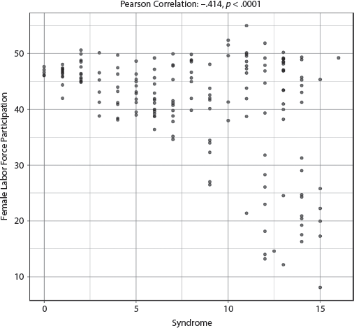
FIGURE 7.3.8 Scatterplot of Syndrome with Female Labor Force Participation

Because the Syndrome is significant in the general linear regression model, we also ran a logistic regression model (using a binary version of the response variable). Because the model does not meet the validity requirements, we do not report the results.

3.9 Government Expenditure as Percentage of GDP and Unemployment Rate

(Lower scores are considered worse for government expenditure; higher scores are considered worse for the unemployment rate.)

Because the GLM results for these two analyses in the economic performance dimension had very low adjusted R-squared values (.095 and .013, respectively) and the Syndrome was not significant in either analysis, we do not report the details of the analyses. There is a small set of wealthy nations in cultures that highly subordinate women, which may explain the negative results for the first variable. Furthermore, unemployment rates, like many rate variables, are often inconsistent and unreliable across nations. We would want to inquire further about this relationship before making any conclusions.

Concluding Discussion for the Economic Performance Dimension

Overall, we see that in ten of the sixteen analyses conducted on indicators of Economic Performance, the Syndrome showed significance—in one of the models, Economic Inequality, it was the only significant variable, and in another eight, it held the largest effect size in the model. We find the Syndrome to be highly useful in explaining a set of variables representing Wealth Infrastructure and Economic Freedom, a set of variables representing Reliance on Agriculture and Lack of Prosperity, and a set of variables representing Poverty and Economic Decline. It was the only significant variable in the model explaining Income Inequality, which is highly noteworthy given our theoretical framework, and it was also a significant variable in models of Female Labor Force Participation and Global Competitiveness. Also important, Food Security was strongly determined by Syndrome score, with nations scoring high (worse) on the Syndrome having the lowest levels of food security. The analysis for GDP (PPP) is also worth considering. Many have suggested that poor countries treat women worse, but is it possible that nations that treat women worse wind up poorer? The only control variable that added to the explanatory power of the models was Urbanization, and to a lesser degree, Civilization. In sum, countries with high Syndrome scores are simply less wealthy, more economically unequal, less competitive, less food secure, and less economically secure than nations with low Syndrome scores.

Dimension 4. Economic Rentierism

We hypothesize that countries with higher Syndrome scores will be associated with rent-based economies because the first rents are typically exacted from women. We also hypothesize that the ability of the state to concentrate assets in the hands of the government through an economy that foregrounds extraction rather than production may reflect characteristics associated with the Syndrome. In addition, the “resource curse” has been identified as being associated with higher levels of gender inequality.42 The variables that exist to tap into this concept are highly imperfect measures; we identify fuel, ore, tourism, and aid rents as possible sources of state control of rents. There is no good overall measure of rentierism, and we hope others will be able to probe this relationship with better tools than currently available.

Analyses for the Rentierism Dimension

We examine the six different variables in the rentierism dimension separately, so a factor analysis is not performed for these variables. The main outcome variable used is Total Natural Resources Rents as Percentage of GDP: Rentier states may derive a large part of national revenues from extraction and sale of resources rather than by production of goods and provision of services in country. Rentier economies are generally not highly diversified, although some states, like Russia, while well diversified, receive a large share of the state budget from the oil and gas sector. These states may have policies of very low or no taxation of citizens and pay for state services from rent profits. This has the potential to concentrate power in the hands of state elites. We then analyze the other five variables beginning with Ores and Metals Exports and Fuel Experts. These two variables account for a large percentage of some states’ economies and small sectors of others. They measure the extent of rents for these resources as the foundation of a state’s economy. Natural Resource Depletion measures the loss of a given resource, such as minerals, fishing, and fossil fuels. The variables Aid per Capita GDP and Tourism as a Percentage of GDP present alternative sectors of a state’s economy in which rentierism may be present. Whether by currency transfers for tourism or by grants of funds from bilateral and multilateral organizations, state income comes from outside sources, not local production. These two variables may have a moderate impact on a given economy, but generally they help ameliorate economic challenges rather than supply a large share of the state budget.

Model Results

We ran six general linear models under Economic Rentierism and found that the Syndrome was significant in only one of those models. The five models for which the Syndrome was not significant include (1) Ores and Metals Exports, (2) Fuel Exports, (3) Natural Resource Depletion, (4) Aid per Capita GDP, and (5) Tourism as a Percentage of GDP. Table 7.4 summarizes the results of these GLM analyses.

TABLE 7.4 Summary of GLM Results for the Rentierism Dimension in Descending Order of R-squared Values

Dependent Variable	Adjusted R-squared (N)	Independent Variables (significant at .001 by descending order of effect size)
Natural Resources as Percentage of GDP	.303 (173)	Syndrome
Fuel Exports	.250 (158)	Urbanization
Natural Resource Depletion	.243 (164)	Terrain
Tourism as a Percentage of GDP	.158 (160)	Number of Land Neighbors
Ores and Metals Exports	.061 (159)	None
Aid per Capita GDP	.024 (130)	None

Note: GDP, gross domestic product.

We elaborate on the one model for which the Syndrome was significant.

4.1 Natural Resources as a Percentage of GDP

(Higher scores are considered worse.)

The adjusted R-squared is a moderate .303, indicating that the specified model explained at least 30.3 percent of the variability of natural resources as a percentage of GDP, demonstrating moderate explanatory power for the model. See appendix III, table AIII.7.4.1, for full results. Only one variable was significant in the model (the Syndrome), although the effect size is modest. The bivariate correlation was a moderately strong .496, significant at the p ≤ .001 level. The scatterplot in figure 7.4.1 shows that those with highest levels of natural resources as a percentage of GDP all tend to have high Syndrome scores. The upper-left quadrant of the scatterplot is empty.

FIGURE 7.4.1 Scatterplot of Syndrome with Natural Resources as a Percentage of GDP

Because the Syndrome is significant in the general linear regression model, we also ran a logistic regression model (using a binary version of the response variable). The Syndrome, Terrain, and Ethnic Fractionalization are the only variables that are significant in predicting the logits or predicted probabilities of higher levels of natural resources rents as a percentage of GDP. We specifically find that for every one unit increase in the Syndrome, the odds increase by 18 percent, or alternatively, the risk is 1.18 times greater that the country experiences higher levels of natural resources rents as a percentage of GDP, after holding all other control variables constant. Although the ancillary analyses show no significant results, it is noteworthy that the most comprehensive variable among the outcome indicators is that used in the main analysis and that model did demonstrate the Syndrome’s significance.

Concluding Discussion for the Rentierism Dimension

We were interested in exploring measures of the Rentierism dimension because the structures of state economic productivity may be related to its social structures. Our empirical analysis demonstrates that existing measures of the state’s ability to extract resource-based rents are not well explained by any of the variables in the overall model tested. Only the more comprehensive variable of Natural Resources as a Percentage of GDP showed any significant correlation to the Syndrome, with the bivariate scatterplot showing that a higher percentage of these rents are significantly associated with higher Syndrome scores. In multivariate modeling, the effect size was modest; however, the Syndrome emerged as the only significant variable. The control variables Urbanization, Terrain, and Number of Land Neighbors help explain some of the ancillary rentierism outcome variables. This putative relationship between the Syndrome and rentierism deserves greater study, using better, more comprehensive indicators of rentierism once these are developed. The existing variables examine only subsets of sources of rents, which makes straightforward testing of our hypothesis difficult.

Dimension 5. Health and Well-Being

We hypothesize that nations with higher Syndrome scores will have lower levels of health and life expectancy for women, men, and children, including vulnerability to various illnesses; lower levels of spending on health; less prenatal care; higher birth rates; higher rates of habits detrimental to health; less access to clean water and sanitary facilities; undernourishment, greater hunger, and less adequate diet; and greater prevalence of female genital mutilation.

Analyses for the Health and Well-Being Dimension

We present ten separate analyses for the Health and Well-Being dimension. The first analysis includes five variables. We first examine the Healthcare Access Factor, on which three variables loaded: Access to Improved Sanitation Facilities measures the percent of the population with improved methods of sanitation. Percent of Births Attended by Skilled Staff measures the percentage of deliveries that trained personnel supervise during pregnancy, labor, and the postpartum period. This includes the training to conduct deliveries on their own and care for newborns. The third variable that loaded on this factor, Life Expectancy, measures the average number of years that a newborn, male or female, could live given death rates that apply both to their year of birth and their given locale. We also include two variables for ancillary analysis: The Sustainable Society Index combines a number of variables related to human well-being, including nutrition, improved water, sanitation, education, life expectancy, gender equality, income distribution, rates of population growth, and good governance. The final variable, Percent of Pregnant Women Receiving Prenatal Care, measures the percentage of women attended at least once by trained health workers because of her pregnancy.

The second analysis looks at national health expenditures. The main analysis variable is Health Expenditure Per Capita, which is a state’s total health expenditure per capita figured in PPP. The ancillary variable, Health Expenditure as a Percentage of GDP, includes the sum of public and private health expenditures (e.g., insurance, government funds, external borrowings and grants) calculated against a state’s GDP. It includes a large range of health services, preventive and curative, family planning activities, nutrition activities, and emergency aid.

The third analysis utilizes the Preventable Death factor as its primary analysis and applies seven variables as ancillary analyses. Four variables loaded on this factor: Lifetime Risk of Maternal Death assesses the risk of a reproductive-age woman dying from a cause related to childbearing. Infant Mortality Rate gives the number of children dying before reaching one year of age, per one thousand live births in a given year and locale. Births per One Thousand Women Ages Fifteen to Nineteen is also called the adolescent fertility rate; it calculates the births (per one thousand) by women in that age group. The final variable that loaded on this factor is Difference Between Female and Male Life Expectancy, which measures the difference between male and female life expectancy rates for a given locale. The first ancillary variable examined is Life Expectancy at Birth for Females, which gives the number of years a female newborn could live given both the age-specific death rates for the year of her birth and her locale. Maternal Mortality Rate measures a woman’s risk of death while pregnant or giving birth from any cause related to her pregnancy or childbearing, calculated per one hundred thousand live births. Deaths Due to Diarrhea of Children Under Five measures the percent of children under five years old whose deaths are due to diarrhea. The Percent of Children Under Five Who Are Stunted measures the percentage of children under five years old whose height is significantly below international standards. The Percent of Children Under Five Who Are Underweight measures the percentage of children under age five years old whose weight is significantly below international standards. Prevalence of Wasting—Percent of Children Under Five gives the percentage of children whose weight for their height is significantly below international standards. The seventh ancillary variable is Percent of Children Ages Twelve to Twenty-Three Months Immunized Against Measles. This measures the percentage of children ages twelve to twenty-three months who received at least one dose of the measles vaccination.

The fourth analysis has one variable, Total Alcohol Consumption Per Capita, which estimates the total amount of alcohol by liter consumed over a calendar year figured per capita for the population over fifteen years of age.

The fifth analysis measures three variables concerned with HIV/AIDS. The main variable analyzed is Prevalence of HIV Among Women Ages Fifteen and Over, which is women’s share of population age fifteen years old and over infected with HIV, meaning that it is the percentage of women out of the total HIV population. The first ancillary analysis uses Population Between Fifteen and Forty-Nine with HIV, measures the percentage of people ages fifteen to forty-nine years old who are infected with HIV. The second ancillary analysis uses Percentage of Adults Ages Fifteen and Forty-Nine with HIV/AIDS, measures the percentage of adults who are fifteen and forty-nine years old living with HIV/AIDS.

The sixth analysis looks at variables associated with hunger, malnutrition, and illness. We use the Global Hunger Index, which measures hunger, undernourishment, child wasting and stunting, and child mortality, in our main analysis. We use two variables in ancillary analyses. The first ancillary analysis uses our Malnutrition and Illness factor on which two indicators load: Percent of Population That Is Undernourished, which measures the percent who consume below the minimum level of dietary energy consumption continually, and Incidence of Tuberculosis per One Hundred Thousand People, which measures the estimated number of new and relapse cases of tuberculosis for one hundred thousand persons in a given year. The second ancillary analysis uses Average Dietary Energy Supply Adequacy, which assesses the adequacy of calorie intake by calculating the percentage of the Average Dietary Energy Requirement needed for dietary adequacy.

The seventh analysis has one variable, Female Genital Cutting/Mutilation, which is defined by the practice of scratching, cutting, circumcising, or stitching the external genitalia of a girl or woman. This ranges from mild forms to severe forms, such as infibulation. Type and prevalence of the practice are both examined in this variable.

The eighth analysis also has one variable, Access to Improved Water Sources, which measures the percentage of the rural population with piped water to a house or yard, or with access to a public tap, well, protected spring, or other protected water source.

The ninth analysis has one variable, Cigarette Consumption, which measures the number of cigarettes, whether machine rolled or consumer rolled, smoked per year for population over fifteen years old, figured per capita.

The tenth analysis uses the Open Defecation factor, on which load two variables: Percent of Total Population Using Open Defecation measures the percentage of population whose sanitary practices are open defecation, and Percent of Population Using Open Defecation in Urban Areas measures the percentage of population in urban areas whose sanitary practices are open defecation.

Model Results

We ran twenty-four general linear model analyses under Health and Well-Being and found that the Syndrome was significant in seventeen of those twenty-four models. The seven models for which the Syndrome was not significant include (1) Open Defecation factor, (2) Percent of Children Ages Twelve to Twenty-Three Months Immunized Against Measles, (3) Access to Improved Water, (4) Average Dietary Energy Supply Adequacy, (5) Cigarette Consumption, (6) Percent of Population Between Fifteen and Forty-Nine with HIV, and (7) Percentage of Adults Ages Fifteen and Forty-Nine with HIV/AIDS. Table 7.5 summarizes the results of the GLM analyses.

TABLE 7.5 Summary of GLM Results for the Health and Well-Being Dimension in Descending Order of R-squared Values

Dependent Variables	Adjusted R-squared (N)	Independent Variables (significant at .001 by descending order of effect size)
1. Healthcare Access Factor •   Access to Improved Sanitary Facilities •   Percentage Birth Attended by Skilled Staff •   Life Expectancy	.702 (159)	Syndrome Urbanization Muslim Civilization Ethnic Fractionalization
Sustainable Society Index Human	.715 (154)	Syndrome Well-Being Ethnic Fractionalization Muslim Civilization
Percentage of Pregnant Women	.332 (144)	Syndrome Receiving Prenatal Care Urbanization
2. Health Expenditure per Capita	.616 (168)	Syndrome Urbanization Colonial Heritage Status
Health Expenditure as Percentage of GDP	.254 (169)	Colonial Heritage Status Syndrome
3. Preventable Death Factor •   Risk of Maternal Death •   Infant Mortality Rate •   Births per One Thousand Women Ages Fifteen to Nineteen •   Difference in Life Expectancy Between Men and Women	.594 (172)	Syndrome Urbanization Ethnic Fractionalization
Life Expectancy at Birth for Females	.746 (173)	Syndrome Urbanization Muslim Civilization Ethnic Fractionalization
Maternal Mortality Rate	.699 (175)	Urbanization Syndrome Muslim Civilization Ethnic Fractionalization
Deaths Due to Diarrhea of Children Under Five	.628 (171)	Urbanization Syndrome Ethnic Fractionalization
Percentage Under Five Who Are Stunted	.550 (117)	Syndrome Syndrome
Percentage Under Five Who Are Underweight	.516 (116)	Urbanization Syndrome
Prevalence of Wasting—Percentage Under Five	.359 (116)	Urbanization Syndrome
Percentage Children Ages Twelve to Twenty-Three Months Immunized Against Measles	.209 (173)	None
4. Total Alcohol Consumption per Capita	.535 (171)	Syndrome Religious Fractionalization Terrain
5. Prevalence of HIV Among Women Ages Fifteen and Over	.525 (131)	Muslim Civilization Syndrome
Percentage of Population Between Fifteen and Forty-Nine with HIV	.243 (131)	Religious Fractionalization Western Civilization
Percentage of Adults Ages Fifteen and Forty-Nine with HIV/AIDS	.243 (130)	Religious Fractionalization Western Civilization
6. Global Hunger Index	.577 (118)	Urbanization Syndrome
Malnutrition and Illness Factor •   Percentage of Population Undernourished •   Incidence of Tuberculosis per 100,000 People	.432 (159)	Urbanization Syndrome Muslim and Western Civilizations
Average Dietary Energy Supply Adequacy	.309 (162)	Urbanization
7. Female Genital Cutting/Mutilation (FGM)	.297 (176)	Syndrome Colonial Heritage Status Ethnic Fractionalization
8. Access to Improved Water	.436 (171)	Urbanization Ethnic Fractionalization
9. Cigarette Consumption	.379 (171)	None
10. Open Defecation Factor •   Percentage of Total Population Using Open Defecation •   Percentage of Population Using Open Defecation in Urban Areas	.295 (171)	None

Note: Ancillary analysis in italics. GDP, gross domestic product.

5.1 Healthcare Access Factor

(This factor combines three variables: Access to Improved Sanitation Facilities, Percentage of Births Attended by Skilled Staff, and Life Expectancy. Lower scores are considered worse.)

The adjusted R-squared is a remarkably strong .702, indicating that the specified model explained at least 70.2 percent of the variability of this factor. Four variables proved significant: the Syndrome, Urbanization, Muslim Civilization, and Ethnic Fractionalization. See appendix III, table AIII.7.5.1, for full results. The coefficients for the Syndrome and Ethnic Fractionalization are negative, showing that the higher (worse) these two variables, the poorer the government’s ability to provide basic services to their citizens. Urbanization and Muslim Civilization were both positive meaning that the higher their score, the better health and sanitation services provided and accessed on a national basis, which also was associated with improved life expectancy. The Syndrome showed the largest effect size (.267) followed by Urbanization at .212, and Muslim Civilization at .147. Ethnic Fractionalization showed the smallest effect size out of the significant variables (.094). The bivariate correlation between Syndrome and Healthcare Access Factor is negative and very strong (r = −.707, p < .0001) as the scatterplot in figure 7.5.1 illustrates. The outliers in the lower portion of the upper-left quadrant include Mongolia, which ranks as a 3 for the Syndrome and −.02 in Healthcare Access; Haiti, which ranks as a 7 for the Syndrome and −4.14 in Healthcare Access; and Madagascar, which ranks as an 8 for the Syndrome and −4.63 in Healthcare Access.

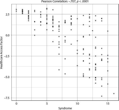
FIGURE 7.5.1 Scatterplot of Syndrome with Healthcare Access Factor

Because the Syndrome is significant in the general linear regression model, we also ran a logistic regression model (using a binary version of the response variable). The Syndrome and Urbanization are the only variables that are significant in predicting the logits or predicted probabilities of lower healthcare access for its citizens. We specifically find that for every one unit increase in the Syndrome, the odds increase by 48 percent, or alternatively, the risk is 1.48 times greater that the country experiences lower healthcare and sanitation access for its citizens, which also is associated with lower life expectancy, after accounting for the other control variables.

We used the Human Well-Being component of the Sustainable Society Index in an ancillary analysis and found a high adjusted R-squared value of .715 with Syndrome, Ethnic Fractionalization, and Muslim Civilization as the three most significant predictors of this outcome variable. Another ancillary variable used was Percentage of Pregnant Women Receiving Prenatal Care. The adjusted R-squared value was a comparatively lower .332, but the Syndrome and Urbanization were still significant predictors.

5.2 Health Expenditure per Capita

(Lower scores are considered worse.)

The adjusted R-squared is a remarkably strong .616, indicating that the specified model explained at least 61.6 percent of the variability of health expenditure per capita. Three variables are significant: Colonial Status/Never Colonized, the Syndrome, and Urbanization. See appendix III, table AIII.7.5.2, for full results. The effect size for the Syndrome was the highest, although it was only slightly higher than the effect size for Urbanization. Colonial Heritage Status/Never Colonized and Urbanization have positive coefficients that show that countries that were not colonized as well as urbanized countries have higher health expenditures per capita. The Syndrome’s negative coefficient shows that the higher the Syndrome score, the less countries spend on health care per capita, even controlling for all the other variables in the model. The bivariate correlation between Health Expenditure per Capita and the Syndrome is likewise significant and moderately strong, a negative (r = −.667, p < .0001). The scatterplot in figure 7.5.2 demonstrates a strong negative bivariate correlation with countries high on the Syndrome spending less on health. Outliers in the upper-left quadrant include the United States, which ranks 1 on Syndrome and a high $9,536 on health expenditures per capita. In the middle of the plot outliers are Japan and Singapore, which both rank as 5 on the Syndrome and spend $4,405 and $3,681, respectively, on Health Expenditure. We also find a few outliers in the lower-left quadrant: Qatar and Kuwait, both with Syndrome scores of 12; the United Arab Emirates, with a Syndrome score of 13; and Saudi Arabia, with a Syndrome score of 14.

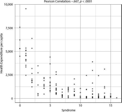
FIGURE 7.5.2 Scatterplot of Syndrome with Health Expenditure per Capita

Because the Syndrome is significant in the general linear regression model, we also ran a logistic regression model (using a binary version of the response variable). The Syndrome, Urbanization, and Religious Fractionalization are the only variables that are significant in predicting the logits or predicted probabilities of lower health expenditure per capita. We specifically find that for every one unit increase in the Syndrome, the odds increase by 70 percent, or alternatively, the risk is 1.7 times greater that the country experiences lower health expenditure per capita, after accounting for the other control variables.

We used Health Expenditure as a Percentage of GDP in an ancillary analysis but obtained a much lower adjusted R-squared value of .254. However, the Syndrome was still significant, as was Colonial Heritage Status.

5.3 Preventable Death Factor

(This factor combines four variables: Risk of Maternal Death, Infant Mortality Rate, Births per One Thousand Women Ages Fifteen to Nineteen, and Difference in Life Expectancy Between Men and Women. Higher scores are considered worse.)

The adjusted R-squared is a strong .594, indicating that the specified model explained at least 59.4 percent of the variability of this factor. Three variables are significant in this model: The Syndrome, Urbanization, and Ethnic Fractionalization. See appendix III, table AIII.7.5.3, for full results. The coefficient for the Syndrome is positive, which means that higher Syndrome countries score worse on this factor. The Ethnic Fractionalization coefficient is also positive, which means that countries that score higher in Ethnic Fractionalization score worse on this factor. The coefficient for the Urbanization variable is negative, which means that countries that are more urbanized score better on the Preventable Death factor. The effect size for Urbanization (.104) and Ethnic Fractionalization (.092) are similar, but both are smaller than that of the Syndrome (.200). The bivariate correlation between the Syndrome and the Preventable Death factor bears out this moderately strong correlation (r = .696, p = .0001) as does the scatterplot in figure 7.5.3. High Syndrome scores are associated with the variables combined in this Preventable Death factor: a higher risk of maternal death spread over the woman’s lifetime, higher mortality rates for children under five years of age, higher number of births for women ages fifteen to nineteen years old, and higher discrepancies in life expectancy between men and women. These correlations show that health for women and children is severely compromised in Syndrome countries.

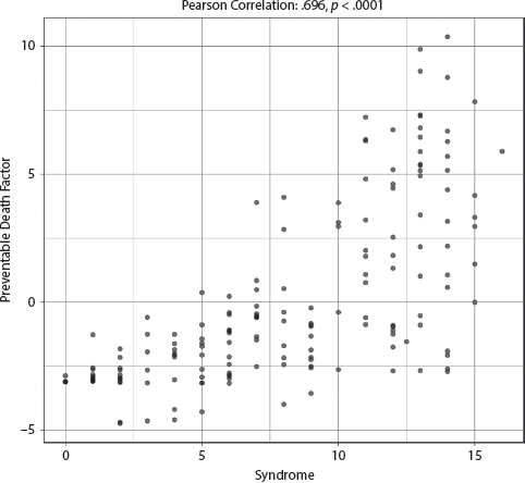
FIGURE 7.5.3 Scatterplot of Syndrome with Preventable Death Factor

Because the Syndrome is significant in the general linear regression model, we also ran a logistic regression model (using a binary version of the response variable). The Syndrome and Urbanization are the only variables that are significant in predicting the logits or predicted probabilities of high instances of preventable death. We specifically find that for every one unit increase in the Syndrome, the odds increase by 84 percent, or alternatively, the risk is 1.84 times greater that the country experiences high instances of preventable death, after accounting for the other control variables.

We used seven ancillary variables (see table 7.5) in a GLM analysis and the adjusted R-squared values ranged from .209 to .746. The Syndrome is significant in six of these ancillary analyses, including female life expectancy, maternal mortality, infant mortality, and various measures of stunting, wasting, and malnutrition in children. The only outcome variable that is not significant is percentage of children ages twelve to twenty-three months immunized against measles; this variable has also the lowest adjusted R-squared. Overall, many important health variables concerning women and children are best explained by the Syndrome.

5.4 Total Alcohol Consumption per Capita

(Higher scores are considered worse.)

The adjusted R-squared is a strong .535, indicating that the specified model explained at least 53.5 percent of the variability of total alcohol consumption per capita. Three variables are significant: the Syndrome (effect size .292), Percent of Arable Terrain (.082), and Religious Fractionalization (.086). See appendix III, table AIII.7.5.4, for full results. The coefficient for the Syndrome is negative, which means that countries that rank higher on the Syndrome consume less alcohol per capita. The other two variables are positive, which means that countries that rank high on percent of Arable Terrain and Religious Fractionalization have higher rates of alcohol consumption per capita. The bivariate correlation between the Syndrome and Alcohol Consumption is moderately strong and negative (−.655, p < .0001). The bivariate scatterplot in figure 7.5.4 also illustrates this relationship in its downward slope. Our original hypothesis was that societies with strong male kin networks may correlate with higher alcohol consumption. Research on health issues link higher alcohol consumption with increased incidence of (male) suicide and illness. These data do not support our hypothesis, and countries that score higher on the Syndrome have lower rates of alcohol consumption per capita. Many high-Syndrome countries are Muslim-majority nations and have lower availability of alcohol for consumption for religious reasons. The country on the far right ranking 15 on the Syndrome and in the middle rank on alcohol consumption is Nigeria. The country with the highest alcohol consumption is Moldova, the second-highest country is Belarus. Both rank low in Syndrome but high in Alcohol Consumption.

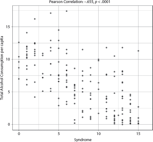
FIGURE 7.5.4 Scatterplot of Syndrome with Total Alcohol Consumption per Capita

Because the Syndrome is significant in the general linear regression model, we also ran a logistic regression model (using a binary version of the response variable). The Syndrome is the only variable that is significant in predicting the logits or predicted probabilities of higher levels of total alcohol consumption. We specifically find that for every one unit increase in the Syndrome, the odds decrease by 37 percent that the country experiences high levels of total alcohol consumption per capita, after accounting for the other control variables.

5.5 Prevalence of HIV Among Women Ages Fifteen and Over

(Higher scores are considered worse.)

The adjusted R-squared is a strong .525, indicating that the specified model explained at least 52.5 percent of the variability of prevalence of HIV among women. Two variables are significant: Muslim Civilization (CIV = 2) with an effect size of .176 and the Syndrome with an only slightly smaller effect size of .163. See appendix III, table AIII.7.5.5, for full results. The coefficient for Muslim Civilization is negative, which means that the prevalence of HIV among women over fifteen years of age is lower in Muslim-majority countries. The coefficient for the Syndrome is positive, which means that there is a higher prevalence of HIV among women age fifteen and over in higher-Syndrome-scoring countries. The bivariate correlation between the Syndrome and Prevalence of HIV Among Women Age Fifteen and Over is a moderately strong .553 (p < .0001). This is demonstrated in the upward slant of the scatterplot in figure 7.5.5.

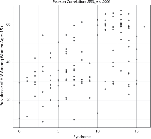
FIGURE 7.5.5 Scatterplot of Syndrome with Prevalence of HIV Among Women Ages Fifteen and Over

Because the Syndrome is significant in the general linear regression model, we also ran a logistic regression model (using a binary version of the response variable). The Syndrome is the only variable that is significant in predicting the logits or predicted probabilities of higher prevalence of HIV among women age fifteen and over. We specifically find that for every one unit increase in the Syndrome, the odds increase by 58 percent, or alternatively, the risk is 1.58 times greater that the country experiences higher prevalence of HIV among women ages fifteen and over, after holding all other control variables constant.

We use Percentage of Population Between Fifteen and Forty-Nine with HIV and Percentage of Adults Ages Fifteen to Forty-Nine with HIV/AIDS as ancillary variables. The adjusted values for these two ancillary analyses are .243 and .245, respectively. Because the Syndrome was not significant in either analysis, we do not report the results. These findings illustrate the need to use more than one variable measuring HIV burden so that a more nuanced picture of the relationship with the Syndrome can be observed.

5.6 Global Hunger Index

(Higher scores are considered worse.)

The adjusted R-squared is a strong .577, indicating that the specified model explained at least 57.7 percent of the variability of Global Hunger Index scores. The two variables that prove significant are the Syndrome (effect size .213) and Urbanization (effect size .294). See appendix III, table AIII.7.5.6, for full results. The coefficient for the Syndrome is positive and for Urbanization is negative. This means that levels of hunger are higher on average in Syndrome countries and lower in urbanized countries. The bivariate correlation between the Syndrome and the Global Hunger Index is a moderately strong .682 (p < .0001). The bivariate scatterplot in figure 7.5.6 demonstrates this relationship, showing an upward curve. We identify some of the outliers in the upper middle portion of the scatterplot: Haiti (Syndrome = 7) and Madagascar (Syndrome = 8). We also find that the Central African Republic and Chad, both with high Syndrome scores of 14, achieve the two highest (worst) values for the Global Hunger Index.

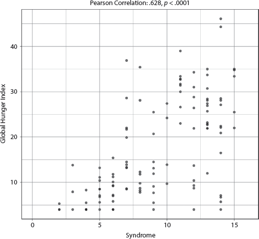
FIGURE 7.5.6 Scatterplot of Syndrome with Global Hunger Index

Because the Syndrome is significant in the general linear regression model, we also ran a logistic regression model (using a binary version of the response variable). The Syndrome and Urbanization are the only variables that are significant in predicting the logits or predicted probabilities of worse scores on the Global Hunger Index. We specifically find that for every one unit increase in the Syndrome, the odds increase by 80 percent, or alternatively, the risk is 1.8 times greater that the country experiences worse scores on the Global Hunger Index, after holding all other control variables constant.

We use our Malnutrition and Illness factor and Average Dietary Energy Supply Adequacy as ancillary variables and their adjusted R-squared values are .432 and .309 respectively. The Syndrome is a significant predictor of the former, but not of the latter. We question the results of the latter test, given the results we have seen with the Global Hunger Index, as well as the Food Security Index analyzed in a previous dimension. Overall, the Syndrome appears highly determinative of food insecurity, hunger, and malnutrition within nations.

5.7 Female Genital Cutting/Mutilation

(Higher scores are considered worse.)

The adjusted R-squared is a moderate .297, indicating that the specified model explained at least 29.7 percent of the variability of female genital cutting/mutilation. Three variables are significant in this model: Colonial Heritage Status /Never Colonized, the Syndrome, and Ethnic Fractionalization. The Syndrome has a higher effect size (.113) than does Colonial Heritage Status/Never Colonized (.088) or Ethnic Fractionalization (.082). See appendix III, table AIII.7.5.7, for full results. The bivariate correlation between the Syndrome and female genital cutting/mutilation (FGM) is moderately strong (r = .439, p < .0001). The coefficients for all three variables are positive, which shows that the higher scores on each correlate with higher use of FGM.

The positive Colonial Heritage Status/Never Colonized coefficient proves significant largely because FGM is not randomly distributed over countries as it is a civilization-specific practice. Most never-colonized nations are rated 1 on the FGM scale (i.e., the practice is rare or found in small enclaves of minority populations that practice FGM). Of the countries ranked 1, FGM is confined to enclaves. When we ran an ANOVA to test this relationship, the relationship between Colonial Heritage Status/Never Colonized with FGM was not significant.

The scatterplot in Figure 7.5.7 tells the story that only high-Syndrome countries rank higher (i.e., 2, 3, and 4) on the FGM scale. Low-Syndrome countries have no or rare prevalence of FGM. The blank upper-left quadrant on the scatterplot shows that the prevalence of FGM for countries that rank low on the Syndrome is essentially nonexistent or very rare (<11 percent) for prevalence of FGM, whereas countries with higher Syndrome scores show significant prevalence of FGM.

FIGURE 7.5.7 Scatterplot of Syndrome with Female Genital Cutting/Mutilation

Because the Syndrome is significant in the general linear regression model, we also ran a logistic regression model (using a binary version of the response variable). The Syndrome and Ethnic Fractionalization are the only variables that are significant in predicting the logits or predicted probabilities of FGM occurring (more than rarely). We specifically find that for every one unit increase in the Syndrome, the odds increase by 76 percent, or alternatively, the risk is 1.76 times greater that FGM occurs in a country, after holding all other control variables constant.

5.8 Access to Improved Water

(Lower scores are considered worse.)

We ran a GLM analysis for access to improved water and find a moderate adjusted R-squared value of .436. Because the Syndrome is not a significant predictor, we do not report the results.

5.9 Cigarette Consumption

(Higher scores are considered worse.)

The GLM analysis for cigarette consumption shows a low adjusted R-squared value of .379. Because the Syndrome is not a significant predictor, we do not report the results.

5.10 Open Defecation Factor

(This factor includes Percent Population Using Open Defecation and also Percent Population Using Open Defecation in Urban Areas. Higher scores are considered worse.)

This factor has an even lower adjusted R-squared (.295) than cigarette consumption. Because the Syndrome was not significant, we do not report the results.

Concluding Discussion for the Health and Well-Being Dimension

For our Health and Well-Being dimension’s empirical analysis, we ran twenty-four GLM analyses of health and well-being using twenty single dependent variables and four extracted factors. Syndrome was significant in three of the four factors, and for fourteen of the twenty single variables, for a total of seventeen of the twenty-four models run. The Syndrome had the largest effect size in eight of the models, showing strong predictive power not only for variables directly related to women’s health, such as female life expectancy, maternal mortality, FGM, and prevalence of HIV among women, but also child-related health indices, such as percent under age five who are stunted, wasted, or underweight, as well as population-wide indicators of hunger, illness, mortality, and levels of government investment in healthcare expenditures. Also noteworthy in explaining some of the national health outcome variables were the control variables of Urbanization, Civilization, Ethnic Fractionalization, and Colonial Heritage Status. The Syndrome, however, was by far the most consistently determinative explanatory variable. To understand issues of national health and nutrition, we need to look at Syndrome-encoding practices within the country. The subordination of women at the household level clearly undermines national health and nutrition outcomes. Our theoretical framework anticipated this relationship and our large N analysis corroborated it.

Dimension 6. Demographic Security

We hypothesize that nations manifesting a strong patrilineal/fraternal culture as measured by the Syndrome Index tend to have higher levels of demographic insecurity, to wit, higher fertility rates, lower contraceptive prevalence, higher unmet need for contraception, a larger youth bulge, and greater demographic pressures.

Analyses for the Demographic Security Dimension

We performed five main analyses for the Demographic Security dimension. First, we look at Mother’s Mean Age at First Birth, which provides data on early pregnancies before the age of eighteen, which adversely affect women’s health and future opportunities as well as raises fertility rates overall. For an ancillary analysis, we utilize Fertility Rates Ages Fifteen to Nineteen. High numbers of births among this age cohort often correlate with the practice of child marriage.

The second analysis consists of one variable, Demographic Pressure, which measures the impact of population size upon the state. On one hand, a growing population may produce pressures related to food supply, access to safe water, and the ability to provide needed infrastructure. On the other hand, insufficient population growth in various sectors of the population may lead to insufficient economic growth to support social security and pensions for aging citizens.

The third analysis consists of one variable, Total Fertility, which gives the number of children that a woman would give birth to if she were to live to the end of her childbearing years and her childbearing falls in line with the fertility rates of a specified year. Generally, it is the total number of births for a woman in her lifetime.43

The fourth analysis consisted of two variables measuring contraceptive use. Contraceptive Prevalence, our main variable, measures use of any contraceptive for women ages fifteen to forty-nine. The ancillary analysis used the variable Unmet Need for Contraception, which measures the percentage of women of reproductive age, married or in a union, who say they want to stop or delay childbearing, but who are not currently using any method of contraception.

The fifth analysis looks at the Youth Risk Factor (which is not a factor in the sense we have been using that term, but rather the name given this variable by its creators). This variable looks at the size of the seventeen- to twenty-six-year-old age cohort in ratio to the size of a country’s total labor force. High values of this variable signify a large youth bulge, which has been associated with higher levels of internal instability and violence.

Model Results

We ran seven general linear model analyses under Demographic Security and found that the Syndrome was significant in five of those seven models. The two models for which the Syndrome was not significant include (1) Fertility Rates for Females Ages Fifteen to Nineteen and (2) Unmet Need for Contraception. Note, however, that variables similar in conceptualization, such as Mother’s Age at First Birth and Contraceptive Prevalence, are significantly associated with the Syndrome. Table 7.6 summarizes the results of the GLM analyses.

TABLE 7.6 Summary of GLM Results for the Demographic Security Dimension in Descending Order of R-squared Values

Dependent Variables	Adjusted R-squared (N)	Independent Variables (significant at .001 by descending order of effect size)
1. Mother’s Mean Age at First Birth	.712 (123)	Syndrome
Fertility Rates Ages Fifteen to Nineteen	.486 (174)	Urbanization Ethnic Fractionalization
2. Demographic Pressure	.707 (172)	Syndrome Urbanization
3. Total Fertility Rate	.602 (175)	Syndrome Urbanization Ethnic Fractionalization
4. Contraceptive Prevalence	.491 (135)	Syndrome Ethnic Fractionalization
Unmet Need for Contraception	.304 (116)	None
5. Youth Risk Factor	.479 (166)	Syndrome

Note: Ancillary analysis in italics.

6.1 Mother’s Mean Age at First Birth

(Lower scores are considered worse.)

The adjusted R-squared is a remarkably strong .712, indicating that the specified model explained at least 71.2 percent of the variability of mother’s mean age at first birth. The Syndrome was the only significant predictor of this dependent variable, with the Syndrome having an effect size that was much larger than any other variable. See appendix III, table AIII.7.6.1, for full results. There is a significant negative correlation between the Syndrome and mother’s mean age at first birth (beta = −.436): the higher the Syndrome score for a country, the lower the mother’s age at first birth. This is confirmed by the scatterplot in figure 7.6.1 in which we find a very strong linear relationship between mean age of first birth and the Syndrome (r = −.818, p < .001). We find a few countries that buck this trend, including Jamaica and Mongolia, with Syndrome values of 3, which both have surprisingly low mean age at first birth, and Jordan (Syndrome = 14), which has surprisingly high mean age at first birth.

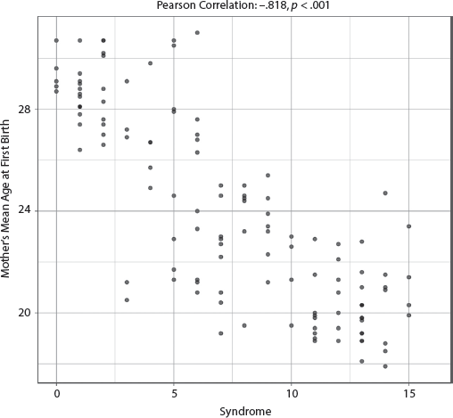
FIGURE 7.6.1 Scatterplot of Syndrome with Mother’s Mean Age at First Birth

Because the Syndrome is significant in the general linear regression model, we also ran a logistic regression model (using a binary version of the response variable). The Syndrome is the only variable that is significant in predicting the logits or predicted probabilities of lower average age of first birth for the mother. We specifically find that for every one unit increase in the Syndrome, the odds increase by 62 percent, or alternatively, the risk is 1.62 times greater that the country experiences a lower average age of first birth for the mother, after holding all other control variables constant.

We use fertility rates for ages fifteen to nineteen as a variable in an ancillary analysis, and the GLM analysis show a moderately strong adjusted R-squared value of .486. Because the Syndrome is not a significant predictor, we do not report the results. The contrast in the findings of the main and ancillary analysis are interesting and bear further scrutiny.

6.2 Demographic Pressure

(Higher scores are considered worse.)

The Fund for Peace’s Demographic Pressure variable is defined as pressures on the population, such as disease and natural disasters, which make it difficult for the government to protect its citizens or if the government demonstrates a lack of capacity or will to do so. It combines measures related to natural disasters, disease, environment, pollution, food scarcity, malnutrition, water scarcity, population growth, youth bulge, and mortality. Higher scores mean higher demographic pressure.

We regressed Demographic Pressure on our eight independent variables and found that the adjusted R-squared is a remarkably strong .707, indicating that at least 70 percent of the variability in demographic pressure can be explained by our model. The only two significant predictors in the model are the Syndrome and percent Urbanization, with the Syndrome having an effect size almost twice as large as percent Urbanization. See appendix III, table AIII.7.6.2, for full results. These findings support our claim that nations that manifest a strong patrilineal culture as measured by the Syndrome Index tend to experience higher demographic pressures. The bivariate scatterplot in figure 7.6.2 further amplifies this finding: a very strong linear correlation exists between the Syndrome and Demographic pressure (r = .793, p < .0001). We find that the Bahamas and Cape Verde have surprisingly high demographic pressure given their low Syndrome scores (2 and 3, respectively). Some of the countries with the highest Syndrome scores and the highest Demographic Pressure scores include Somalia, South Sudan, and Malawi. On the other end of the plot, countries with both the lowest Syndrome scores and lowest Demographic Pressure scores include Australia and Finland.

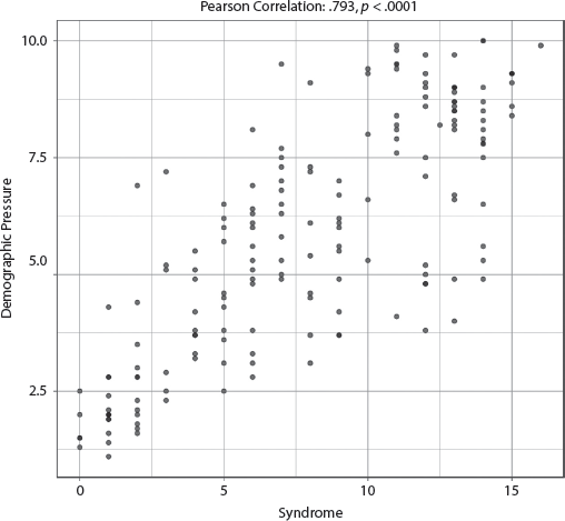
FIGURE 7.6.2 Scatterplot of Syndrome with Demographic Pressure

Because the Syndrome is significant in the general linear regression model, we also ran a logistic regression model (using a binary version of the response variable). The Syndrome and Urbanization are the only variables that are significant in predicting the logits or predicted probabilities of higher levels of demographic pressure. We specifically find that for every one unit increase in the Syndrome, the odds increase by 39 percent, or alternatively, the risk is 1.39 times greater that the country experiences higher levels of demographic pressure, after holding all other control variables constant.

6.3 Total Fertility Rate

(Higher scores are considered worse.)

The adjusted R-squared is a remarkably strong .602, indicating that the specified model explained at least 60.2 percent of the variability in total fertility rates. Three of the eight independent variables had significant explanatory power: the Syndrome, Percent Urbanization, and degree of Ethnic Fractionalization, in descending order of effect size. See appendix III, table AIII.7.6.3, for full results. The effect size of the Syndrome is twice that of either of the other two variables. The subordination of women at the household level, as represented by the Syndrome score, is critical in predicting total fertility rates, more so than Urbanization and Ethnic Fractionalization. These findings support our hypothesis that nations with strong patrilineal cultures as measured by the Syndrome Index tend to have higher fertility rates, after controlling for the effects of our control variables. The scatterplot in figure 7.6.3 confirms this finding when Syndrome is regressed alone against fertility rate: the correlation coefficient is very strong (r = .714, p < .001).

FIGURE 7.6.3 Scatterplot of Syndrome with Total Fertility Rate

We find the significance of Ethnic Fractionalization understandable; as demographer Richard Cincotta notes, “the more a state politically, economically, and socially marginalizes an ethnic group, the more likely that group is to grow demographically.”44

Because the Syndrome is significant in the general linear regression model, we also ran a logistic regression model (using a binary version of the response variable). The Syndrome, Urbanization, and Ethnic Fractionalization are the only variables that are significant in predicting the logits or predicted probabilities of higher total fertility rates. We specifically find that for every one unit increase in the Syndrome, the odds increase by 92 percent, or alternatively, the risk is 1.92 times greater that the country experiences higher total fertility rates, after holding all other control variables constant.

6.4 Contraceptive Prevalence

(Lower scores are considered worse.)

The adjusted R-squared is a strong .491, indicating that at least 49.1 percent of the variability in the prevalence of contraceptive use can be explained by the specified model and only two of the independent variables had significant explanatory powers: the Syndrome and Ethnic Fractionalization. See appendix III, table AIII.7.6.4, for full results. The Syndrome had a slightly higher effect size, .195 versus .102. This finding shows that women in nations with higher Syndrome scores have a harder time accessing contraceptive methods (beta estimate = −2.542, p < .0001) after controlling for the effects of the other covariates. Similarly, women in highly ethnically fractionalized societies face similar problems in accessing contraception. The results for the Syndrome are supported by the bivariate scatterplot in figure 7.6.4, which shows a moderately strong negative linear correlation (r = −.636, p < .0001) between Syndrome and Contraceptive Prevalence.

FIGURE 7.6.4 Scatterplot of Syndrome with Contraceptive Prevalence

Because the Syndrome is significant in the general linear regression model, we also ran a logistic regression model (using a binary version of the response variable). The Syndrome is the only variable that is significant in predicting the logits or predicted probabilities of lower percentages of women ages fifteen to forty-nine who are practicing, or whose sexual partners are practicing, any form of contraception (less than 49.42 percent). We specifically find that for every one unit increase in the Syndrome, the odds increase by 32 percent, or alternatively, the risk is 1.32 times greater that the country experiences lower contraceptive prevalence, after holding all other control variables constant.

We used Unmet Need for Contraception as an ancillary variable and the GLM analysis yielded an adjusted R-squared value of .304. Because the Syndrome was not a significant predictor, we do not report the results. It is possible that contraceptive prevalence is more tightly related to subordinative mechanisms than the operationalization of unmet need, for which responses may vary as a result of cultural norms.

6.5 Youth Risk Factor

(Higher scores are considered worse.)

The Youth Risk Factor includes variables that measure the stress that large youth cohorts exert within a given country, defined as the ratio of the seventeen- to twenty-six-year-old age cohort to the size of the laborforce. High values of this factor signify a large youth bulge, which has been associated with higher levels of internal instability and violence.45

The adjusted R-squared is a strong .479, indicating that the specified model explained at least 47.9 percent of the variability of the Youth Risk Factor or youth bulge. Of the eight independent variables, only one had significant explanatory power: the Syndrome. See appendix III, table AIII.7.6.5, for full results. The Syndrome’s effect size was much larger than any of the other variables. This finding shows that Syndrome is a good predictor of youth bulge after controlling for the effects of the other covariates. The coefficient for the Syndrome is positive, meaning the higher the Syndrome score, the greater the score on the youth risk factor or bigger youth bulge.

The scatterplot in figure 7.6.5 supports this finding when only Syndrome is compared against Youth Risk Factor, which measures the size of the youth bulge. We can see that there is a moderately strong positive and significant linear correlation (r = .699, p < .001) between these two variables: higher Syndrome scores are associated with a higher youth bulge, on average. The countries with a Syndrome score of 3 that appear to be outliers in the scatterplot are Jamaica, Cape Verde, and Mongolia, with surprisingly high youth risk factor levels given their low Syndrome score. Some of the countries with both the highest Syndrome and the highest youth risk factor levels include Syria, Jordan, Iraq, and Yemen.

FIGURE 7.6.5 Scatterplot of Syndrome with Youth Risk Factor

Because the Syndrome is significant in the general linear regression model, we also ran a logistic regression model (using a binary version of the response variable). The Syndrome and Religious Fractionalization are the only variables that are significant in predicting the logits or predicted probabilities of higher ratio of the number of seventeen- to twenty-six-year-olds to the size of the country’s total labor force. We specifically find that for every one unit increase in the Syndrome, the odds increase by 68 percent, or alternatively, the risk is 1.68 times greater that the country experiences a higher youth risk factor, after holding all other control variables constant.

Concluding Discussion for the Demographic Security Dimension

The Patrilineal/Fraternal Syndrome was a highly significant predictor of five of the seven demographic variables we analyzed, after controlling for the effects of our covariates of interest. The Syndrome also had the highest overall explanatory power as measured by effect size in these five runs. Only the control variables of Urbanization and Ethnic Fractionalization somewhat contributed to the explanatory power of the models for these national outcome variables. These findings support our hypothesis that nations manifesting a strong patrilineal culture as measured by the Syndrome Index tend to have higher fertility rates, have lower contraceptive prevalence, have a lower age at first birth for mothers, possess a larger youth bulge, and experience greater demographic pressures. Demographic insecurity is clearly related to the Patrilineal/Fraternal Syndrome as a security provision mechanism, with its low levels of women’s empowerment at the household level.

Dimension 7. Education of the Population

We hypothesize that countries with higher Syndrome scores will experience lower levels of literacy and education, both as a whole and specifically among women and girls. We also predict that high-Syndrome countries will have larger discrepancies in the education and literacy between men and women.

Analyses for the Education Dimension

The first analysis uses the variable, Average Years of Schooling, which uses the average numbers of years of education received by people age twenty-five and older as our main analysis. We also analyze two ancillary variables: the Gender Parity Index for Secondary School, which calculates the ratio of girls to boys enrolled at the secondary level in public and private schools, and the Gender Parity Index for Primary School, which does the same for primary school.

The second analysis uses one variable, Access to Basic Knowledge, a Social Progress Index subcomponent, which measures adult literacy rate, primary school enrollment, secondary school enrollment, gender parity in secondary enrollment, and access to quality education.

The third analysis has one variable, Access to Information and Communications, which measures mobile phone subscriptions, internet users, access to online governance, and access to independent media for a given country.

The fourth analysis utilizes Overall Literacy Rate of Males and Females, defined as the percent of total population age fifteen and above that can read and write a simple statement (generally numeracy is required as well) as the main analytical variable. We add one ancillary analysis, which uses our Male-Female Literacy and Education Difference Factor on which load two variables: Discrepancy in Educational Attainment Between Females and Males measures and scales the difference between male and female education level reached, and Male-Female Difference in Literacy Rates measures the difference in percent of male and female literacy rates (age twenty-five and older).

The fifth, sixth, and seventh analyses all use one variable apiece. The fifth analysis looks at the Female Literacy Rate Ages Fifteen to Twenty-Four, which is the percentage of women ages fifteen to twenty-four who can read and write simple statements and do simple arithmetic. The sixth analysis examines Survival Rate to Last Year of Primary School for Females, which measures children enrolled in first grade who eventually reach the last grade by percent. Survival figures often are quite different from enrollment figures, and so this is an important variable to include. The seventh analysis examines Government Expenditures per Student Secondary as Percentage of GDP per Capita, which gives the average general government expenditures per student in a given level of education, here secondary, as a percent of GDP per capita.

Model Results

We ran ten general linear model analyses under Education of the Population and found that the Syndrome was significant in six of those ten models. The four models for which the Syndrome was not significant include (1) the Male-Female Literacy Ratio and Discrepancy in Educational Attainment Factor, (2) the Gender Parity Index for Primary School, (3) the Gender Parity Index for Secondary School, and (4) Government Expenditures per Student Secondary as Percentage of GDP per Capita. Table 7.7 summarizes the results of these analyses.

TABLE 7.7 Summary of GLM Results for the Education Dimension in Descending Order of R-squared Values

Dependent Variables	Adjusted R-squared (N)	Independent Variables (significant at .001 by descending order of effect size)
1. Average Years of Schooling	.676 (172)	Syndrome Urbanization Religious Fractionalization Muslim Civilization
Gender Parity Index for Secondary School	.238 (163)	None
Gender Parity Index for Primary School	.110 (169)	None
2. Access to Basic Knowledge	.608 (158)	Syndrome Muslim Civilization Urbanization
3. Access to Information and Communications	.569 (168)	Urbanization Syndrome
4. Overall Literacy Rate	.555 (148)	Syndrome Urbanization Ethnic Fractionalization
Male–Female Literacy and Education Difference Factor •   Discrepancy in Educational Attainment Between Females and Males •   Male–Female Difference in Literacy Rates	.064 (124)	None
5. Female Literacy Rate Ages Fifteen to Twenty-Four	.495 (126)	Syndrome Urbanization Ethnic Fractionalization
6. Survival Rate to Last Year of Primary School for Females	.485 (150)	Muslim Civilization Urbanization Syndrome
7. Government Expenditures per Student Secondary as Percentage of GDP per Capita	.042 (129)	None

Note: Ancillary analysis in italics. GDP, gross domestic product.

7.1 Average Years of Schooling

(Lower scores are considered worse.)

The adjusted R-squared is a remarkably strong .676, indicating that the specified model explained at least 67.6 percent of the variability of average years of schooling. We find that Civilization (Muslim), Patrilineal/Fraternal Syndrome, Urbanization, and Religious Fractionalization are all significant variables in this model. See appendix III, table AIII.7.7.1, for full results. We further note that the Syndrome has by far the largest effect size—more than twice as large as any of the other significant variables. The sign of the Syndrome coefficient is in the predicted direction (negative, meaning the lower (better) the Syndrome score, the higher the average years of schooling for men and women ages twenty-five and older). It appears that the strongest determinant of average years of schooling is the Patrilineal/Fraternal Syndrome, which corroborates our hypothesis.

We further note that the direction of the coefficient for Urbanization is positive, which indicates that as the level of urbanization increases, a country’s average years of schooling improves. We find that the direction of the coefficient for Religious Fractionalization is positive, which indicates that as the fractionalization increases, a country’s average years of schooling also increases. We also find that the coefficient for Muslim civilizations is positive, which indicates that predominantly Muslim countries experience higher average years of schooling.

In further analysis, we note the bivariate correlation between the Syndrome and the Average Years of Schooling is a very strong −.754 (p < .0001), with the scatterplot in figure 7.7.1 showing this relationship. All of the lowest scores for this variable are found in the countries with the highest Syndrome scores and in the vast majority of medium-lower scores (with the exception of Cape Verde, which can be found in the lower-left quadrant, with a Syndrome Score of 3 and only 4.8 average years of schooling). Countries with the lowest (best) Syndrome scores attain the highest levels of average years of schooling.

FIGURE 7.7.1 Scatterplot of Syndrome with Average Years of Schooling

Because the Syndrome is significant in the general linear regression model, we also ran a logistic regression model (using a binary version of the response variable). The Syndrome, Urbanization, and Religious Fractionalization are the only variables that are significant in predicting the logits or predicted probabilities of average years of schooling being less than or only to the completion of primary education. We specifically find that for every one unit increase in the Syndrome, the odds increase by 57 percent, or alternatively, the risk is 1.57 times greater that the country experiences average years of schooling less than or only to the completion of primary education, after holding all other control variables constant.

We use two variables in ancillary analyses: Gender Parity Index for secondary school and Gender Parity Index for primary school. The former had a low adjusted R-squared value of .238, whereas the latter had an even lower R-squared value of .110. Because the Syndrome was not significant in either of these analyses, we do not report the details of the analyses. Parity has increased dramatically over the past two decades, and so this result is not unexpected.

7.2 Access to Basic Knowledge

(Lower scores are considered worse.)

The adjusted R-squared is a remarkably strong .608, indicating that the specified model explained at least 60.8 percent of the variability of access to basic knowledge. We find that Civilization (Muslim), Patrilineal/Fraternal Syndrome, and Urbanization are all significant variables in this model. See appendix III, table AIII.7.7.2, for full results. We further note that Syndrome has the largest effect size—more than twice as large as Muslim Civilizations or Urbanization, which also appear as significant in that model run. The sign of the Syndrome coefficient is in the predicted direction (negative, meaning the lower (better) the Syndrome score the higher the access to basic knowledge). This variable is an index that considers adult literacy rates, primary school enrollment, lower secondary school enrollment, upper secondary school enrollment, and gender parity in secondary enrollment. When a country has a worse Syndrome score, a country’s score for the combination of these knowledge assets worsens. It appears that the strongest determinant of access to basic knowledge in a society is the Patrilineal/Fraternal Syndrome, which corroborates our hypothesis.

We further note that the direction of the coefficient for Urbanization is positive, which indicates that as the level of urbanization increases, a country’s access to basic knowledge score improves. We also find that the coefficient for Muslim civilizations is positive, which indicates that predominantly Muslim countries experience greater access to basic knowledge than the comparison group.

In further analysis, we note the bivariate correlation between the Syndrome and the Access to Basic Knowledge variable is a very strong −.704 (p < .0001), with the bivariate scatterplot in figure 7.7.2 showing the relationship. Although higher scores can be found at every different level of Syndrome, all of the lowest scores for this variable are found in the countries with the highest Syndrome scores. This indicates that, although higher scores for access to basic knowledge can occur at any level, lower scores are essentially eliminated when countries have lower levels of Syndrome practices. We additionally note that the country that experiences the lowest level of access to basic knowledge is also the country that experiences the worst Syndrome score (16), South Sudan.

FIGURE 7.7.2 Scatterplot of Syndrome with Access to Basic Knowledge

Because the Syndrome is significant in the general linear regression model, we also ran a logistic regression model (using a binary version of the response variable). The Syndrome, Urbanization, and Muslim Civilization are the only variables that are significant in predicting the logits or predicted probabilities of lower access to basic knowledge. We specifically find that for every one unit increase in the Syndrome, the odds increase by 66 percent, or alternatively, the risk is 1.66 times greater that the country experiences lower access to basic knowledge, after holding all other control variables constant.

7.3 Access to Information and Communications

(Lower scores are considered worse.)

This variable is an index that considers mobile telephone subscriptions, internet users, and the Press Freedom Index. The adjusted R-squared is a strong .569, indicating that the specified model explained at least 56.9 percent of the variability of access to information and communication. We find that Patrilineal/Fraternal Syndrome and Urbanization are the only significant variables in this model. See appendix III, table AIII.7.7.3, for full results. We note that Syndrome does not have the largest effect size for this variable, but that the effect size of Urbanization is only slightly larger than Syndrome. The coefficient for Urbanization indicates that as the level of urbanization increases, the access to information and communication also increases on average. The sign of the Syndrome coefficient is also in the predicted direction (negative, meaning the lower/better the Syndrome score, the higher the access to information and communication).

In further analysis, we note the bivariate correlation between the Syndrome and the Access to Information and Communication variable is a moderately strong −.674 (p < .0001), with the scatterplot in figure 7.7.3 showing the relationship. With the exception of one outlier in the lower-left quadrant (Cuba with a Syndrome score of 4), lower scores of access are not found for countries with lower (better) Syndrome levels. Additionally, the highest access scores attained are found for countries with better Syndrome scores.

FIGURE 7.7.3 Scatterplot of Syndrome with Access to Information and Communication

Because the Syndrome is significant in the general linear regression model, we also ran a logistic regression model (using a binary version of the response variable). The Syndrome and Urbanization are the only variables that are significant in predicting the logits or predicted probabilities of lower access to information and communications. We specifically find that for every one unit increase in the Syndrome, the odds increase by 28 percent, or alternatively, the risk is 1.28 times greater that the country experiences lower access to information and communications, after holding all other control variables constant.

7.4 Overall Literacy Rate for the Fifteen and Over Population

(Lower scores are considered worse.)

The adjusted R-squared is a strong .555, indicating that the specified model explained at least 55.5 percent of the variability of overall literacy rates. We find that Patrilineal/Fraternal Syndrome, Urbanization, and Ethnic Fractionalization are all significant variables in this model. See appendix III, table AIII.7.7.4, for full results. We note that the Syndrome has the largest effect size in this model, more than twice as large as Ethnic Fractionalization and almost twice as large as Urbanization. The sign of the Syndrome coefficient is in the predicted direction (negative, meaning the worse the Syndrome score, the lower the overall literacy of men and women in a country). It appears that the strongest determinant of the overall literacy in the adult population is the Patrilineal/Fraternal Syndrome, which corroborates our hypothesis.

We additionally note that coefficients indicate that countries with higher levels of urbanization have higher overall literacy rates on average, and countries with higher levels of ethnic fractionalization have lower levels of literacy rates on average. In further analysis, we note the bivariate correlation between the Syndrome and the overall literacy of men and women variable is a moderately strong −.632 (p < .0001), with the scatterplot in figure 7.7.4 showing the relationship. We find an empty lower-left quadrant in the scatterplot, indicating that lower overall literacy rates are only found in countries with higher Syndrome scores.

FIGURE 7.7.4 Scatterplot of Syndrome with Overall Literacy Rate for Fifteen and Over Population

Because the Syndrome is significant in the general linear regression model, we also ran a logistic regression model (using a binary version of the response variable). The Syndrome is the only variable that is significant in predicting the logits or predicted probabilities of an overall literacy rate below (or equal to) 95 percent. We specifically find that for every one unit increase in the Syndrome, the odds increase by 45 percent, or alternatively, the risk is 1.45 times greater that the country’s overall literacy rate is below 95 percent, after accounting for the other control variables.

We examined discrepancy in educational attainment between men and women and male/female differences in literacy rates as ancillary analyses. The GLM analyses yielded a very low adjusted R-squared value of .064. Because the Syndrome was not significant, we do not report the results. As mentioned previously, discrepancies in male/female education have decreased sharply over the past twenty years through global efforts such as the Millennium Development Goals, so this is not an entirely unexpected finding.

7.5 Female Literacy Rate Ages Fifteen to Twenty-Four

(Lower scores are considered worse.)

The adjusted R-squared is a strong .495, indicating that the specified model explained at least 49.5 percent of the variability of female literacy rates. We find that the Patrilineal/Fraternal Syndrome, Urbanization, and Ethnic Fractionalization are all significant variables in this model. See appendix III, table AIII.7.7.5, for full results. Although the effect size of Syndrome is fairly small (.162), it has the largest effect size in this model. The sign of the Syndrome coefficient is in the predicted direction (negative, meaning the worse the Syndrome score, the lower the literacy rates for females ages fifteen to twenty-four). It appears that the strongest determinant of this variable is the Patrilineal/Fraternal Syndrome, which corroborates our hypothesis.

We further note that the direction of the coefficient for Urbanization is positive, which indicates that as the level of urbanization increases, a country’s literacy rates for girls ages fifteen to twenty-four also increases. We find that the direction of the coefficient for Ethnic Fractionalization is negative, which indicates that as the ethnic fractionalization in a country increases, the country’s literacy rates for girls in this age group decreases as well.

In further analysis, we note the bivariate correlation between the Syndrome and the female literacy rate variable is a moderately strong −.617 (p < .0001), with the scatterplot in figure 7.7.5 showing the relationship. Although higher scores can be found at every different level of Syndrome, all of the worst scores for this variable are found in the countries with the highest (worst) Syndrome scores.

FIGURE 7.7.5 Scatterplot of Syndrome with Female Literacy Rate Ages Fifteen to Twenty-Four

Because the Syndrome is significant in the general linear regression model, we also ran a logistic regression model (using a binary version of the response variable). The Syndrome and Urbanization are the only variables that are significant in predicting the logits or predicted probabilities of literacy rates for females below (or equal to) 95 percent. We specifically find that for every one unit increase in the Syndrome, the odds increase by 126 percent, or alternatively, the risk is 2.26 times greater that the country’s literacy rates for females ages fifteen to twenty-four is below 95 percent, after holding all other control variables constant.

7.6 Survival Rate to the Last Year of Primary School for Females

(Lower scores are considered worse.)

The adjusted R-squared is a strong .485, indicating that the specified model explained at least 48.5 percent of the variability of girls’ survival rate to final year of primary school. The only significant variables in this model are Muslim Civilization, the Syndrome, and Urbanization. See appendix III, table AIII.7.7.6, for full results. Although Muslim Civilization appears the strongest determinant of this variable, its effect size is only slightly larger than both the Syndrome and Urbanization. We find that the coefficient for Muslim Civilization is positive, which indicates that predominantly Muslim countries experience higher survival rates of girls to the last year of primary school than the comparison group of African civilization countries. The sign of the coefficient for Urbanization is positive, meaning the higher the percentage of people living in urban areas in a country, the higher survival rates of girls to the last year of primary school. The Syndrome’s negative coefficient indicates that countries with higher Syndrome scores will have lower survival rates to the last year of primary school for females, which is consistent with our hypothesis.

The bivariate correlation between the Syndrome and Survival Rates is a moderately strong −.551 (p < .0001), and the bivariate scatterplot in figure 7.7.6 shows a generally negative trend. We note that the countries with higher Syndrome scores in the scatterplot experience much higher variation in survival rates. We find the lower-left quadrant is completely empty, indicating that countries that have lower Syndrome scores have the highest survival rates for females to the end of primary school. We do note that Nicaragua and Madagascar, with moderate Syndrome scores (7 and 8, respectively), experience lower survival rates than would be expected given their scores.

FIGURE 7.7.6 Scatterplot of Syndrome with Survival Rate to Last Year of Primary School for Females

Because the Syndrome is significant in the general linear regression model, we also ran a logistic regression model (using a binary version of the response variable). The Syndrome and Urbanization are the only variables that are significant in predicting the logits or predicted probabilities of lower percentage of girls who survive to the last year of primary school (less than 90 percent). We specifically find that for every one unit increase in the Syndrome, the odds increase by 31 percent, or alternatively, the risk is 1.31 times greater that the country experiences lower percentages of girls who survive to the last year of primary school, after holding all other control variables constant.

7.7 Government Expenditures per Student in Secondary School as Percentage of GDP per Capita

(Lower scores are considered worse.)

The GLM analysis yielded a very low adjusted R-squared value of .042. Because the Syndrome was not significant, we do not report the results. This finding is largely due to the presence of a small set of wealthy countries with high educational expenditures that nevertheless subordinate women.

Concluding Discussion for the Education Dimension

Although the Patrilineal/Fraternal Syndrome is not significantly related to all of the variables in this Education dimension, it is a significant predictor variable in six out of the ten analyses performed. In four of these six, it is the most significant determinant of the dependent variable in terms of effect size. The outcome variables for which the Syndrome had the largest effect size were as follows:

•   Average Years of Schooling (for men and women age twenty-five and over)

•   Access to Basic Knowledge and Communication

•   Female Literacy Rate Ages Fifteen to Twenty-Four

•   Overall Literacy Rate for Fifteen and Over of Population

These are noteworthy results. A wide variety of education and literacy indicators appear to be significantly determined by the degree to which the Patrilineal/Fraternal Syndrome is encoded within the behavior of the society. The results for Female Literacy Rates indicate that the Syndrome is a significant determinant of girls’ literacy. The results for both Average Years of Schooling and Access to Basic Knowledge, measures of the education access and experience of both men and women, indicate that the Syndrome significantly affects overall access to knowledge in a society. Although countries with worse Syndrome scores do not always have poor levels of education and literacy or low government expenditures on education, we find that the absence of the Syndrome essentially eliminates poor education and literacy levels. The control variables that aid the explanatory power of the models for national outcomes in education include Urbanization, which is as consistently significant as the Syndrome, and for certain other outcomes, Civilization and Ethnic Fractionalization matter as well.

Dimension 8. Social Progress

We hypothesize that Syndrome countries will suffer in comparison with non-Syndrome countries in a number of areas that can be roughly summed up as pertaining to a variety of aspects of social progress. In this dimension, we include access to electricity, which is critical for household functions and children’s school homework and thus links to education as well as women’s work. We include indicators that touch on human happiness and unhappiness, including the Happiness Index and suicide rates. We look at state respect for diversity in tolerance for immigrants and religious tolerance. The provision of social safety nets and pensions indicates a state’s protection of disabled and aged citizens.

The Social Progress dimension also analyzes the relationship of the Syndrome countries to respected international gender indicators and includes five gender equality indexes as well as a state’s formal commitment to the Convention on the Elimination of All Forms of Discrimination Against Women (CEDAW). We hypothesize that countries that rank high on the Syndrome will also rank low on these scales for women’s status. Finally, we examine the relation of Syndrome countries and the best international model of human well-being, the United Nations Human Development Index (HDI), and we hypothesize that Syndrome countries will rank lower.

Analyses for the Social Progress Dimension

We performed nine main analyses on the Social Progress dimension and seven ancillary analyses. In our first analysis, we examine a key variable for our study, the HDI. This widely used and respected index, created by United Nations Development Program (UNDP), measures human development through three variables: life expectancy, education, and per capita income.

The second analysis examines one variable, the Gender Inequality Index (GII), which measures gender inequalities in human development (reproductive health, maternal mortality, and early marriage), empowerment (legislative seats held and education levels), and economic status (labor force participation). The GII was also created by UNDP in conjunction with the Human Development Report and uses the same overall template as the HDI. Therefore, we include these two variables sequentially in our Social Progress dimension results section. (Additional gender variables can be found later in this same dimension.) We used the GII in chapter 3 to validate the Syndrome index, but here we perform a multivariate analysis to probe this relationship more deeply.

The third analysis examines two variables. Our main analysis is the Happiness Index, which ranks countries on a package of factors that respondents to Gallup World Poll surveys consider necessary for a best possible life. Respondents name income, healthy life expectancy, social support, freedom, trust, and generosity. For an ancillary analysis, we use Female Suicide Rates, the reported number of suicides among women in a given country per one hundred thousand population.

The main variable for the fourth analysis is the Percentage of Pensionable-Age Persons Receiving Social Security or Pensions defined as the percent of beneficiaries covered by old-age pensions. Social Safety nets, used in ancillary analysis, measures the services provided by state or other institutions, such as welfare, unemployment benefits, universal health care, free education, and workers compensation, that cushion individuals from falling into poverty. As noted in the beginning of this analysis, we see this variable as a key contextual variable, but we were unable to include it as part of the model because of N-size considerations. Here, we probe our proposition that nations with low pension rates will rank high on the Syndrome, as the elderly rely on sons for financial support because the state is incapable of providing that support. In chapter 9, we single out the relationship between sex ratios and pension provision.

The fifth analysis focuses on one variable, Access to Electricity Percent of Population, which measures the percent of population with access to electricity. In the contemporary era, it is difficult to make social progress without access to this form of power.

The sixth analysis uses the Hofstede Individualism Score as a main analysis. Legal frameworks in liberal democracies benefit the rights of individuals (contract societies) as opposed to loyalty and dependence on groups (status societies). This variable contrasts individualism and collectivism as a characteristic of national culture. As noted in part I, the Syndrome is the most dominant expression of collectivism across time and history. We include it in the Social Progress dimension because the quest for human development is impaired to the extent that the individual is not recognized as the primary unit of society.

The seventh analysis examines the well-known Gender Gap Index (GGI), which measures gender disparities in terms of health, education, economy, and politics. As with the GII, we used the GGI in chapter 3 to validate the Syndrome index, but here we are able to delve more deeply through multivariate analysis.

The eighth analysis uses Discrimination and Violence Among Minorities for its major analysis. This subcomponent of the Social Progress Index, measures discrimination and violence against ethnic, sectarian, religious, and communal groups by state. We use two variables in ancillary analyses: Religious Tolerance, a subcomponent of the Social Progress Index that compiles measures of thirteen types of religious hostility by private individuals, organizations, or groups in society including religion-related armed conflict or terrorism, mob or sectarian violence, harassment over attire for religious reasons, or other religion-related intimidation or abuse; and Tolerance for Immigrants, also a subcomponent of the Social Progress Index which presents the percentage of respondents answering yes to the question on a Gallup World Poll, “Is the city or area where you live a good place or not a good place to live for immigrants from other countries?”

The ninth analysis returns to more specifically gender-related issues, and uses Legal Declaration of Gender Equality in the main analysis. This variable measures the extent of a country’s codification of gender equality in law, whether in the constitution or through legislation. We utilize three variables for ancillary analysis: Formal Commitment to CEDAW, which ranks the degree to which a country has committed to meet the goals of the Convention; Government Framework for Gender Equality, which measures and scales the degree to which a country enacts feminist goals into policy on three dimensions (i.e., legal declaration of gender equality, presence of a gender equality action plan, and commitment to international goals as expressed in CEDAW); and we also look separately at Presence of National Gender Equality Action Plan, which indicates whether country has a comprehensive and current national gender equality action plan.

Model Results

We ran sixteen general linear model analyses under Social Progress and found that the Syndrome was significant in twelve of those models. The four models for which the Syndrome was not significant include (1) Female Suicide Rates, (2) Tolerance for Immigrants, (3) Formal Commitment to CEDAW, and (4) Presence of National Gender Equality Action Plan. The last two findings are interesting for they suggest that formal government commitment to gender equality may not translate into meaningfully greater levels of women’s empowerment at the household level. Table 7.8 summarizes the results of the GLM analysis.

TABLE 7.8 Summary of GLM Results for the Social Progress Dimension in Descending Order of R-squared Values

Dependent Variable	Adjusted R-squared (N)	Independent Variables (significant at .001 by descending order of effect size)
1. Human Development Index	.788 (172)	Urbanization Syndrome Muslim Civilization Ethnic Fractionalization
2. Gender Inequality Index	.718 (155)	Syndrome Urbanization Ethnic Fractionalization
3. Happiness Index	.643 (157)	Syndrome Urbanization Muslim Civilization
Female Suicide Rates (World Health Organization)	.097 (173)	None
4. Percentage of Pensionable-Age Persons Receiving Social Security or Pensions	.533 (159)	Syndrome
Social Safety Nets	.509 (128)	Urbanization Syndrome
5. Percent of Population with Access to Electricity	.495 (175)	Urbanization Syndrome Muslim Civilization
6. Hofstede Individualism Score	.471 (101)	Syndrome
7. Gender Gap Index	.445 (144)	Syndrome
8. Discrimination and Violence Against Minorities	.399 (160)	Number of Land Neighbors Syndrome
Religious Tolerance	.324 (160)	Number of Land Neighbors Syndrome Colonial Heritage Status
Tolerance for Immigrants	.089 (152)	None
9. Legal Declaration of Gender Equality	.384 (176)	Syndrome
Government Framework for Gender Equality	.251 (176)	Syndrome
Formal Commitment to CEDAW	.125 (176)	Muslim Civilization
Presence of National Gender Equality Action Plan	.044 (176)	None

Note: Ancillary analyses in italics.

8.1 Human Development Index (HDI)

(Lower scores are worse.)

The adjusted R-squared is a remarkably strong .788, indicating that the specified model explained at least 78.8 percent of the variability of the HDI scores. Four variables proved significant: Muslim Civilization (effect size .111), Syndrome (effect size .347), Urbanization (.385), and Ethnic Fractionalization (.090). See appendix III, table AIII.7.8.1, for full results. The effect sizes of the Syndrome and Urbanization are more than three times larger than that of Ethnic Fractionalization or Muslim Civilization.

The Syndrome effect size is slightly less than Urbanization. The coefficients of Urbanization and Muslim Civilization are positive, which means that countries with higher urbanization and those with predominantly Muslim civilizations will score higher on the HDI. The coefficients for the Syndrome and Ethnic Fractionalization are negative, which means that countries that rank high (worse) on those two indexes will rank low on the HDI. The bivariate correlation between the Syndrome and the HDI is significant and very strong (r = −.764, p < .0001). The scatterplot in figure 7.8.1 illustrates this relationship as it forms a steep negative curve. Some of the countries with high HDI scores in addition to the highly ranked Western European countries, found in the upper-right quadrant, include wealthy Gulf states, such as United Arab Emirates, Qatar, and Saudi Arabia. The HDI is highly respected as a model of social well-being and for measuring a country’s level of development as its component indices go beyond economic growth or income alone. The components of the index include life expectancy, knowledge (which includes education), and gross national income. That the Syndrome has such a strong negative correlation validates our overall hypothesis that the Syndrome represents a set of practices that compromise the well-being of men, women, and children—not just women.

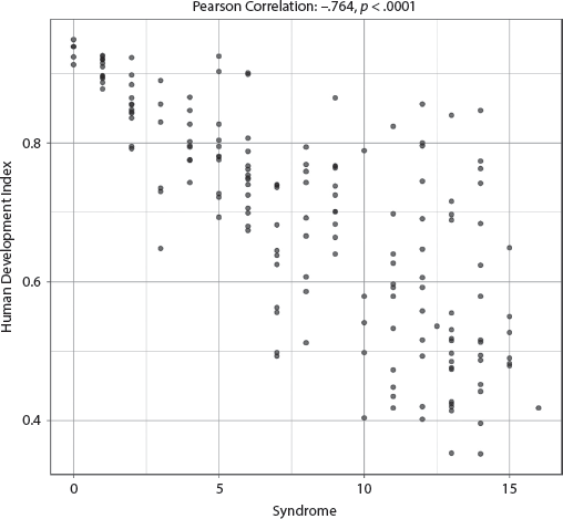
FIGURE 7.8.1 Scatterplot of Syndrome with Human Development Index

Because the Syndrome is significant in the general linear regression model, we also ran a logistic regression model (using a binary version of the response variable). The Syndrome and Urbanization are the only variables that are significant in predicting the logits or predicted probabilities of worse scores on the HDI. We specifically find that for every one unit increase in the Syndrome, the odds increase by 66 percent, or alternatively, the risk is 1.66 times greater that the country experiences lower scores on the HDI, after holding all other control variables constant.

8.2 Gender Inequality Index

(Higher scores are considered worse.)

The adjusted R-squared is a remarkably strong .718, indicating that the specified model explained at least 71.8 percent of the variability of the GII scores. Three variables reach significance: Syndrome with an effect size of .392, Urbanization with an effect size of .123, and Ethnic Fractionalization with an effect size of .078. We note that the effect size of the Syndrome is three and a half times larger than that of Urbanization. See appendix III, table AIII.7.8.2, for full results. The coefficient of Syndrome is positive, which means that Syndrome countries are more likely to rank high on the GII. The Urbanization coefficient is negative, which means that more urbanized countries are less likely to rank high on the GII. There is a very strong correlation between Syndrome and GII (r = .800, p < .0001). The scatterplot in figure 7.8.2 shows a strong upward pattern that substantiates the correlation between the two factors. The strong relationship between Syndrome and this index mirrors the strong correlation between Syndrome and the HDI (see figure 7.8.1).

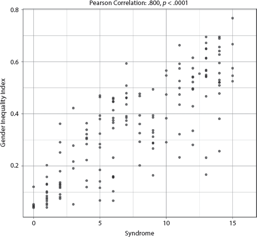
FIGURE 7.8.2 Scatterplot of Syndrome with Gender Inequality Index

Because the Syndrome is significant in the general linear regression model, we also ran a logistic regression model (using a binary version of the response variable). The Syndrome and Muslim Civilization are the only variables that are significant in predicting the logits or predicted probabilities of worse scores on the GII. We specifically find that for every one unit increase in the Syndrome, the odds increase by 81 percent, or alternatively, the risk is 1.81 times greater that the country scores worse on the GII, after holding all other control variables constant.

8.3 Happiness Index

(Lower scores are considered worse.)

The adjusted R-squared is a strong .643, indicating that the specified model explained at least 64.3 percent of the variability of the Happiness Index scores. Three variables prove significant: Muslim Civilization (effect size .080), the Syndrome (.242), and Urbanization (.222). See appendix III, table AIII.7.8.3, for full results. The effect size of Syndrome is a little larger than Urbanization, and both are around three times the effect size of Muslim Civilization. The coefficients for Muslim Civilization and Urbanization are positive, which means that these countries rank higher on the Happiness Index. The Syndrome’s coefficient is negative, which means that countries high on Syndrome rank significantly lower on the Happiness Index.

The bivariate correlation is significant and moderately strong at −.662 (p < .0001). The scatterplot in figure 7.8.3 illustrates this relationship with a strong negative pattern showing that countries higher on Syndrome have citizens who are less happy. We note that in the lower-right quadrant, we find both Muslim and non-Muslim countries: Syria and Afghanistan are majority Muslim countries, but Togo, Burundi, and Benin are not majority Muslim.

FIGURE 7.8.3 Scatterplot of Syndrome with Happiness Index

Because the Syndrome is significant in the general linear regression model, we also ran a logistic regression model (using a binary version of the response variable). The Syndrome and Urbanization are the only variables that are significant in predicting the logits or predicted probabilities of worse scores on the Happiness Index. We specifically find that for every one unit increase in the Syndrome, the odds increase by 45 percent, or alternatively, the risk is 1.45 times greater that the country scores worse on the Happiness Index, after holding all other control variables constant. That is noteworthy: all, and not just women, are significantly less happy when the first sexual political order is based on subordination, coercion, and exploitation of women—including men.

We use the World Health Organization’s female suicide rates as an ancillary variable and the GLM analysis yields a very low adjusted R-squared value of .097 with no significant independent variables. In our experience, we have found that the existing data on female suicide rates are patently not reliable, and so this is not an unexpected finding. In the future, we hope to create a scale to overcome some of the data deficiencies for female suicide, as this is an important relationship to examine.

8.4 Percentage of Pensionable-Age Persons Receiving Social Security or Pensions

(Lower scores are considered worse.)

The adjusted R-squared is a strong .533, indicating that the specified model explained at least 53.3 percent of the variability of the percentage of pensionable aged persons receiving social security or pensions. One variable, Syndrome, achieves significance with an effect size of .330. See appendix III, table AIII.7.8.4, for full results. Its coefficient is negative, which means that Syndrome countries are far less likely to provide retirement-age individuals with social security or pensions, which corroborates our hypotheses. The bivariate correlation is a very strong at −.718 (p < .0001). The scatterplot in figure 7.8.4 shows a downward slope. The distribution is complicated by a number of outliers for mid- and high-Syndrome scores. A number of Syndrome countries (e.g., Central Asia) were part of the former Union of Soviet Socialist Republics. These countries have a history of strong government involvement in care for elderly. Most other high-Syndrome countries expect kinship units to care for their elderly. Sons, in particular, are traditionally assigned the duty of caring for their parents in need or old age. As we have seen in previous chapters, the expectation that sons care for their parents is also a factor in son preference as well as in higher birth rates as families desire sons to guarantee their security in their old age. In the upper-left quadrant, we have Norway, Iceland, New Zealand, and Australia, which all are low on the Syndrome and high on those of retirement-age people receiving social security or pensions. In the upper-right quadrant, we have Lesotho, which is high on Syndrome and high on those of retirement age receiving social security or pensions. In the lower-right quadrant, we find Afghanistan, Yemen, Lebanon, and Chad, which are high on the Syndrome and low on those of retirement-age people receiving social security or pensions.

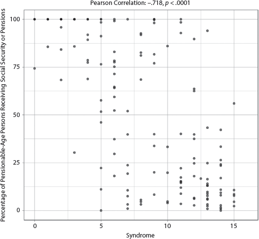
FIGURE 7.8.4 Scatterplot of Syndrome with Percentage of Pensionable-Age Persons Receiving Social Security or Pensions

Because the Syndrome is significant in the general linear regression model, we also ran a logistic regression model (using a binary version of the response variable). The Syndrome is the only variable that is significant in predicting the logits or predicted probabilities of lower percentages of pensionable-age people receiving social security or pensions. We specifically find that for every one unit increase in the Syndrome, the odds increase by 86 percent, or alternatively, the risk is 1.86 times greater that the country experiences lower percentages of pensionable-age persons receiving social security or pensions, after holding all other control variables constant. This corroborates our proposition that nations without pension schemes are, in effect, prodding their citizens to rely on the Patrilineal/Fraternal Syndrome. It may also be the case that when the Syndrome is strong, nations see no need to provide pensions. Given the totality of our findings, that is a short-sighted conclusion.

We use Social Safety Nets as an ancillary variable and the GLM analysis results in a high adjusted R-squared value of .509, for which the Syndrome is a significant predictor of this outcome variable, along with Urbanization, both in the expected direction.

8.5 Percent of Population with Access to Electricity

(Lower scores are considered worse.)

The adjusted R-squared is a strong .495, indicating that the specified model explained at least 49.5 percent of the variability of access to electricity. Three indicators are significant: Muslim Civilization (effect size .088), Syndrome (.099), and Urbanization (.152). See appendix III, table AIII.7.8.5, for full results. The coefficients for Muslim Civilization and Urbanization are positive, which means that majority Muslim countries and countries that are more urbanized have greater access to electricity on a per capita basis. The populations of Syndrome countries have less access to electricity on a per capita basis. The bivariate correlation is a moderately strong −.569 (p < .0001). As the scatterplot in figure 7.8.5 shows, the relationship between electricity per capita and the Syndrome is uneven. Although some Syndrome countries have excellent access to electricity, a number of countries have less access. Some countries rank medium on Syndrome, but have little access to electricity. Not unexpectedly, countries in the upper-left quadrant, which are low on the Syndrome but high on access to electricity, include Switzerland, the United States, and Spain. In the upper-right quadrant, countries that are high on the Syndrome and also high on access to electricity, include Iraq, Pakistan, Saudi Arabia, and Iran. Countries in the lower-right quadrant, which are high on the Syndrome and low on access to electricity, include South Sudan, Chad, Central African Republic, and Liberia.

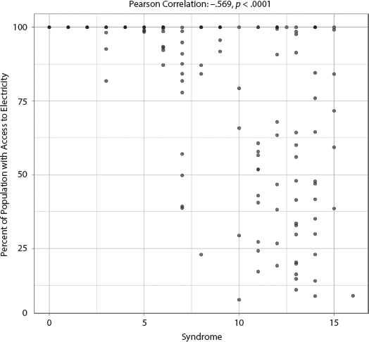
FIGURE 7.8.5 Scatterplot of Syndrome with Percent of Population with Access to Electricity

Because the Syndrome is significant in the general linear regression model, we also ran a logistic regression model (using a binary version of the response variable). The Syndrome, Urbanization, and Muslim Civilization are the only variables that are significant in predicting the logits or predicted probabilities of lower percentages of the population with access to electricity (less than 93.3 percent). We specifically find that for every one unit increase in the Syndrome, the odds increase by 35 percent, or alternatively, the risk is 1.35 times greater that the country experiences lower access to electricity, after holding all other control variables constant.

8.6 Hofstede Individualism Score

(Higher scores are associated with more individualistic cultures.)

The adjusted R-squared is a strong .471, indicating that the specified model explained at least 47.1 percent of the variability of the Hofstede Individualism Scores. The only significant predictor variable was the Syndrome, with a negative coefficient, which means the higher the Syndrome score, the less individualistic the culture. See appendix III, table AIII.7.8.6, for full results. This certainly makes sense in that the Syndrome imposes, shall we say, a lack of individualism particularly on all women, and the clan network also embeds men less as individuals and more as lineage representatives. The correlation with the Syndrome is a moderately strong −.621 (p < .0001), and the scatterplot in figure 7.8.6 shows the bivariate relationship between the Syndrome and individualism.

FIGURE 7.8.6 Scatterplot of Syndrome with Hofstede Individualism Score

Because the Syndrome is significant in the general linear regression model, we also ran a logistic regression model (using a binary version of the response variable). The Syndrome is the only variable that is significant in predicting the logits or predicted probabilities of a country experiencing worse Hofstede Individualism Scores. We specifically find that for every one unit increase in the Syndrome, the odds increase by 35 percent, or alternatively, the risk is 1.35 times greater that the country scores lower on the Hofstede Individualism measure, after holding all other control variables constant.

8.7 Gender Gap Index

(Lower scores are considered worse.)

The adjusted R-squared is a strong .445, indicating that the specified model explained at least 44.5 percent of the variability of GGI scores. The only variable that is significant in this model is the Syndrome, with an effect size of .318. See appendix III, table AIII.7.8.7, for full results. The variable’s coefficient is negative, which means that Syndrome countries rank worse on the GGI, which, in turn, means that Syndrome countries have larger gaps between men’s and women’s achievement as measured on subindices of Health and Survival, Educational Attainment, Economic Participation and Opportunity, and Political Empowerment. The bivariate correlation is a moderately strong −.670 (p < .0001). The scatterplot in figure 7.8.7 shows that high-Syndrome countries are slightly more likely to have more significant gender gaps. We identify some of the outliers in the plot. The country with the lowest (worst) score on the GGI is Yemen, with a Syndrome score of 15. Additionally, the three countries with the highest (best) scores on the GGI include Iceland, Finland, and Norway.

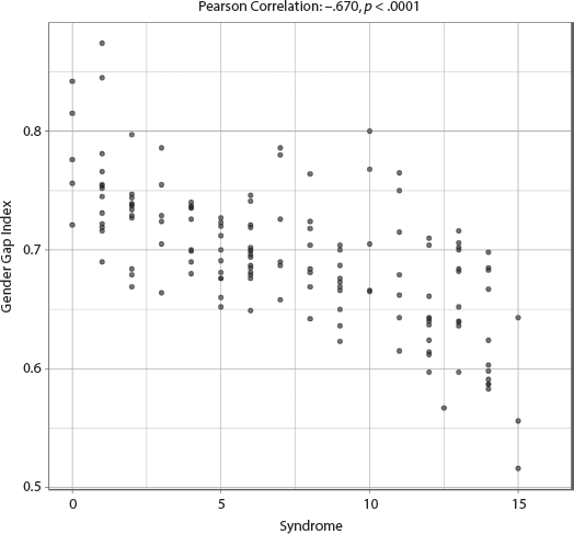
FIGURE 7.8.7 Scatterplot of Syndrome with Gender Gap Index

Because the Syndrome is significant in the general linear regression model, we also ran a logistic regression model (using a binary version of the response variable). The Syndrome is the only variable that is significant in predicting the logits or predicted probabilities of worse scores on the GGI. We specifically find that for every one unit increase in the Syndrome, the odds increase by 55 percent, or alternatively, the risk is 1.55 times greater that the country will score worse on the GGI, after holding all other control variables constant.

8.8 Discrimination and Violence Against Minorities

(Higher scores are considered worse.)

The adjusted R-squared is a moderate .399, indicating that the specified model explained at least 39.9 percent of the variability of discrimination and violence against minorities. Two variables prove significant: Syndrome and Number of Land Neighbors. The effect sizes are .097 and .141, respectively. See appendix III, table AIII.7.8.8, for full results. The coefficients for both are positive, which means that discrimination and violence against minorities increases the higher on the Syndrome scale a country ranks and the more land neighbors a country has. Thus, given more potentially competitive or even hostile neighbors on a state’s border, a state tends to discriminate, often violently, against outsiders in country. The bivariate correlation is a moderately strong .545 (p < .0001). The scatterplot in figure 7.8.8 bears out the bivariate relationship between the Syndrome and discrimination and violence against minorities in a positive trend. The three low-Syndrome and low–Discrimination and Violence Against Minorities countries in the lower-left quadrant are Sweden, Finland, and Iceland. These data support our claim that high-Syndrome countries are associated with harsher attitudes and policies toward citizens outside the majority national groups.

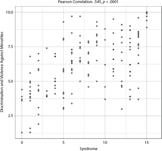
FIGURE 7.8.8 Scatterplot of Syndrome with Discrimination and Violence Against Minorities

Because the Syndrome is significant in the general linear regression model, we also ran a logistic regression model (using a binary version of the response variable). Although the model does meet the validity requirements, the Syndrome is not significant in this model (p = .03), and we do not report the results.

We use two variables in ancillary analyses to supplement the Discrimination and Violence Against Minorities analysis. We find a comparable adjusted R-squared value of .324 for Religious Tolerance, with Number of Land Neighbors, the Syndrome and Colonial Heritage Status as significant independent variables with the expected directionality (e.g., the higher/worse the Syndrome, the lower the level of religious tolerance). The second ancillary variable used, Tolerance for Immigrants, had a low adjusted R-squared value of .089 and the GLM analyses showed no significant predictors. Given that two of the variables in this cluster support our hypothesis, we are unclear why the third would not; there may be issues of operationalization at work in this last result. For this reason, we attempt to run multiple related indices, given the vagaries of operationalization, so that we may triangulate the results.

8.9 Legal Declaration of Gender Equality

(Higher scores are considered worse.)

The adjusted R-squared is a moderate .384, indicating that the specified model explained at least 38.4 percent of the variability of this scale on Legal Declaration of Gender Equality. One variable, the Syndrome, achieves significance with an effect size of .270. See appendix III, table AIII.7.8.9, for full results. The coefficient is positive, which means that Syndrome countries are more likely to sign on to the United Nations Legal Declaration of Gender Equality. This variable looks at the extent to which states codify gender equality in law, whether in its constitution or through legislation. This declaration is scaled in three levels, with higher scores showing less legal commitment to gender equality. Level 2 reflects no meaningful legal declaration for the country. Level 1 countries have nondiscrimination legislation only or customary law prioritized. Level 0 countries have enacted constitutional or comprehensive legal frameworks for gender equality. The scatterplot in figure 7.8.9 shows how countries are distributed along these three levels, and the relationship is significant (ANOVA F = 67.41, p < .0001). Generally speaking, high-Syndrome countries have no or little constitutional language or legislation committed to gender equality. Level 2 also denotes the countries where customary or personal laws are valid sources of law even if they violate legal provisions of nondiscrimination or equality. It is important to note that high-Syndrome countries scoring at level 0 or 1 on this outcome measure are not likely to fully implement their legal and constitutional commitments to gender equality, even if they have made such commitments. For example, countries in the lower-left quadrant, which are low on the Syndrome and have legal guarantees for gender equality, include Switzerland and the United Kingdom. In the lower-right quadrant, the countries include Somalia and the Solomon Islands, which are high on the Syndrome and also have legal guarantees for gender equality. Because of their Syndrome scores, we are more suspicious that Somalia and the Solomon Islands may not be implementing these guarantees than we are of Switzerland and the United Kingdom.

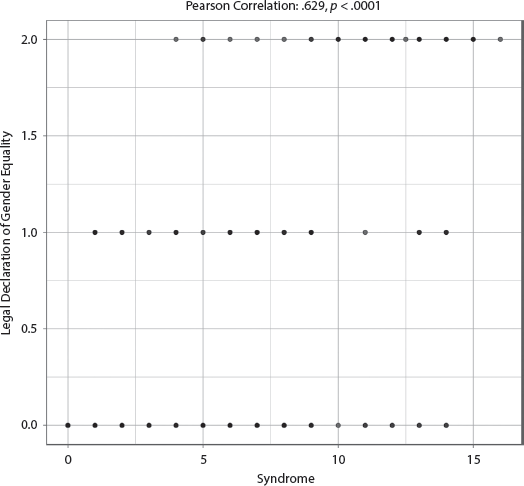
FIGURE 7.8.9 Scatterplot of Syndrome with Legal Declaration of Gender Equality

Because the Syndrome is significant in the general linear regression model, we also ran a logistic regression model (using a binary version of the response variable). The Syndrome is the only variable that is significant in predicting the logits or predicted probabilities of no gender equality or nondiscrimination clause in the constitution or legislation. We specifically find that for every one unit increase in the Syndrome, the odds increase by 69 percent, or alternatively, the risk is 1.69 times greater that the country does not have a gender equality or nondiscrimination clause in either its constitution or any legislation, after holding all other control variables constant.

We use three variables in ancillary analyses. The GLM analysis for Government Framework for Gender Equality has an adjusted R-squared value of .254, with the Syndrome as the only significant independent variable, and with the expected directionality. This finding is consistent with the results of the main analysis. The Formal Commitment to CEDAW variable has an adjusted R-squared value of .125, and the Syndrome is not a significant independent variable in the GLM analysis. Similar results are obtained for Presence of National Gender Equality Action Plan, which has a much lower adjusted R-squared value of .044. These are noteworthy negative results, indicating that ratifying CEDAW and having a national gender equality action plan may not necessarily correlate with the actual empowerment of women, but that having a formal declaration of the legal equality of women, or a government framework for gender equality, may indicate greater state commitment. Even so, the adjusted R-squared values are moderate for these variables.

Concluding Discussion for the Social Progress Dimension

Of the sixteen dependent variables measuring Social Progress examined here, the Syndrome proved significant for twelve. For five of the twelve dependent variables or factors for which the Syndrome was significant in multivariate modeling, it was the only variable demonstrating significance, and in another two models, it was the variable with the largest effect size. Other control variables that helped the explanatory power of the models included Urbanization, Ethnic Fractionalization, Civilization, and Number of Land Neighbors. Yet the Syndrome is far more consistent in its explanatory effects than these other variables.

Each of these social progress outcomes provides valuable information for our argument. Two areas prove particularly important. Development experts constructed the HDI to provide a more comprehensive measure of state development. By measuring life expectancy, educational attainment, and gross national income, the concept of development becomes multidimensional and provides a more accurate depiction of the condition of a state than is possible by measuring only GDP. The bivariate correlation between the Syndrome and HDI is extremely strong, and thus the Syndrome becomes an excellent predictor of negative outcomes regarding human development. We note that our empirical analysis includes data on the Syndrome’s relation to each of the three major areas measured by HDI and refer readers to our other dimensions for results on the Syndrome’s relation to health and life expectancy, educational attainment, and economic performance. Also noteworthy was the strong association between high Syndrome score and generalized societal levels of unhappiness. The subordination of women does not lead to a happy society for anyone, even men.

The second area that deserves attention is the poor correlation between variables that concern gender: Formal Commitment to CEDAW showed no correlation to Syndrome, Presence of National Gender Equality Action Plan showed no correlation to Syndrome, Legal Declaration of Gender Equality showed a significant but low correlation to Syndrome, Government Framework for Gender Equality showed a moderately low correlation to Syndrome, GGI showed a moderately low correlation to Syndrome, and GII showed a moderately high correlation to Syndrome.

One would expect that Syndrome as a negative measure of women’s well-being would correlate significantly with all of these six variables. The results, however, are diverse. The lack of correlation between Syndrome and Formal Commitment to CEDAW and Presence of National Gender Equality Action Plan suggests that states may sign on to international accords like CEDAW, or adopt international standards such as the National Gender Equality Plan without following through on reforms that would improve women’s well-being at the household level. In the case of CEDAW, states may either ignore the international standards, not have resources to commit to policy changes, or join only for face value. The relatively low correlation between Legal Declaration of Gender Equality and Government Frameworks for Gender Equality may reflect more rhetoric than real state effort and achievement.

The GGI and the GII show respectable correlations with our multivariate model, and in the case of the latter, a strong correlation. We already knew the bivariate associations from chapter 3, for which we used these variables to help validate the Syndrome index, but we wanted to see a fuller picture through multivariate analysis. We suggest that those two indexes capture effects of the Syndrome in their index compositions. Many of the commonly used variables to indicate women’s well-being are, in our judgment, secondary factors that are visible and easily measured, such as education rates, health and life expectancy, labor force participation, and women’s participation in government. Our theoretical framework holds that the Syndrome focuses on the practices embedded in informal social organizations that subsequently give rise to these more visible indicators of women’s status.

Another item of interest is the robust relationship between subordinating women and not providing pensions. The subordination of women, in a sense, substitutes for pension provision through the Syndrome’s components, including patrilocal marriage and lesser property and inheritance rights for women.

Last, the subordination of women is associated with significantly higher rates of discrimination against and violence toward minorities, which corroborates not only our theoretical framework but also the findings of scholars such as Elin Bjarnegard and Erik Melander. Hating “the other” has its roots in the character of male-female relations within the society.

Dimension 9. Environmental Protection

We hypothesize that countries with worse Syndrome scores will experience lower air quality, lower levels of environmental protection, and higher risks from environmental factors. We predict that societies that subordinate and exploit women also subordinate and exploit Mother Earth.

Analyses for the Environmental Protection Dimension

We perform four main analyses in the Environmental Protection dimension. The first looks at the Water and Environmental Well-Being factor, on which four indicators loaded in factor analysis. These four variables include Water and Sanitation, a subcomponent of the Environment Performance Index, which evaluates quality of sanitation and drinking water; the Environmental Performance Index itself, which is a respected measure giving an overall sense of a country’s performance on environmental issues, which includes health impacts, air quality, water and sanitation, water resources, agriculture, biodiversity and climate, and energy; Wastewater Treatment gauges the percentage of produced wastewater treated by centralized treatment facilities; and Foundations of Well-Being combines indicators of the country’s access to basic knowledge, access to information and communications, health and wellness, and environmental quality. We then conduct two ancillary analyses using the Environmental Performance Index separately and also Air Quality, which measures air quality by assessing household fuel use and minute atmospheric particulate matter (PM2.5).

The second analysis uses the Air Pollution Factor as the main analysis. Two indicators loaded on this factor: Household Indoor Air Pollution Attributable Deaths, which measures deaths that can be attributed to illnesses linked to household air pollution, and Greenhouse Gases, which measures emissions of carbon dioxide, methane, nitrous oxide, hydrofluorocarbons, perfluorocarbons, and sulfur hexafluoride. The ancillary analysis performed used Outdoor Air Pollution Attributable Deaths, which measures the rate of deaths resulting from emissions from households, industry, and vehicles per one hundred thousand people.

The third analysis is the Biodiversity and Pest regulation factor. Two indicators load on this factor, including Biodiversity and Habitat, which measures the percentage of naturally occurring community of flora and fauna in protected areas against the communities naturally occurring nationally, and Pesticide Regulation, a subcomponent of the Environmental Performance Index, which measures whether countries allow, restrict, or ban twelve toxic chemical pollutants used in agriculture, industry, and household products.

The fourth analysis has one variable, the Global Climate Risk Index, which assesses the impact of weather-related events (e.g., floods, hurricanes, heat waves) on nation-states.

Model Results

We ran seven general linear model analyses under Environmental Protection and found that the Syndrome was significant in six of those seven models. The model for which the Syndrome is not significant is the one that involves the Global Climate Risk Index. Table 7.9 summarizes the results of the GLM analyses

TABLE 7.9 Summary of GLM Results for the Environmental Protection Dimension in Descending Order of R-squared Values

Dependent Variables	Adjusted R-squared (N)	Independent Variables (significant at .001 by descending order of effect size)
1. Water and Environmental Well-Being Factor •   Water and Sanitation •   Environmental Performance Index •   Wastewater Treatment •   Foundations of Well-Being	.808 (149)	Urbanization Syndrome Ethnic Fractionalization Colonial Heritage Status
Environmental Performance Index	.639 (171)	Syndrome Urbanization
Air Quality	.411 (172)	Syndrome Terrain Urbanization
2. Air Pollution Factor •   Household Indoor Air Pollution Attributable Deaths •   Greenhouse Gases Emissions	.587 (156)	Urbanization Syndrome
Outdoor Air Pollution Attributable Deaths	.383 (160)	Syndrome Number of Land Neighbors
3. Biodiversity and Pest Regulation Factor •   Biodiversity •   Pest Regulations	.207 (160)	Syndrome
4. Global Climate Risk Index	.022 (172)	None

Note: Ancillary analyses in italics.

9.1 Water and Environmental Well-Being Factor

(This factor combines several variables: Water and Sanitation, Environmental Performance Index, Wastewater Treatment, and Foundations of Well-Being. Lower scores are considered worse.)

The adjusted R-squared is a remarkably strong .808, indicating that the specified model impressively explained at least 80.8 percent of the variability of this factor. We find that Colonial Heritage Status, Patrilineal/Fraternal Syndrome, Urbanization, and Ethnic Fractionalization are all significant variables in this model. See appendix III, table AIII.7.9.1, for full results. We note that Syndrome does not have the largest effect size for this model, but that the effect size of Urbanization is only slightly larger than Syndrome, and that Syndrome’s effect size is more than three times as large as the other two significant variables.

We would expect that a country’s level of urbanization would be the best predictor of water and environmental well-being, but we are surprised to find that the Syndrome is significant even when controlling for Urbanization and that its effect size is only slightly smaller than that variable. This is a noteworthy result to find that while we might expect only urbanization to affect water and environmental well-being, the Syndrome has a significant and almost as large of an impact. The sign of the Syndrome coefficient is in the predicted direction (negative, meaning the higher/worse the Syndrome score, the worse the water and environmental well-being).

We additionally find that countries that have never been colonized have better water and environmental well-being scores. We also find that countries with higher levels of Ethnic Fractionalization have lower levels of water and environmental well-being, suggesting that the more a country is fractionalized, the less it will focus on treating and sanitizing its water and their environmental well-being, on average.

In further analysis, we note the correlation between the Syndrome and the Water and Environmental Well-Being is a very strong −.783 (p < .0001), as shown in the scatterplot in figure 7.9.1. The lowest scores for Water and Environmental Well-Being are found only for countries with worse Syndrome scores. Additionally, although some outliers with higher scores appear in the upper-right quadrant, we find that only countries with the best Syndrome scores achieve the highest levels of Water and Environmental Well-Being. The six outliers in the upper-right quadrant include the United Arab Emirates, Qatar, Bahrain, Kuwait, Lebanon, and Saudi Arabia. The outlier in the lower-left quadrant is Mongolia, with a Syndrome score of 3 and a Water and Environmental Well-Being score of −2.2.

FIGURE 7.9.1 Scatterplot of Syndrome with Water and Environmental Well-Being Factor

Because the Syndrome is significant in the general linear regression model, we also ran a logistic regression model (using a binary version of the response variable). The Syndrome and Urbanization are the only variables that are significant in predicting the logits or predicted probabilities of worse water and environmental well-being. We specifically find that for every one unit increase in the Syndrome, the odds increase by 55 percent, or alternatively, the risk is 1.55 times greater that the country experiences worse water and environmental well-being, after holding all other control variables constant.

We performed two ancillary analyses using the Environmental Performance Index by itself and also Air Quality. The GLM analyses yield high adjusted R-squared values of .639 and .411, respectively, and the Syndrome is a significant predictor of both outcome variables.

9.2 Air Pollution Factor (Without Outlier)

(This factor combines two variables: Household Indoor Air Pollution Attributable Deaths and Greenhouse Gases; higher scores are considered worse.) We identified an extreme outlier in the data, the Central African Republic (score of 13.07), and thus we present the model with that one outlier removed.

The adjusted R-squared is a strong .587, indicating that the specified model explained at least 58.7 percent of the variability of this factor without the outlier, which was much higher than the adjusted R-squared with the outlier. We find that Patrilineal/Fraternal Syndrome and Urbanization are both significant in this model. See appendix III, table AIII.7.9.2, for full results. We note that the Syndrome has a smaller effect size compared with Urbanization in this model. We are again impressed that the Syndrome is significantly associated with air quality even when controlling for a country’s level of urbanization. We find that the sign of the Syndrome coefficient is in the predicted direction (positive, meaning the worse the Syndrome score, the worse the air pollution).

We further note that the direction of the coefficient for Urbanization is negative, which indicates that as the level of urbanization increases, a country’s air pollution decreases on average. This finding is counterintuitive, but it may indicate diminished use of wood-burning stoves in more urbanized environments.

In further analysis, we note the correlation between the Syndrome and the Air Pollution Factor (when the outlier is removed) is a moderately strong .604 (p < .0001) as shown in the scatterplot in figure 7.9.2. The slope in the scatterplot is not very steep, but we do find that only countries with the worst Syndrome scores have the highest (worst) values for the Air Pollution Factor.

FIGURE 7.9.2 Scatterplot of Syndrome with Air Pollution Factor

Because the Syndrome is significant in the general linear regression model, we also ran a logistic regression model (using a binary version of the response variable). The Syndrome and Urbanization are the only variables that are significant in predicting the logits or predicted probabilities of higher levels of air pollution. We specifically find that for every one unit increase in the Syndrome, the odds increase by 39 percent, or alternatively, the risk is 1.39 times greater that the country experiences higher levels of air pollution, after holding all other control variables constant.

We use Outdoor Air Pollution Attributable Deaths as an ancillary variable and the analysis yields an adjusted R-squared value of .383. The Syndrome is also a significant predictor for this outcome variable.

9.3 Biodiversity and Pest Regulation Factor

(This factor combines two variables: Biodiversity and Pesticide Regulation. Lower scores are considered worse.)

The adjusted R-squared is a moderate .207, indicating that the specified model explained at least 20.7 percent of the variability of this factor. We find that Patrilineal/Fraternal Syndrome is the only significant variable in this model, and has the largest effect size. See appendix III, table AIII.7.9.3, for full results. The sign of the Syndrome coefficient is in the predicted direction (negative, meaning the worst the Syndrome score, the lower the pest regulation and biodiversity in a country), corroborating our hypothesis.

In further analysis, we note the moderately strong correlation between the Syndrome and the Biodiversity and Pest Regulation factor (r = −.482, p < .0001) as shown in the scatterplot in figure 7.9.3. We find that the worst scores for the factor are found only in countries with worse (higher) Syndrome scores. Additionally, we find that only countries with the best Syndrome scores achieve the highest levels of biodiversity and pest regulation. Because the Syndrome is significant in the general linear regression model, we also ran a logistic regression model (using a binary version of the response variable). Because the model does not meet the validity requirements, we do not report the results.

FIGURE 7.9.3 Scatterplot of Syndrome with Biodiversity and Pest Regulation Factor

9.4 Global Climate Risk Index

(Higher scores are considered worse.)

The GLM results for this variable yielded a very low adjusted R-squared value of .022 with no significant terms so we do not report the results. Climate risk may be due to factors whose origins lie outside of the nation-state’s control.

Concluding Discussion for the Environmental Protection Dimension

The Patrilineal/Fraternal Syndrome is a significant predictor variable in six of the seven analyses performed (this tally includes the subanalysis of the Air Pollution Factor without the one outlier). In four of those six analyses, the Syndrome is either the only significant determinant of the dependent variable or it has the largest effect size. In the other two models, we find that Urbanization has the strongest effect size, which is expected for environmental indicators. We find, however, that even in these two analyses, the Syndrome’s effect size is only slightly smaller than Urbanization. The outcome variables for which the Syndrome was the only significant predictor or had the largest effect size included the following:

•   Biodiversity and Pest Regulation factor

•   Outdoor Air Pollution Attributable Deaths

•   Air Quality

The outcome variables for which Syndrome was significant, and its effect size was only slightly smaller than Urbanization included the following:

•   Water and Environmental Well-Being Factor

•   Air Pollution Factor (Without Outlier)

These are noteworthy results. A wide variety of environmental indicators appear to be significantly determined by the degree to which the Patrilineal/Fraternal Syndrome is encoded within the behavior of the society. These results are especially interesting because Syndrome is still significant when Urbanization, which we might expect to better explain environmental factors, is controlled for. These results are consistent with our hypothesis—that is, that countries that care more for their women take better care of their environment. The concern for those who Manne calls “the givers”—women—appears to extend to another female-coded “giver,” Mother Earth.46

Overall Conclusion

These results raise several interesting points. First and foremost, the Syndrome matters, and it matters greatly—the Syndrome emerges as a consistent and useful predictor of national outcome measures. The Syndrome was significant in 87 out of the 122 general linear model analyses run (71.3 percent). More specifically, the Syndrome is significant for fifteen out of sixteen (93.8 percent) Political Stability and Governance analyses, fifteen out of twenty (75 percent) Security and Conflict analyses, ten out of sixteen (62.5 percent) Economic Performance analyses, one out of six (16.7 percent) Economic Rentierism analyses, seventeen out of twenty-four (70.8 percent) Health and Well-Being analyses, five out of seven (71.4 percent) Demographic Security analyses, six out of ten (60 percent) Education analyses, twelve out of sixteen (75 percent) Social Progress analyses, and six out of seven (85.7 percent) Environmental Protection analyses. Typically, in these models, the Syndrome also displayed the largest or second-largest effect size.

Furthermore, the odds ratios calculated from these analyses are well worth considering, and we present a summary table (table 7.10) of those analyses for which the Syndrome was significant in multivariate modeling and for which the model conditions for logistic regression were met.

TABLE 7.10 Syndrome Odds Ratio and Percentage for Performing Poorly from the Logistic Regression Results for Each Variable for Which the Syndrome Was Significant in the GLM Analysis

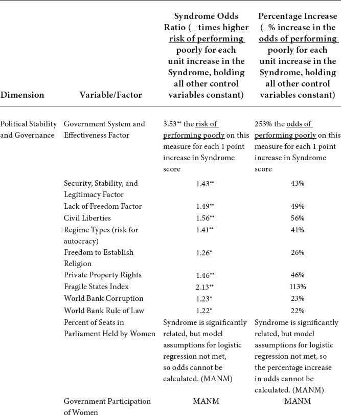
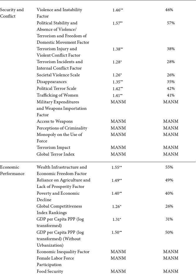
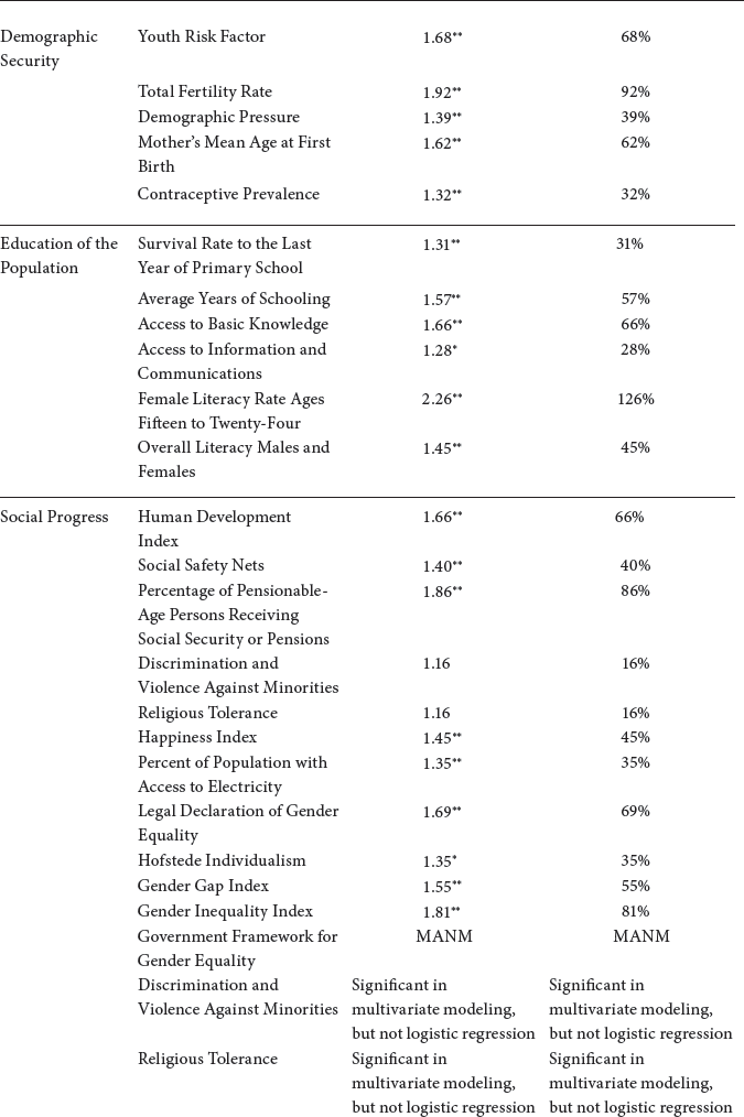
These numbers are illuminating. If a collective chooses a first, sexual political order based on the subordination of women to build up male-bonded kin networks as its preferred security provision mechanism, it will face a wide range of increasing probabilities of poor outcomes. For example, if women are subordinated through the Syndrome’s components, the collective will face 80 percent higher odds for hunger for every step up the Syndrome scale it goes, 66 percent increased odds for underweight children for every step, 41 percent increased odds for autocracy for every step, 50 percent increased odds for lower GDP for every step, 113 percent increased odds for state fragility for every step, 57 percent increased odds of political violence and terrorism for every step, 55 percent increased odds for poorer environmental quality for every step, 92 percent increased risk for high fertility for every step, 45 percent increased risk of national unhappiness for every step, and 253 percent increased odds of poor government effectiveness for every step. It is almost as if in choosing male-bonded kin networks as a security provision mechanism with its accompanying subordination of women, a collective chooses to curse itself.

The findings are so strong that we wonder why these multidimensional linkages between poor national outcomes and women’s subordination at the household level are not square one in both policy and scholarly conversations about national and international security. The Syndrome is the natural starting point for understanding outstanding differences in national stability, resilience, security, health, wealth, and well-being. As McDermott puts it, “If these findings were about something not related to women, chances are that they would be treated as revolutionary in international relations theory; indeed, the effects are much stronger than those supporting the notion of the democratic peace that has spawned an entire cottage industry of inquiry. I leave it to the reader to ponder why powerful effects regarding the treatment of women on the health and security of states do not receive such extensive attention.”47 That is a question well worth pondering, indeed.

Second, it is important to consider which control variables were significantly related to the outcome measures in addition to the Syndrome. Of the models for which the Syndrome was significant, Urbanization was the next most significant predictor followed by Ethnic Fractionalization, Number of Land Neighbors, and Muslim Civilization. The only variable that was never significant in these models was Hindu/Sinic/Buddhist Civilization, and Western Civilization was only significant in one model. As noted in part I, civilizational identity is not the engine of these poor results; it is the subordination of women at the household level that should draw our attention, instead. These findings tell us that Urbanization is clearly one important path to the amelioration of at least some components of the Syndrome, such as patrilocal marriage, whereas Ethnic Fractionalization and Number of Land Neighbors may represent societal stressors that synergize with and exacerbate the effects of Syndrome practices that subordinate women to their male-bonded kin/identity networks.

Third, it is also significant that the variability in outcome measures for high-Syndrome-scoring countries is much larger than for low-Syndrome-scoring countries. Sociologist Christine Bose has found a similar phenomenon, noting large variation for outcomes such as maternal mortality, adolescent fertility rates, female labor force participation, secondary education, and literacy ratios among societies that rank lower on measures of women’s empowerment.⁴⁸ The megaphone pattern of some of our scatterplots indicates that low-Syndrome countries have consistent “good” outcomes as measured by the security of the state and well-being of its citizens and environment. In contrast, high-Syndrome countries have a comparatively wide range of results, with most of these countries tending toward “bad” outcomes for the state, the people, and the environment.

Why this variation? Although a low Syndrome score appears to be “protective” of national outcomes, high-Syndrome countries operate without such protection. Even so, the potential for worse outcomes among high-Syndrome-encoding nations might be mitigated by a country’s wealth and natural resources. For example, a number of oil-rich countries in the Middle East have high Syndrome scores, but they also have some excellent outcomes in areas such as literacy and maternal mortality, and these excellent outcomes have been made possible by their remarkably high level of wealth. Should those extraordinary factors fade, however, we would expect a regression toward more typical (i.e., worse) high-Syndrome-score national outcomes. We identified the countries in our sample that had better-than-expected national outcomes given their relatively high Syndrome scores (see appendix V for details). These included Bahrain, Jordan, Kuwait, Malaysia, Oman, Qatar, Saudi Arabia, and the United Arab Emirates, but also, interestingly, Botswana. In future work, we would like to explore how a country like Botswana achieved such unusual national outcomes given its relatively high Syndrome score of 11. Social psychologist Khandis Blake suggests, for example, that Botswana has an unusually high rate of male labor migration and, as a result, there is less opportunity for patrilocality and many households are, perforce, female-headed households.⁴⁹ This deserves more in-depth investigation.

Our results show that when there is strong emphasis placed on the subordination of women at the household level via the Patrilineal/Fraternal Syndrome’s components due to reliance on male-bonded kin groups or clans for security, that societal choice is strongly associated with instability and insecurity, environmental degradation, low levels of well-being and prosperity for its citizens, poor governance and autocracy, and many other negative outcomes at the state level in aggregate statistical testing. Deepening that associational analysis, in previous chapters we have traced the causal mechanisms linking these variables, providing a clearer understanding of why these negative national outcomes obtain. But perhaps even more important, our results suggest that disruption of the Syndrome’s mechanisms might provide a path to greater stability and security for nations and the international system.

Is such change possible? Has it ever successfully happened before, and what have been the results? Have such attempts ever failed before, and if so, why did they fail? And what lessons for today might we derive? In part III, we turn to these important questions.