Chapter 1
Normed and Banach spaces
As we had discussed in the introduction, we wish to do calculus in vector spaces (such as C[a, b], whose elements are functions). In order to talk about the concepts from calculus such as differentiability, we need a notion of closeness between points of a vector space.
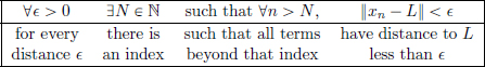
Recall for example, that a real sequence (an)n∈N is said to converge with limit L ∈ R if for every  > 0, there exists an N ∈ N such that whenever n > N, |an − L| < . In other words, the sequence converges to L if no matter what distance > 0 is given, one can guarantee that all the terms of the sequence beyond a certain index N are at a distance of at most away from L (this is the inequality |an − L| < ). So we notice that in this notion of “convergence of a sequence”, indeed the notion of distance played a crucial role. After all, we want to say that the terms of the sequence get “close” to the limit, and to measure closeness, we use the distance between points of R. A similar thing happens with continuity and differentiability. Recall that a function f : R → R is said to be continuous at c ∈ R if for every > 0, there exists a δ > 0 such that whenever |x − c| < δ, |f(x) − f(c)| < . Roughly, given any distance , I can find a distance δ such that whenever I choose an x not farther than a distance δ from c, I am guaranteed that f(x) is not farther than a distance of from f(c). Again notice the key role played by the distance in this definition. The distance between points x, y ∈ R is taken as |x − y|, where | · | : R → [0, ∞) is the absolute value function, given by
If we imagine the real numbers depicted on a “number line”, then |x − y| is the length of line segment joining x, y visualised on the number line. See the following picture.

But now if one wants to also do calculus in a vector space X (for example C[a, b]), there is so far no ready-made available notion of distance between vectors. One way of creating a distance in a vector space is to equip it with a “norm” || · ||, which is the analogue of absolute value | · | in the vector space R. The distance function is then created by taking the norm ||x − y|| of the difference between vectors x, y ∈ X, just like in R the Euclidean distance between x, y ∈ R was taken as |x − y|.
Having done this, we have the familiar setting of calculus, and we can talk about notions like the derivative of a function living on a normed space. (Later on, in Chapter 3, we will then also have analogues of the two facts from ordinary calculus relevant to optimisation, namely the vanishing of the derivative for minimisers, and the sufficiency of this condition for minimisation when the function is convex.) Thus the outline of this chapter is as follows.
First of all, we will learn the notion of a “normed space”, that is a vector space equipped with a “norm”, enabling one to measure distances between vectors in the vector space. This makes it possible to talk about concepts from calculus, and in particular the notion of differentiability of functions between normed spaces, as we shall see later on. Next, we will see lots of examples of normed spaces: we will see that1
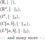
are all normed spaces, enabling us to do Calculus in each case.
Finally, we will introduce Banach spaces, which are special types of normed spaces, namely ones in which “Cauchy sequences converge”. We will also motivate this, and see why Banach spaces are nicer than having merely a normed space.
We begin by recalling the notion of vector space.
1.1Vector spaces
Roughly speaking it is a set of elements, called “vectors”. Any two vectors can be “added”, resulting in a new vector, and any vector can be multiplied by an element from R (or C, depending on whether we consider a real or complex vector space), so as to give a new vector. The precise definition is given below.
Definition 1.1. (Vector space) Let K = R or C (or more generally2 a field). A vector space over K, is a set X together with two functions, + : X × X → X, called vector addition, and · : K × X → X, called scalar multiplication that satisfy the following:
(V1)For all x1, x2, x3 ∈ X, x1 + (x2 + x3) = (x1 + x2) + x3.
(V2)There exists an element, denoted by 0 (called the zero vector) such that for all x ∈ X, x + 0 = x = 0 + x.
(V3)For every x ∈ X, there exists an element, denoted by −x, such that x + (−x) = (−x) + x = 0.
(V4)For all x1, x2 in X, x1 + x2 = x2 + x1.
(V5)For all x ∈ X, 1 · x = x.
(V6)For all x ∈ X and all α, β ∈ K, α · (β · x) = (αβ) · x.
(V7)For all x ∈ X and all α, β ∈ K, (α + β) · x = α · x + β · x.
(V8)For all x1, x2 ∈ X and all α ∈ K, α · (x1 + x2) = α · x1 + α · x2.
Example 1.1. (R). R is a vector space over R, with vector addition being the usual addition of real numbers, and scalar multiplication being the usual multiplication of real numbers. (R is also a vector space over the field Q of rational numbers, but we will always consider the real vector space R unless stated otherwise.)

Example 1.2. (Rd). Rd = R × · · · R (d times) is the set of all ordered d-tuples (x1, · · · , xd) of real numbers x1, · · · , xd . Then Rd is a vector space over R, with addition and scalar multiplication defined =component-wise”:
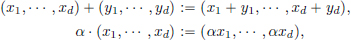
for (x1, · · · , xd), (y1, · · · , yd) ∈ Rd and α ∈ R.
Example 1.3. (C[a, b]). Let a, b ∈ R and a < b. Consider the vector space consisting of all continuous functions x : [a, b] → K, with addition and scalar multiplication defined in a “pointwise” manner as follows.
If x1, x2 ∈ C[a, b], then x1 + x2 ∈ C[a, b] is the function given by

If α ∈ K and x ∈ C[a, b], then α · x ∈ C[a, b] is the function given by

It can be checked that the vector space axioms (V1)-(V8) are satisfied. C[a, b] is referred to as a ‘function space’, since each vector in C[a, b] is a function (from [a, b] to K). The zero vector in C[a, b] is the zero function 0, given by 0(t) = 0 for all t ∈ [a, b].
Example 1.4. (C1[a, b]). Let C1[a, b] denote the space of continuously differentiable functions on [a, b]:

(Recall that a function x : [a, b] → R is continuously differentiable if for all t ∈ [a, b], the derivative of x at t, namely x′(t), exists, and the map t  x′(t) : [a, b] → R is a continuous function.) We note that
because whenever a function x : [a, b] → R is differentiable at a point t in [a, b], then x is continuous at t. In fact, C1[a, b] is a subspace of C[a, b] because it is closed under addition and scalar multiplication, and is nonempty:
(S1)For all x1, x2 ∈ C1[a, b], x1 + x2 ∈ C1[a, b].
(S2)For all α ∈ R, x ∈ C1[a, b], α · x ∈ C1[a, b].
(S3)0 ∈ C1[a, b].
Thus C1[a, b] is a vector space with the induced operations from C[a, b], namely the same pointwise operations as defined in (1.1) and (1.2).
Example 1.5. (Sequence spaces). For any real p such that 1  p < ∞,
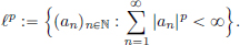
(Here we take the sequences (an)n∈N with values in K.) We define vector addition and scalar multiplication termwise:

for elements (an)n∈N, (bn)n∈N ∈ ℓp and α ∈ K. It is not yet clear whether the sum of two elements in ℓp, defined in the manner above, delivers an element in ℓp. That this is indeed true is shown by the elementary chain of inequalities below:

We can use these inequalities termwise, and the Comparison Test for convergence of real series, to conclude that (an)n∈N + (bn)n∈N ∈ ℓp whenever (an)n∈N, (bn)n∈N ∈ ℓp.
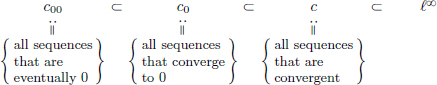
By ℓ∞ we denote the vector space of all bounded sequences with values in K, once again with termwise operations. It is easy to see that the sum of two elements from ℓ∞ is again an element of ℓ∞.
It is clear that ℓp ⊂ ℓ∞ for all p ∈ [1, ∞]: if (an)n∈N ∈ ℓp, then

and so  |an|p = 0. In particular, (an)n∈N is a bounded sequence.
So all the ℓp spaces with a finite p are subspaces of ℓ∞. Some other important subspaces are:
Example 1.6. (Lp[a, b]). For p ∈ [1, ∞], define
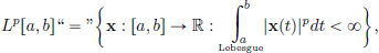
where the integral is the “Lebesgue integral” rather than the riemann integral.
What do we need to know about Lebesgue integrals? Firstly, every Riemann integrable function x on an interval [a, b] is also Lebesgue integrable on [a, b], and moreover, the Lebesgue integral then coincides with the usual Riemann integral. However, the class of Lebesgue integrable functions is much larger than the class of continuous functions. For instance, it can be shown that the function

is Lebesgue integrable, but not Riemann integrable on [0, 1]. For computation aspects, one can get away without having to go into technical details about Lebesgue integration. (In an appendix called “The Lebesgue Integral” on page 359, we have outlined the key definitions and a few relevant results on the Lebesgue Integral, which the reader might wish to read if so desired, in order to get a better feeling for the Lp spaces.)
We also note that in the above definition of Lp[a, b], we have put quotes around the equality sign. What is that supposed to mean? Strictly speaking, each element of Lp[a, b] is not a function x, but rather an equivalence class [x] of functions, where

(The reason for wanting Lp[a, b] to be this set of equivalence classes [x], rather than the functions x itself, will become clear when we discuss “norms”. It is tied to demanding that the only vector in Lp[a, b] with 0 norm must be the zero vector.) Of course, if x, y ∈ C[a, b], then
and thanks to the continuity of x, y, we could then conclude that

But it may happen for functions x, y ∈ Lp[a, b] that they are not equal as functions, but nevertheless

In fact if x is the function given by (1.3), and y = 0, then it turns out that

but clearly x ≠ y! Note however that in this example, “almost everywhere”, that is, for “almost all” t ∈ [0, 1], (only the rational t are excluded!) we do
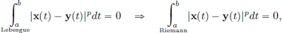
have x(t) = y(t). These phrases can be made precise using the theory of Lebesgue integral, in that it turns out that if

then x(t) = y(t) for all t ∈ [a, b]\N, where N has “Lebesgue measure” 0. We won’t go into this, but we’ll simply bear in mind that for

So we view elements of Lp[a, b] through “fuzzy glasses”, and treat two functions as being identical whenever the integral above is 0.
Analogous to the space ℓ∞, one can also introduce the space L∞[a, b]:

Since this example relies on the notion of Lebesgue measure, we won’t discuss this any further now.
Exercise 1.1. True or false? The set V = (0, ∞) (positive reals) is a vector space with addition and scalar multiplication given by x + y = xy and α · x = xα for all positive x, y, and for all α ∈ R.
Exercise 1.2. (C[0, 1] is not finite dimensional.) Show that C[0, 1] with the usual pointwise operations is not a finite dimensional vector space.
Hint: One can prove this by contradiction. Let C[0, 1] be a finite dimensional vector space with dimension d, say. First show that the set B = {t, t2, ···, td} is linearly independent. Then B is a basis for C[0, 1], and so the constant function 1 should be a linear combination of the functions from B. Derive a contradiction.
Exercise 1.3. Let S := {x ∈ C1[a, b] : x(a)= ya and x(b)= yb}, where ya, yb ∈ R. Prove that S is a subspace of C1[a, b] if and only if ya = yb = 0. (So we see that S is a vector space with pointwise operations if and only if ya = yb = 0.)
1.2Normed spaces
We would like to develop calculus in the setting of vector spaces (for example, in function spaces like C[a, b]). Underlying all the fundamental concepts in ordinary calculus, is the notion of closeness between points. So in order to generalise the notions from ordinary calculus (where we work with real numbers, and where the absolute value is used to measure distances), to the situation of vector spaces, we need a notion of distance between elements of the vector space. This is done by introducing an additional structure on a vector space, namely, a “norm”, which is a real-valued function || · || defined on the vector space, and the norm plays a role analogous to the one played by the absolute value in R. Once we have a norm on a vector space X (in other words a “normed space”), then the distance between x, y ∈ X will be taken as ||x − y||.
Definition 1.2. (Norm; normed space). Let X be a vector space over K (R or C). A norm on X is a function || · || : X → [0, +∞) such that:
(N1)(Positive definiteness).
For all x ∈ X, ||x||  0. If x ∈ X and ||x|| = 0, then x = 0.
(N2)For all α ∈ K (R or C) and for all x ∈ X, ||αx|| = |α|||x||.
(N3)(Triangle inequality) For all x, y ∈ X, ||x + y|| ||x|| + ||y||.
A normed space is a vector space X equipped with a norm.
Distance in a normed space. Just like in R, with the absolute value, and where the distance between x, y ∈ R is |x − y|, now in a normed space (X, || · ||), we have for x, y ∈ X, that the number ||x − y|| is taken as the distance between x, y ∈ X. Thus ||x|| = ||x − 0|| is the distance of x from the zero vector 0 in X.
Remark 1.1. (Metric spaces). A metric space is a set X together with a function d : X × X → R satisfying the following properties:
(D1)(Positive definiteness)
For all x, y ∈ X, d(x, y) 0. For all x ∈ X, d(x, x) = 0.
If x, y ∈ X are such that d(x, y) = 0, then x = y.
(D2)(Symmetry) For all x, y ∈ X, d(x, y) = d(y, x).
(D3)(Triangle inequality) For all x, y, z ∈ X, d(x, y) + d(y, z) d(x, z).
The reader familiar with “metric spaces” may notice that in a normed space (X, || · ||), if we define d : X × X → R by d(x, y) = ||x – y|| for x, y ∈ X, then it is easily seen that d satisfies (D1)-(D3), and so (X, d) is a metric space with the metric/distance function d. This distance d is referred to as the induced distance in the normed space (X, || · ||). Then ||x|| = ||x − 0|| = d(x, 0), and so the norm of a vector x in the normed space (X, || · ||) is the induced distance of x to the zero vector.
We now give a few examples of normed spaces, by reconsidering the vector space examples from the previous section, and equipping each of them with norms.
Example 1.7. (R, | · |). R is a vector space over R. Define || · || : R → R by ||x|| = |x|, for x ∈ R. Then (R, |·|) is a normed space. (No surprise, since wanting to generalise the situation from ordinary calculus in R to the case of vector spaces, | · | is what motivated the definition of the norm || · ||!)
Example 1.8. (Rd, || · ||p). Rd is a vector space over R. Let us define the Euclidean norm || · ||2 by

Then Rd is a normed space (see Exercise 1.8.(1) on page 16).
(The motivation behind calling (N3) the triangle inequality is now evident. Indeed, for triangles in Euclidean Geometry of the plane, we know that the sum of the lengths of two sides of a triangle is at least as much as the length of the third side. If we now imagine the points 0, –x, y ∈ R2 as the three vertices of a triangle, then this is what (N3) says for the || · ||2 norm; see the following picture.)

|| · ||2 is not the only norm3 that can be defined on Rd. For example,

are also examples4
Note that (Rd, || · ||2), (Rd, || · ||1) and (Rd, || · ||∞) are all different normed spaces. This illustrates the important fact that from a given vector space, we can obtain various normed spaces by choosing different norms. What norm is considered depends on the particular application at hand. We illustrate this in the next paragraph.
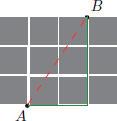
Imagine a city (like New York) in which there are streets and avenues with blocks in between, forming a square grid as shown in the picture below. Then if we take a taxi/cab to go from point A to point B in the city, it is clear that it isn’t the Euclidean norm in R2 which is relevant, but rather the || · ||1-norm in R2. (It is for this reason that the || · ||1-norm is sometimes called the taxicab norm.)
So what norm one uses depends on the situation at hand, and is something that the modeller decides. It is not something that falls out of the sky!
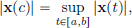
Example 1.9. (C[a, b] as a normed space). Consider the vector space C[a, b] defined earlier. Define

Then || · ||∞ is a norm on C[a, b], and is referred to as the “supremum norm.” The second equality above, guaranteeing that the supremum is attained, that is, that there is a c ∈ [a, b] such that
follows from the Extreme Value Theorem5 for continuous functions.
Exercise 1.4. In C[0, 1] equipped with the || · ||∞-norm, calculate the norms of t, –t, tn and sin(2πnt), where n ∈ N.
Let us check that || · ||∞ on C[a, b] does satisfy (N1), (N2), (N3).
(N1)For x ∈ C[a, b], |x(t)| 0 for all t ∈ [a, b]. So ||x||∞ =  |x(t)| 0.
Also, if x ∈ C[a, b] is such that ||x||∞ = 0, then for each t ∈ [a, b],
So for all t ∈ [a, b], |x(t)| = 0, and so x(t) = 0.
In other words, x = 0, the zero function in C[a, b].
(N2)If α ∈ R and x ∈ C[a, b], then |(α · x)(t)| = |αx(t)| = |α||x(t)|, for t ∈ [a, b], and so ||α · x||∞ =  |α||x(t)| = |α| |x(t)| = |α|||x||∞.
(N3)Let x1, x2 ∈ C[a, b]. If t[a, b], then

As this holds for all t ∈ [a, b], |(x1 + x2)(t)| ||x1||∞ + ||x2||∞.
Thus ||x1 + x2||∞ ||x1||∞ + ||x2||∞.
So C[a, b] with the supremum norm || · ||∞ is a normed space. Thus we can use ||x1 − x2||∞ as the distance between x1, x2 ∈ C[a, b].
Geometric meaning of the distance in C[a, b] equipped with the supremum norm. We ask the question: what does it mean geometrically when we say that x is close to x0? In other words, what does the set of points x that are close to (say within a distance of from) x0 look like?
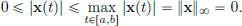
In (R, | · |), we know that the set of points x whose distance to x0 is less than is an interval:

and so {x ∈ R : |x − x0| < } = (x0 − , x0 + ).
Now we ask: can we visualise the set {x ∈ C[a, b] : ||x − x0||∞ < }? We have that

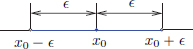
We can imagine translating the graph of x0 upward by a distance of , and downward through a distance of , so as to obtain the shaded strip depicted in the following picture. Then the graph of x has to lie in this shaded strip, because at each t, x0(t) − < x(t) < x0(t) + . So for example at the particular t indicated in the following picture, x(t) has to lie on the line segment AB. Since this has to happen at each t ∈ [a, b], we see that the graph of x lies in the shaded strip.

Fig. 1.1 The set of all continuous functions x whose graph lies between the two dashed curves is the “ball” B(x0, ) = ||x ∈ C[a, b] : {x − x0||∞ < }.
Here are examples of some other frequently used norms in C[a, b]:
for x ∈ C[a, b]. The || · ||1-norm can be thought of as a continuous analogue of the taxicab norm, while the || · ||2 norm is the continuous analogue of the Euclidean norm. The verification that || · ||1 is indeed a norm on C[a, b] will be done in Exercise 1.10. We’ll postpone checking that || · ||2 is also a norm on C[a, b] until Chapter 4, where we will first check that C[a, b] can be endowed with an “inner product”

and then
will automatically become a norm! right now we’ll just accept the fact that || · ||2 is a norm on C[a, b].
We will see later on that (C[a, b], || · ||∞) is “complete”, that is, {Cauchy sequences} = {convergent sequences}, while (C[a, b], || · ||2) is not complete. On the other hand, (C[a, b], || · ||2) has a “nicer geometry”, allowing one to talk about orthogonality6. What is the remedy? This motivates the consideration of (L2[a, b], || · ||2), which besides allowing the nice geometry, also turns out to be complete. We will introduce this normed space in Example 1.12 below.
Example 1.10. C1[a, b]. recall our optimal mining problem from Example 0.1, where the function to be minimised was defined on a subset of the subspace C1[a, b]. So we see that the space C1[a, b] also arises naturally in applications. What norm do we use in C1[a, b]? In general, if X is a normed space and Y is a subspace of the vector space X, then we can make Y into a normed space by simply using the restriction of the norm in X to Y. This is called the induced norm in Y, and in Exercise 1.7, we will see that this does give a norm on Y. So surely C1[a, b], being a subspace of C[a, b] (which is a normed space with the supremum norm), is also a normed space with the supremum norm || · ||∞. However, it turns out that in applications, this is not a good choice, essentially because the differentiation map

is not “continuous” (we will see this later on). There is a different norm on C1[a, b], denoted by || · ||1,∞, given below, which we shall use:

In C1[0, 1], for example
Roughly, two functions in (C1[a, b], || · ||1,∞) are regarded as close together if both the functions themselves and their first derivatives are close together. Indeed, ||x1 − x2||1,∞ < implies that

and conversely, (1.7) implies that ||x1 – x2||1,∞ < 2. We will see later (when discussing continuity of maps between normed spaces), that the differentiation mapping from C1[a, b] to C[a, b] is continuous if C1[a, b] is equipped with the || · ||1,∞-norm and C[a, b] is equipped with the || · ||∞-norm.
Example 1.11. (Sequence spaces). For 1 p < ∞, ℓp is a normed space with the || · ||p norm, given by

Checking that the triangle inequality holds can be done using an inequality called Hölder’s Inequality; see Exercise 1.8.
When p = ∞, that is, for the sequence space ℓ∞, we define
Then it is easy to check that || · ||∞ is a norm, and so (ℓ∞, || · ||∞) is a normed space.
Example 1.12. For 1 p < ∞, Lp[a, b] is the normed space with the || · ||p norm, given by

We won’t check the validity of (N3) here. Also, the space L∞[a, b] is a normed space with the norm given by

Again, we won’t try to make “almost all” precise, as it relies of the notion of Lebesgue measure. The || · ||∞-norm here is referred to as the “essential supremum norm”.
We remark that even more generally, if (Ω, M, μ) is any “measure space”, where μ is a positive measure, then Lp(Ω) denotes the collection of all real-valued measurable functions x on Ω with
It turns out that (Lp(Ω), || · ||p) is a normed space, which is moreover, complete. This normed space arises in applications, for example when (Ω, M, μ) is a probability space, where the x are “random variables”, and ||x||pp then has the interpretation of being the expected value E(|xp).
Exercise 1.5. (Triangle Inequality). Let (X, || · ||) be a normed space. Prove that for all x, y ∈ X, |||x|| – ||y|| – ||x − y}.
Exercise 1.6. If x ∈ R, then let ||x|| = |x| . Is || · || a norm on R?
Exercise 1.7. Let X be a normed space with norm || · ||X, and Y be a subspace of X. Prove that Y is also a normed space with the norm || · ||Y defined simply as the restriction of the norm || · ||X to Y. This norm on Y is called the induced norm.
Exercise 1.8. Let 1 < p < ∞ and q be defined by  .
.
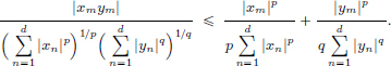
Then Hölder’s inequality says that if x1, ···, xd, y1, ···, yd ∈ C, then

Let’s quickly establish this inequality. Suppose that a, b ∈ R and a, b 0. We begin by showing that

If a = 0 or b = 0, then the conclusion is clear, and so we assume that both a and b are positive. We will use the following result.
Claim: If α ∈ (0, 1), then for all x ∈ [1, ∞), α(x − 1) + 1 xα.
Given α ∈ (0, 1), define fα : [1, ∞) → R by fα(x) = α(x − 1) – xα + 1, for x 1. Note that fα(1) = α · 0 − 1α + 1 = 0, and for all x 1,

By the Fundamental Theorem of Calculus, for any x > 1,

and so we obtain fα(x) 0 for all x ∈ [1, ∞), completing the proof of the claim. As p ∈ (1, ∞), it follows that 1/p ∈ (0, 1). Applying the above with α = 1/p and

we obtain inequality (1.8).
Holder’s inequality is obvious if  = 0 or
  = 0.
= 0.
So we assume that neither is 0, and proceed as follows.
Define am = |xm|p/ |xn|p and bm = |ym|q/ |yn|q, 1 m d.
Applying the inequality (1.8) to am, bm, we obtain for each m that:
Adding these d inequalities, we obtain Hölder’s inequality.
If 1 p ∞, and d ∈ N, then for x = (x1, ···, xd) ∈ Rd, define

(1)Show that the function x ||x||p is a norm on Rd.
Hint: In the case when 1 < p < ∞, use Hölder’s inequality to obtain

and use ||x + y||pp = |xn + yn||xn + yn|p–1
(2)Let d = 2. For 1 p ∞, the “open unit ball” Bp(0, 1), is defined by Bp(0, 1) := {x ∈ R2 : ||x||p < 1}. Sketch Bp(0, 1) for p = 1, 2, ∞.
(3)(Explanation of the notation for the maximum norm “|| · ||∞”.) Let x ∈ R. Prove that (||x||p)p∈N is a convergent sequence in R, and  ||x||p = ||x||∞. Describe qualitatively what happens to the sets Bp(0, 1) as p tends to ∞.
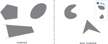
Exercise 1.9. A subset C of a vector space is said to be convex if for all x, y ∈ C, and all α ∈ (0, 1), (1 − α)x + αy ∈ C; see the following picture for examples of convex and nonconvex sets in R2.
(1)In any normed space (X, || · ||), show that the “closed unit ball”  defined by := {x ∈ X : ||x|| 1} is convex.
(2)Depict the set  in the plane.
(3)(Explanation of why we’ve been taking p in [1, ∞) rather than just all p > 0). Prove that  does not define a norm on R2.
Exercise 1.10. Show that (1.5) on page 12 defines a norm on C[a, b].
Exercise 1.11. Let Cn[a, b] be the set of n times continuously differentiable functions on [a, b]: Cn[a, b] = {x : [a, b] → R such that x′, x″, ···, x(n) ∈ C[a, b]}, equipped with pointwise operations, and the norm

Show that || · ||n,∞ is a norm on Cn[a, b].
Exercise 1.12. (“p-adic norm”). Consider the vector space of the rational numbers Q over the field Q. Let p be a prime number. If the integer q divides the integer n, we write q | n, and if not, then we write q  n.
n.
Define the p-adic norm  · p on Q as follows:
0p := 0, and if r ∈ Q\{0}, then rp :=  where
where 
So in this context, a rational number is close to 0 precisely when it is “highly divisible” by p.
(1)Show that · p is well-defined on Q.
(2)If r ∈ Q, then prove that rp 0, and that if rp = 0 then r = 0.
(3)For all r1, r2 ∈ Q, show that 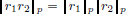 .
.
(4)For all r1, r2 ∈ Q, prove that  .
.
In particular, for all r1, r2 ∈ Q,  .
.
Exercise 1.13. Consider the vector space Rm×n of matrices with m rows and n columns of real numbers, with the usual entrywise addition and scalar multiplication. Let the entry in the ith row and jth column of M be denoted by mij. For M ∈ Rm×n, define  . Show that || · ||∞ is a norm on Rm×n.
1.3Topology of normed spaces
In a normed space, we can describe “neighbourhoods” of points by considering sets which include all points whose distance to the given point is not too large.
Definition 1.3. (Open ball).
Let (X, || · ||) be a normed space, x ∈ X, and r > 0.
The open ball B(x, r) with centre x and radius r is defined by

Thus B(x, r) is the set of all points in X whose distance to the centre x is strictly less than r.
We’ll keep the following picture in mind.
In the sequel, for example in our study of continuous functions, open sets will play an important role. Here is the definition.
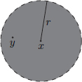
Definition 1.4. (Open set). Let (X, || · ||) be a normed space. A set U ⊂ X is said to be open if for every x ∈ U, there exists an r > 0 such that B(x, r) ⊂ U.
Note that the radius r may depend on the choice of the point x. See the following picture. roughly speaking, no matter which point you take in an open set, there is always some “room” around it consisting only of points of the open set.
Example 1.13. Let us show that the “open interval” (a, b) is open in R. Given any x ∈ (a, b), we have a < x < b. Motivated by the following picture, let us take r = min{x − a, b − x}. Then r > 0, and if |y − x| < r, then −r < y − x < r. So a = x − (x − a) x − r < y < x + r x + (b − x) = b, that is, y ∈ (a, b). Hence B(x, r) ⊂ (a, b). Consequently, (a, b) is open.

On the other hand, the interval [a, b] is not open: with x := a ∈ [a, b], we have that no matter how small an r > 0 we take, the set

contains points that do not belong to [a, b]: for example,

The picture above illustrates this.
Example 1.14. The set X is open, since given an x ∈ X, we can take any r > 0, and notice that B(x, r) ⊂ X trivially.
The empty set ∅ is also open (“vacuously”). Indeed, the reasoning is as follows: can one show an x for which there is no r > 0 such that B(x, r) ⊂ ∅? And the answer is no, because there is no x in the empty set (let alone an x which has the extra property that there is no r > 0 such that B(x, r) ⊂ ∅!).
Exercise 1.14. Let (X, || · ||) be a normed space, x ∈ X and r > 0. Show that the open ball B(x, r) is an open set.
Exercise 1.15. We know that the segment (0, 1) is open in R. Show that the segment (0, 1) considered as a subset of the plane, that is, the set

is not open in (R2, || · ||2).
Exercise 1.16. (Euclidean, taxicab, and maximum norm topologies coincide).
Recall the three norms || · ||2 (Euclidean), || · ||1 (taxicab) and || · ||∞ (maximum) on R2 from Example 1.8 on page 9. Give a pictorial “proof without words” to show that a set U is open in R2 in the Euclidean metric if and only if it is open when R2 is equipped with the metric d1 or the metric d∞. Hint: Inside every square you can draw a circle, and inside every circle, you can draw a square!
Lemma 1.1. Any finite intersection of open sets is open.
Proof. It is enough to consider two open sets, as the general case follows immediately by induction on the number of sets.
Let U1, U2 be two open sets. Let x ∈ U1  U2. Then there exist r1 > 0, r2 > 0 such that B(x, r1) ⊂ U1 and B(x, r2) ⊂ U2. Take r = min{r1, r2}. Then r > 0, and we claim that B(x, r) ⊂ U1 U2. To see this, let y be an element of B(x, r). Then ||x − y|| < r = min{r1, r2}, and so ||x − y|| < r1 and ||x − y|| < r2. So y ∈ B(x, r1) B(x, r1) ⊂ U1 U2.

Example 1.15. The finiteness condition in the above lemma cannot be dropped: In R, consider the open sets Un := (−1/n, 1/n), n ∈ N. Then we have  Un = {0}, which is not open in R.
Lemma 1.2. Any union of open sets is open.
Proof. Let Ui, i ∈ I, be a family of open sets indexed7 by the set I.
If x ∈  Ui, then we have that x ∈ Ui∗ for some i∗ ∈ I.
But as Ui∗ is open, there exists a r > 0 such that B(x, r) ⊂ Ui∗.
Thus B(x, r) ⊂ Ui∗ ⊂ Ui. So the union Ui is open.
Definition 1.5. (Closed set). Let (X, || · ||) be a normed space. A set F is closed if its complement X\F is open.
Example 1.16. The “closed interval” [a, b] is closed in R. Indeed, its complement R\[a, b] is the union of the two open sets (−∞, a) and (b, ∞). Hence R\[a, b] is open, and so [a, b] is closed.
The set (−∞, b] is closed in R. (Why?)
The sets (a, b], [a, b) are neither open nor closed in R. (Why?)
Example 1.17. X, ∅ are closed.
Exercise 1.17. Show that arbitrary intersections of closed sets are closed. Prove that a finite union of closed sets is closed.
Can the finiteness condition be dropped in the previous claim?
Exercise 1.18. Let (X, || · ||) be a normed space, x ∈ X and r > 0.
Show that the “closed ball”  is a closed set.
Exercise 1.19. Determine if the following statements are true or false.
(1)If a set is not open, then it is closed.
(2)If a set is open, then it is not closed.
(3)There are sets which are both open and closed.
(4)There are sets which are neither open nor closed.
(5)Q is open in R.
(6)(∗) Q is closed in R.
(7)Z is closed in R.
Exercise 1.20. Let (X, || · ||) be a normed space.
Show that the unit sphere S := {x ∈ X : ||x|| = 1} is closed.
Exercise 1.21. Let (X, || · ||) be a normed space.
Show that a singleton (a subset of X having exactly one element) is always closed.
Conclude that every finite subset F of X is closed.
Exercise 1.22. (∗) A subset D of a normed space (X, || · ||) is said to be dense in X if for all x ∈ X and all  > 0, there exists a y ∈ D such that ||x − y|| < c.
That is, if we take any x ∈ X and consider any ball B(x, ) centred at x, it contains a point from D. In everyday language, we may say for example that “These woods have a dense growth of birch trees”, and the picture we then have in mind is that in any small area of the woods, we find a birch tree. A similar thing is conveyed by the above: no matter what “patch” (described by B(x, ) we take in X (thought of as the woods), we can find an element of D (analogous to birch trees) in that patch.
Show that Q is dense in R by proceeding as follows.
If x, y ∈ R and x < y, then show that there is a q ∈ Q such that x < q < y. (By the Archimedean Property8 of R, there is a positive integer n such that n(y − x) > 1. Next there are positive integers m1, m2 such that m1 > nx and m2 > −nx so that −m2 < nx < m1. Hence there is an integer m such that m − 1 nx < m. Consequently nx < m 1 + nx < ny, which gives the desired result.)
Exercise 1.23. Is the set R\Q of irrational numbers dense in R? Hint: Take any x ∈ R. If x is irrational itself, then we may just take y to be x and we are done; whereas if x is rational, then take y = x + √2/n with a sufficiently large n.
Exercise 1.24. Show that c00 is dense in ℓ2.
Exercise 1.25. (Separable spaces.) A normed space X is called separable if it has a countable dense set, that is, there exists a set D := {x1, x2, x3, ···} in X such that for every r > 0 and every x ∈ X, there exists an xn ∈ D such that ||xn − x|| < r. For example R is separable, since we can simply take D = Q.
Show that ℓ1 is separable. (Analogously it can be shown that ℓp is separable for all 1 p < ∞.)
On the other hand, ℓ∞ is not separable. Suppose that D = {x1, x2, x3, ···} is a dense subset of ℓ∞. Consider the set A of all sequences with all terms equal to either 0 or 1. If (an)n∈N, (bn)n∈N are distinct elements of A, then their mutual distance is 1, since an ≠ bn for at least one n. Now by the density of D in ℓ∞, it follows that for each a ∈ A, we can choose an element xn(a) ∈ B(a, 1/3). As the balls B(a, 1/3), a ∈ A, are all mutually disjoint, it follows that we get an injective map A ∋ a n(a) ∈ N, a contradiction, since A is uncountable (as it is in one-to-one correspondence with all real numbers between 0 and 1 via binary expansion).
Separability is a sort of a topological limitation on size. It plays a role in constructive mathematics, since many theorems have constructive proofs only for separable spaces even though the theorem is true for nonseparable ones. Such constructive proofs can sometimes be turned into algorithms for use in numerical analysis.
Exercise 1.26. (Weierstrass’s Approximation Theorem).
The aim of this exercise is to show that polynomials are dense in (C[a, b], || · ||∞). By considering the map x x(a + ·(b − a)) : C[a, b] → C[0, 1], we see that there is no loss of generality in assuming that a = 0 and b = 1. For x ∈ C [0, 1] and n ∈ N, let Bnx be the polynomial9 given by

Let us introduce the auxiliary polynomials

Show that:
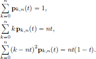
The proof of Weierstrass’s Approximation Theorem can now be completed as follows. For δ > 0, we have
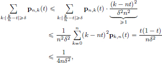
where we used the observation

in order to obtain the last inequality.
Now for δ > 0, set ωδ(x) :=  |x(t) − x(s)|.
Then we have

Let > 0. Since x is uniformly continuous10, we can choose δ > 0 such that ωδ(x) < /2. Next choose n > ||x||∞/(δ2). Then it follows from the above that ||Bnx − x||∞ < , completing the proof of the Weierstrass Approximation Theorem.
Remark 1.2. (Topology). If we look at the collection O of all open sets in a normed space (X, || · ||), we notice that it has the following three properties:
(T1)∅, X ∈ O.
(T2)If Ui ∈ O for all i ∈ I, then  Ui ∈ O.
(T3)If U1, ···, Un is a finite collection of sets from O, then  Ui ∈ O.
More generally, if X is any set (not necessarily a normed space), then any collection O of subsets of X that satisfy properties (T1), (T2), (T3) is called a topology on X and (X, O) is called a topological space. Elements of O are called open sets in (X, O). So for a normed space X, if we take O to be the family of open sets in (X, || · ||), then we obtain a topological space. The following picture displays the hierarchy of structures11.
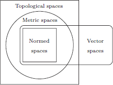
It turns out that one can in fact extend some of the notions from Calculus (such as convergence of sequences and continuity of maps) in the even more general set-up of topological spaces, devoid of any metric or norm, where the notion of closeness is specified by considering arbitrary open neighbourhoods provided by elements of O. In some applications this is exactly the right thing needed, but we will not go into such abstractions here. In fact, this is a very broad subdiscipline of mathematics called Topology.
1.4Sequences in a normed space; Banach spaces
In a normed space, we have a notion of “distance” between vectors, and we can say when two vectors are close by, and when they are far away. So we can talk about convergent sequences. In the same way as in R or C, we can define convergent sequences and Cauchy sequences in a normed space:
Definition 1.6. (Convergent sequence). Let (xn)n∈N be a sequence in X and let L ∈ X. The sequence (xn)n∈N is said to be convergent (in X) with limit L if
In the above, we have used the symbol “∀”, which is read “for every”. Also the symbol “∃” means “there exists a/an”.
Note that the definition says that the convergence of (xn)n∈N to L is the same as the real sequence (||xn − L||)n∈N converging to 0:
that is the distance of the vector xn to the limit L tends to zero, and this matches our geometric intuition. One can show in the same way as with R, that the limit is unique: a convergent sequence has only one limit.
We write  xn = L.
Theorem 1.1. A convergent sequence has a unique limit.
Proof. Let (xn)n∈N be convergent with limits L1 and L2, with L1 ≠ L2. Let := ||L1 − L2||/3 > 0, where the positivity of the follows from the fact that L1 ≠ L2. Since L1 is a limit of the sequence (xn)n∈N, there exists an N1 ∈ N such that for all n > N1, ||xn − L1|| < . Since L2 is a limit of the sequence (xn)n∈N, there exists an N2 ∈ N such that for all n > N2, ||xn − L2|| < . So for n > N1 + N2, we have n > N1 and n > N2, and

So we arrive at the contradiction that 1 < 2/3. Hence our assumption was incorrect, and so a convergent sequence must have a unique limit.
Example 1.18. Consider the sequence (xn)n∈N in the normed space (C[0, 1], || · ||∞), where xn =  , t ∈ [0, 1].
The first few terms of the sequence are shown in the following picture.

From the figure, we see that the terms seem to converge to the zero function. Indeed we have

Given > 0, let N ∈ N be such that N > 1/. Then for all n > N,

So (xn)n∈N is convergent in the normed space (C[0, 1], || · ||∞) to 0.
Definition 1.7. (Cauchy sequence). A sequence (xn)n∈N in a normed space (X, || · ||) is called a Cauchy sequence if for every > 0, there exists an N ∈ N such that for all m, n ∈ N satisfying m, n > N, ||xm − xn|| < .
Roughly speaking, we can make the terms of the sequence arbitrarily close to each other provided we go far enough in the sequence.
Proposition 1.1. Every convergent sequence is Cauchy.
Proof. Let (xn)n∈N be a sequence in (X, || · ||) that converges to L ∈ X. Let > 0. (We want to find N which guarantees for n, m > N that ||xn − xm|| < . But we do know that the terms xn, xm can both be made close to L if n, m are large enough. So we introduce L artificially: ||xn − xm|| = ||xn − L + L − xm|| and use the triangle inequality to complete the argument. The details are given below.)
Then there exists an N ∈ N such that for n > N, we have ||xn − L|| <  .
.
Thus for n, m > N, we have

So the sequence (xn)n∈N is a Cauchy sequence.

We recall from ordinary calculus that in R,

(We will recall the proof of this fact below, in Theorem 1.4 on page 31.) This raises the tempting question of whether this equality is true in general normed spaces too:

If the two sets coincide, then one can conclude that a sequence is convergent by just checking Cauchyness. This is the basis of many existence results in Analysis: for example, the convergence tests in Calculus, the existence results for differential equations, the Riesz representation Theorem12, etc. Once existence is known, (and after showing uniqueness, if valid), one can justify and use numerical approximations. So this prompts the question:
Q. Is it true in all normed spaces that

Answer: No. It is true in some normed spaces, for example

but not true in others, for example

(We will soon justify these claims.)
In light of the above answer, it makes sense to give normed spaces in which

a special name. These are called Banach spaces, after the Polish mathematician Stefan Banach (1892–1945), who laid the foundations of the study of such spaces in his doctoral dissertation from 1920.
Definition 1.8. (Banach space). A normed space in which the set of Cauchy sequences is equal to the set of convergent sequences is called a Banach space. Sometimes, we also call it a complete normed space.
Thus in a complete normed space, or Banach space, the Cauchy condition is sufficient for convergence: the sequence (xn)n∈N converges if and only if it is a Cauchy sequence. So we can determine convergence a priori without the knowledge of the limit. Just as it was possible to introduce new numbers in R as the limits of Cauchy sequences, now in a Banach space, it is possible to show the existence of elements with some property of interest, by making use of the Cauchyness. In this manner, one can sometimes show that certain equations possess a solution. In many cases, one cannot write the solution explicitly. But after existence and uniqueness of the solution is demonstrated, one can do numerical approximations.
(R, | · |) is a Banach space
The completeness of R will be used fundamentally in checking all of our other examples of Banach spaces. While the fact that real Cauchy sequences are always convergent may be familiar to the reader, we reprove this here for the sake of completeness. We will first establish the following elementary lemma, which is valid in all normed space, not just in R.
Lemma 1.3. Every Cauchy sequence in a normed space is bounded13.
Proof. Suppose that (xn)n∈N is a Cauchy sequence in the normed space (X, || · ||). Choose any positive , say = 1. Then there exists an N ∈ N such that for all n, m > N, ||xn − xm|| < . In particular, with m = N + 1 > N, and n > N, ||xn − xN+1|| < . By the Triangle Inequality, for all n > N, ||xn|| = ||xn − xN+1 + xN+1|| ||xn − xN+1|| + ||xN+1|| < 1 + ||xN+1||. On the other hand, for n N, ||xn|| maxt{||x1||, ···, ||xN||, 1 + ||xN+1||} =: M. So ||xn|| M for all n ∈ N, that is, the sequence (xn)n∈N is bounded.
Next we’ll show that:
Theorem 1.2. Every real sequence has a monotone14 subsequence.
Before giving the formal proof, we give an illustration of the idea behind this proof15. If (xn)n∈N is the given sequence, then imagine that there is an infinite chain of hotels along a line, where the nth hotel has height xn, and at the horizon, there is a sea. A hotel is said to have the seaview property if it is higher than all hotels following it (so that from the roof of the hotel, one can view the sea). There are only two possibilities:

Proof. Let (xn)n∈N be a real sequence, and let

(This is the collection of indices of hotels with the seaview property.) Then we have the following two cases.
1°S is infinite.
Arrange the elements of S in increasing order: n1 < n2 < n3 < .... Then (xnk)k∈N is a decreasing subsequence of (xn)n∈N.
2°S is finite.
If S is empty, then define n1 = 1, and otherwise let n1 = max S + 1.
Define inductively nk+1 = min{m ∈ N : m > nk and xm xnk}. (nk+1 is the index of the first hotel blocking the view from the top of the nkth hotel.) The minimum exists as {m ∈ N : m > nk and xm xnk} is a nonempty subset of N. (Otherwise if it were empty, then nk ∈ S, and this is not possible if S was empty, and also impossible if S was not empty, since nk > max S.) Then (xnk)k∈N is an increasing subsequence of (xn)n∈N.
Theorem 1.3.
If a real sequence is monotone and bounded, then it is convergent.
Proof.
1° We will first consider the case of increasing sequences which are bounded. Let (xn)n∈N be an increasing and bounded sequence. We want to show that (xn)n∈N is convergent. But with what limit?

The picture above suggests that the limit should be the smallest number bigger than each of the terms of this sequence, that is, the supremum of the set {xn : n ∈ N}. Since (xn)n∈N is bounded, it follows that the set S := {xn : n ∈ N} has an upper bound and so sup S exists. We show that in fact (xn)n∈N converges to sup S. Let > 0. Since sup S − < sup S, it follows that sup S − is not an upper bound for S, and so there exists an xN ∈ S such that sup S − < xN, that is sup S − xN < . Since (xn)n∈N is an increasing sequence, for n > N, we have xN xn. Since sup S is an upper bound for S, xn sup S and so |xn − sup S| = sup S − xn, Thus for n > N we obtain |xn − sup S| = sup S − xn sup S − xN < .
2° If (xn)n∈N is a decreasing and bounded sequence, then clearly (−xn)n∈N is an increasing sequence. Furthermore if (xn)n∈N is bounded, then (−xn)n∈N is bounded as well (|−xn| = |xn| M). Hence by the case considered above, it follows that (−xn)n∈N is a convergent sequence with limit sup{–xn : n ∈ N} = −inf{xn : n ∈ N} = −inf S, where S = {xn : n ∈ N}. So given > 0, there exists an N ∈ N such that for all n > N, |−xn − (−inf S)| < , that is, |xn − inf S| < . Thus (xn)n∈N is convergent with limit inf S.
Corollary 1.1. (Bolzano-Weierstrass Theorem).
Every bounded real sequence has a convergent subsequence.
Proof. Let (xn)n∈N be a bounded real sequence. The sequence (xn)n∈N has a monotone subsequence, say (xnk)k∈N. Then (xnk)k∈N is bounded too. We have that (xnk)k∈N is monotone and bounded, and hence it is convergent in R.
We are now ready to prove that (R, | · |) is a Banach space.
Theorem 1.4. Every real Cauchy sequence in R is convergent.
Proof. Let (xn)n∈N be Cauchy in R. Then (xn)n∈N is bounded. By the Bolzano-Weierstrass Theorem, (xn)n∈N has a convergent subsequence, say (xnk)k∈N, with limit, say L ∈ R. We will now show that (xn)n∈N is also convergent with limit L. Let > 0. Then there exists an N ∈ N such that for all n, m > N,

Also, since (xnk)k∈N converges to L, we can find an nK > N such that

Thus we have for all n > N that

Thus (xn)n∈N is also convergent with limit L.
Example 1.19. (Q is not complete). Consider the sequence (xn)n∈N in Q defined by x1 = 3/2, and for n > 1, recursively by
Then it can be shown by induction that (xn)n∈N is bounded below by √2, and that (xn)n∈N is monotone decreasing.
(A)xn √2 or all n.
If n = 1, then x1 =  √2 (as
  2). If xn √2 or some n, then

So this gives, since xn+1 0, that xn+1 √2, and the claim follows.
(B)xn xn+1 for all n.
We have

where the last inequality follows from part (A).
So this sequence is convergent in R. Hence it is also Cauchy in R. But as each term xn is a rational number for all n ∈ N, it follows that (xn)n∈N is also Cauchy in Q. However, we now show that (xn)n∈N is not convergent in Q. Suppose, on the contrary, that (xn)n∈N converges to L ∈ Q. Then from the recurrence relation, we obtain using the Algebra of Limits that

and so L2 = 2. As L must be positive (the sequence is bounded below by √2), it follows that L = √2. But this is a contradiction, since we know that there is no rational number whose square is 2.
(Alternately, consider the real number c with the decimal expansion

This number c is irrational because it has a nonterminating and nonrepeating decimal expansion. If we consider the sequence of rational numbers 0.1, 0.101, 0.101001, 0.1010010001, 0.101001000100001, ···, obtained by truncation, then this sequence converges with limit c.)
Example 1.20.
 converges in R, as it is Cauchy: for n > m,

which can be made as small as we please by taking m large enough. We remark that it is not yet known if the limit is rational or irrational!
The completeness of R is the basis for the completeness of other normed spaces, and we’ll see this now.
Finite-dimensional normed spaces are Banach
Theorem 1.5. (Rd, || · ||2) is a Banach space.
Proof.
(Essentially, this is because R is complete, and one has d copies of R in Rd.) Suppose that (xn)n∈N is a Cauchy sequence in Rd; xn = (xn(1), ···, xn(d)). We have  , from which it follows that each of the real sequences (xn(k))n∈N, k = 1, ···, d, is Cauchy in R, and hence convergent, with respective limits, say L(1), ···, L(d) ∈ R. So given > 0, there exists a large enough N such that whenever n > N, we have
  .
.
Set L = (L(1), ···, L(d))∈ Rd.
Then for n > N, ||xn − L||2 =  .
.
Consequently, the sequence (xn)n∈N converges to L.
Corollary 1.2. (C, | · |) is a Banach space.
Proof. This follows from the fact that (R2, || · ||2) is a Banach space.
Exercise 1.27. (∗)16 (Equivalent norms).
Let X be a vector space, and let || · ||a, || · ||b be norms on X. || · ||a is said to be equivalent to || · ||b, denoted by || · ||a ~ || · ||b, if there exist positive constants m and M such that m||x||b ||x||a M ||x||b.
(1)Show that ~ defines an equivalence relation on the set of all norms on X.
(2)Prove for equivalent norms on X, their respective collections of open sets, convergent sequences, and Cauchy sequences coincide.
One can show that all norms are equivalent on Rd as follows. (It follows from here that all finite dimensional normed spaces are Banach since Rd is complete!) In view of the fact that ~ is an equivalence relation, it is enough to show that any norm || · || ~ || · ||2, the Euclidean norm. We do this in three steps:
Step 1. First we will show that there is a positive M such that ||x|| M||x||2 for all x ∈ Rd. Let e1, ···, ed be the standard basis in Rd. Then every x ∈ Rd can be decomposed uniquely as x = x1e1 + ··· + xded, where x1, ···, xd are scalars. So ||x|| = ||x1e1 + ··· + xded|| |x1| ||e1|| + ··· + |xd| ||ed|| (using (N2) and (N3))
Step 2. Let K := {y ∈ Rd : ||y||2 = 1}. Then K is a compact set in the || · ||2 norm topology since it is closed and bounded. The map || · || : K → R is continuous from (K, || · ||2) to (R, | · |): ∀y1, y2 ∈ K, | ||y1|| – ||y2| || ||y1 – y2|| M||y1 – y2||2. By Weierstrass’s Theorem, || · || : K → R attains a minimum value m on K. But this m can’t be zero, since if ||y|| = 0, then y = 0 ∉ K. So this m ought to be positive. Conclusion: ||y|| m for all y’s with ||y||2 = 1.
Step 3. Now we will show that m||x||2 ||x|| for all x ∈ Rn. This is obvious if x = 0, since both sides of the inequality are zero in this case.
If x ≠ 0, then y := x/||x||2 satisfies ||y||2 = 1, so that y ∈ K.
Thus m ||y|| = ||x/||x||2|| = ||x||/||x||2. Rearranging, we obtain m||x||2 ||x||.
So we’ve shown that for all x ∈ Rn, m||x||2 ||x|| M||x||2, that is, || · || ~ || · ||2.
(C[a, b], || · ||∞) is a Banach space
The following theorem is an important result, and lies at the core of several results, for example the result on the existence of solutions for Ordinary Differential Equations (ODEs).
Theorem 1.6. (C[a, b], || · ||∞) is a Banach space.
Proof. The idea behind the proof is similar to the proof of the completeness of Rd. If (xn)n∈N is a Cauchy sequence, then we think of the xn(t) as being the “components” of xn indexed by t ∈ [a, b]. We first freeze a t ∈ [a, b], and show that (xn(t))n∈N is a Cauchy sequence in R, and hence convergent to a number (which depends on t), and which we denote by x(t). Next we show that the function t x(t) is continuous, and finally that (xn)n∈N does converge to x in the supremum norm.

Let (xn)n∈N be a Cauchy sequence. Let t ∈ [a, b]. We claim that (xn(t))n∈N is a Cauchy sequence in R. Let > 0. Then there exists an N ∈ N such that for all n, m > N, ||xn − xm||∞ < . But

for n, m > N. This shows that indeed (xn(t))n∈N is a Cauchy sequence in R. But R is complete, and so the Cauchy sequence (xn(t))n∈N is in fact convergent, with a limit which depends on which t ∈ [a, b] we had frozen at the outset. To highlight this dependence on t, we denote the limit of (xn(t))n∈N by x(t). (Thus for example x(a) is the number which is the limit of the convergent sequence (xn(a))n∈N, x(b) is the number which is the limit of the convergent sequence (xn(b))n∈N, and so on.) So we have a function

We call this function x. This will serve as the limit of the sequence (xn)n∈N. But first we have to see if it belongs to C[a, b], that is, we need to check that this x is continuous on [a, b].
Let t ∈ [a, b]. We will show that x is continuous at t. Recall that in order to do this, we have to show that for each > 0, there exists a δ > 0 such that whenever |τ − t| < δ, we have |x(τ) – x(t)| < . Let > 0.
Choose N large enough so that for all n, m > N, ||xn − xm||∞ < /3.
Let τ ∈ [a, b]. Then for n > N, |xn(τ) – xN+1(τ)| ||xn − xN+1||∞ < /3.
Now let n → ∞: |x(τ) – xN+1(τ)| =  |xn(τ) – xN+1(τ)| /3.
The choice of τ ∈ [a, b] was arbitrary, and so for all τ ∈ [a, b]

Now xN+1 ∈ C[a, b]. So there exists a δ > 0 such that whenever |τ − t| < δ,

Thus whenever |τ − t| < δ, we have

This shows that x is continuous at t. As the choice of t ∈ [a, b] was arbitrary, x is continuous on [a, b].
Finally, we show that (xn)n∈N does converge to x. Let > 0. Choose N large enough so that for all n, m > N, ||xn − xm||∞ < . Fix n > N. Let t ∈ [a, b]. Then for all m > N, |xn(t) − xm(t)| ||xn − xm||∞ < . Thus

But t ∈ [a, b] was arbitrary. Hence ||xn − x||∞ =  |xn(t) − x(t)| .
But we could have fixed any n > N at the outset and obtained the same result. So for all n > N, ||xn – x||∞ . Thus  xn = x in (C[a, b], || · ||∞).
This completes the proof.
Example 1.21. (C[a, b] is not a a Banach space with the || · ||2-norm.)
We will work with [a, b] = [0, 2] for computational ease. Consider the sequence (xn)n∈N in C[0, 2], where xn has a graph as shown below.

(xn)n∈N is a Cauchy sequence in (C[0, 2], || · ||2): indeed, for n > m,

Suppose that (xn)n∈N converges to x ∈ C[0, 2] in (C[0, 2], || · ||2). Then:
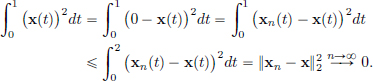
As x ∈ C[0, 1],  implies that x(t) = 0 for t ∈ [0, 1].

Let N ∈ N. Then for all n > N,

and so 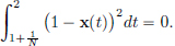 As x ∈ C[1 +
  , 2], this implies

Since N ∈ N was arbitrary, it follows that x(t) = 1 for all t ∈ (0, 1].
Conclusion:
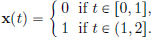
But then x ∉ C[0, 2] (as it has a discontinuity at t = 1), a contradiction.
The following is an instance where one uses “Cauchyness  convergence” in Banach spaces.
Theorem 1.7. In a Banach space, absolutely convergent series converge, that is:
If(xn)n∈N is a sequence in a Banach space(X, || · ||) such that  < ∞, then
  converges in X. Moreover,
Proof. Let sn = x1 + ··· + xn, n ∈ N. We want to show that converges, that is, the sequence (sn)n∈N of partial sums converges in X.
As X is a Banach space, it is enough to show that (sn)n∈N is Cauchy.
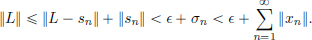
We are given that the real series converges, that is its sequence (σn)n∈N of partial sums converges, where σn = ||x1|| + ··· + ||xn||, n ∈ N.
In particular, (σn)n∈N is Cauchy. For n > m,

and this can be made as small as we please for all n > m > N with a large enough N. (The rightmost equality above follows from the leftmost inequality.) Thus (sn)n∈N is Cauchy in X, and hence convergent in X (as X is a Banach space), to, say, L ∈ X. Let > 0. Then there exists an n such that ||sn − L|| < . Thus
As the choice of > 0 was arbitrary, 
Example 1.22.  converges in (C[0, 2π], || · ||∞).
(Here sin(n·) means the function t sin(nt) : [0, 2π] → R.)
Indeed, we have  and
and 
So 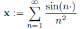 defines a continuous function on [0, 2π].
We can get a good idea of the limit by computing the first N terms (with a large enough N) and plotting the resulting function; the error can then be bounded as follows:

For example, if N = 100, then the error is bounded above by

Using Maple, we have plotted the partial sum of x with N = 100.
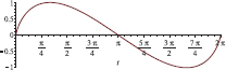
Thus the sum converges to a continuous function that lies in the strip of width 0.01 around the graph shown in the figure.
Later on, we will use this theorem to show that eA converges, where A belongs to CL(X). Here CL(X) denotes a certain Banach space, namely the space of all “continuous linear transformations” from X to itself, with the “operator norm”. For example, when X = Rd, CL(X) turns out to be the space of all square d × d real matrices. Why fuss over eA? The answer is that it plays a role in differential equations: the initial value problem

has the unique solution x(t) = etAx0, t ∈ R.
Also, using the fact that (C[a, b], || · ||∞) is a Banach space, one can show the Fundamental Theorem of Ordinary Differential Equations (ODEs):
Theorem 1.8. (Existence and Uniqueness of ODEs).
If there exists an r > 0 and an L > 0 such that f : R × R → R satisfies

then for all x0 ∈ R, there exists a T > 0 and there exists an x ∈ C1[0, T] solving the Initial Value Problem

on [0, T], and moreover (IVP) has a unique solution.
Condition (L) on f is expressed as: f is “Lipschitz in x, uniformly in t”.
Proof. (Uniqueness) Let x1, x2 be two solutions to (IVP) on [0, T] for some T > 0. Let 

Then

So 
Let17  and
and 
Note that  . Then for all
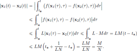
Thus

and so  , that is, N 1, a contradiction. This shows the uniqueness.
(Existence) We will write down a sequence of recursively defined functions, which are not solutions, but serve as “good approximations”:
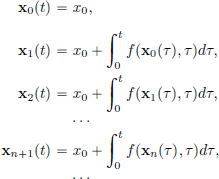
We will show that (xn)n0 converges to x in 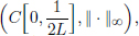 and this x solves (IVP)! (So, in particular, we’ll take
  .)
.)
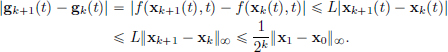
We note that xn+1 = 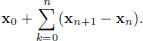
Also, for 0 t  ,
,
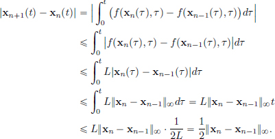
Thus 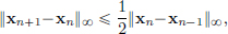 and so
  .
.
Hence 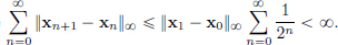
So  converges in (C[0, T], || · ||∞), to, say, x ∈ C[0, T].
We know that 
Passing the limit as n → ∞, we have (see the explanation below):

(Here’s the justification. Define the continuous gn(n = 0, 1, 2, 3, ···) by:

Then the sequence g0, g1, g2, ··· is the sequence of partial sums of the series

We have
So (1.12) converges absolutely to some g in (C[0, T], || · ||∞). We have

We’ll now use the fact that if  converges to f in (C[a, b], || · ||∞), then

and this is precisely the content of Exercise 2.14 on page 73, which will be dealt with after discussing continuity of linear transformations. Using this,

that is, we have proved (1.11).)
Thus x(0) = x0 + 0 = x0, and by the Fundamental Theorem of Calculus, x′(t) = 0 + f(x(t), t) for all t ∈ [0, T].
Exercise 1.28. (Nonuniqueness when non-Lipschitz).
(1)Let f(x) :=  , x ∈ R. Show that f is not Lipschitz, that is, there is no constant L > 0 such that for all x, y ∈ R, |f(x) − f(y)| L|x − y|.
(2)Check that x1  0 and x2(t) = t2/4 are solutions to the Initial Value Problem
(ℓp, || ·||p) are Banach spaces
Theorem 1.9. Let 1 p +∞. Then(ℓp, || · ||p) is a Banach space.
Proof. We had already seen that ℓp is a vector space, and the fact that || · ||p defines a norm will be established in Exercise 1.35 (page 44). We must now show that ℓp is complete. Let (xn)n∈N be a Cauchy sequence in ℓp. Denote the kth term of xn by  . The proof will be carried out in 3 steps.
Step 1. We have 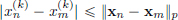 and so
  is a Cauchy sequence in K (= R or C), and consequently, it is convergent, with limit, say, x(k). Set x = (x(k))k∈N.
Step 2. We show that x belongs to ℓp. Let > 0. Then there exists an N ∈ N such that for all n, m > N, ||xn − xm||p < . Fix any n > N.
If K ∈ N, then for p < ∞, 
Passing the limit as m goes to ∞ yields 
As the choice of K was arbitrary,

So xn − x belongs to ℓp. But xn ∈ ℓp. Hence (x − xn) + xn = x ∈ ℓp too. The p = ∞ case can be seen as follows. Fix n > N and k ∈ N. Then for all m > N,  . Passing the limit as m goes to ∞ yields
  . As k was arbitrary,

that is, xn − x belongs to ℓ∞. As xn ∈ ℓ∞, it now follows that x ∈ ℓ∞ too.
Step 3. Finally, we’ll show that (xn)n∈N converges to x. In the case when p < ∞, proceeding as in Step 2, (1.13) gives for all n > N, ||xn − x||p .
When p = ∞, (1.14) gives ||xn − x||∞ for all n > N.
Exercise 1.29. (Characterisation of closed sets).
Let X be a normed space and F be a subset of X. Show that the following two statements are equivalent:
(1)F is closed.
(2)For every sequence (xn)n∈N in F ( n ∈ N, xn ∈ F), which is convergent in X with limit x ∈ X, we have that x ∈ F.
Exercise 1.30. Show that c00, the set of all sequences with compact support (that is sequences which have all terms equal to zero eventually), is a subspace of ℓ2 which is not closed.
Exercise 1.31. (Closure of a set).
Let X be a normed space and S be a subset of X. A point L ∈ X is a limit point of S if there exists a sequence (xn)n∈N in S\{L} with limit L. The set consisting of all points and limit points of S is denoted by S, and is called the closure of S.
(1)Prove that S is the smallest closed set which contains S.
(2)Show that if Y is a subspace of X, then Y is also a subspace of X.
(3)Prove that if C is a convex subset of X, then C is also convex.
(4)Show that a subset D of X is dense if and only if D = X.
Exercise 1.32. Show that ℓ1  ℓ2.
ℓ2.
Is ℓ1 a Banach space with the topology induced from ℓ2?
Exercise 1.33. Let c0 be the set if all sequences convergent with limit 0. Then c0 is a subspace of the normed space ℓ∞. Prove that c0 is a Banach space.
Exercise 1.34. Let (X, || · ||) be a normed space, and let (xn)n∈N be a convergent sequence in X with limit x. Prove that (||xn||)n∈N is a convergent sequence in R and that  .
.
Exercise 1.35. Show that if 1 p ∞, then ℓp is a normed space.
Exercise 1.36. Show that (C1[a, b], || · ||1,∞) is a Banach space.
Exercise 1.37. (∗) We have seen that if X is a Banach space, then every absolutely convergent series is convergent. The aim of this exercise is to show the converse. That is, prove that if X is a normed space with the property that every absolutely convergent series converges, then X is a Banach space. Hint: Construct a subsequence (xnk)k∈N of a given Cauchy sequence (xn)n∈N possessing the property that if n > nk, then ||xn − xnk|| < 1/2k. Define u1 = xn1, uk+1 =xnk+1 − xnk, k ∈ N, and consider the series with terms uk.
Exercise 1.38. (Finite product of normed spaces).
If X, Y are normed spaces, then X × Y is a vector space with component-wise operations. Show that ||(x, y)|| := max{||x||, ||y||}, (x, y) ∈ X × Y, defines a norm on X × Y. Prove that if X, Y are Banach, then so is X × Y.
1.5Compact sets
In this section, we study an important class of subsets of a normed space, called compact sets. Before we learn the definition, let us give some motivation for this concept.
Of the different types of intervals in R, perhaps the most important are those of the form [a, b], where a, b are finite real numbers. Why are such intervals so important? We know of an important result, the Extreme Value Theorem18 , where such intervals play a vital role. recall that the Extreme Value Theorem asserts that any continuous function f : [a, b] → R attains a maximum and a minimum value on [a, b]. This result does not hold in general for continuous functions f : I → R with I = (a, b) or I = [a, b) or I = (a, ∞), and so on. Besides its theoretical importance in Analysis, the Extreme Value Theorem is also a fundamental result in Optimisation Theory. It turns out that when we want to generalise this result, the notion of “compact sets” is pertinent, and later on, we will learn the following analogue of the Extreme Value Theorem: If K is a compact subset of a normed space X and f : K → R is continuous, then f assumes a maximum and a minimum on K. Here is the definition of a compact set.
Definition 1.9. (Compact set). Let (X, || · ||) be a normed space. A subset K of X is said to be compact if every sequence in K has a convergent subsequence with limit in K, that is, if (xn)n∈N is a sequence such that xn ∈ K for each n ∈ N, then there exists a subsequence (xnk)k∈N which converges to some L ∈ K.
Example 1.23. (Compact intervals in R). The interval [a, b] is a compact subset of R. Indeed, every sequence (an)n∈N contained in [a, b] is bounded, and thus by the Bolzano-Weierstrass Theorem, possesses a convergent subsequence, say (ank)k∈N, with limit L. But since a ank b, for all k’s, by letting k → ∞, we obtain a L b, that is, L ∈ [a, b]. Hence [a, b] is compact.
On the other hand, (a, b) is not compact, since the sequence

is contained in (a, b), but it has no convergent subsequence whose limit belongs to (a, b). Indeed this is because the sequence is convergent, with limit a, and so every subsequence of this sequence is also convergent with limit a, which doesn’t belong to (a, b).
R is not compact since the sequence (n)n∈N cannot have a convergent subsequence. Indeed, if such a convergent subsequence existed, it would also be Cauchy, but the distance between any two distinct terms, being distinct integers, is at least 1, contradicting the Cauchyness.
In the above list of nonexamples, note that R is not bounded, and that (a, b) is not closed. On the other hand, in the example [a, b], we see that [a, b] is both bounded and closed. It turns out that in Rd, having the property “closed and bounded” is a characterisation of compact sets, and we will show this below.
Theorem 1.10.
A subset K of Rd is compact if and only if K is closed and bounded.
Before showing this, we prove a technical result, which besides being interesting on its own, will also somewhat simplify the proof of the above theorem.
Lemma 1.4. Every bounded sequence in Rd has convergent subsequence.
Proof. As all norms on Rd are equivalent, it suffices to work with the || · ||2 norm. We prove this using induction on d. Let us consider the case when d = 1. Then the statement is precisely the Bolzano-Weierstrass Theorem!
Suppose that the result has been proved in Rd for a d 1. We’ll show that it holds in Rd+1. Let (xn)n∈N be a bounded sequence. We split each xn into its first d components and its last component in R, and write xn = (αn, βn), where αn ∈ Rd and βn ∈ R. Since  we see that (αn)n∈N is a bounded sequence in Rd. By the induction hypothesis, it has a convergent subsequence, say (αnk)k∈N which converges to, say α ∈ Rd. Now consider the sequence (βnk)k∈N in R. Then (βnk)k∈N is bounded, and so by the Bolzano-Weierstrass Theorem, it has a convergent subsequence (βnkℓ)ℓ∈N, with limit, say β ∈ R. Then we have

So the bounded sequence (xn)n∈N has (xnkℓ)ℓ∈N as a convergent subsequence.
Also, we note that the “only if ” part of Theorem 1.10 holds in all normed spaces.
Proposition 1.2. Let(X, || · ||) be a normed space, and K ⊂ X be compact. Then K must be closed and bounded.
Proof.
(K is closed:) Let (xn)n∈N be a sequence in K that converges to L. Then there is a convergent subsequence, say (xnk)k∈N that is convergent to a limit L′ ∈ K. But as (xnk)k∈N is a subsequence of a convergent sequence with limit L, it is also convergent to L. By the uniqueness of limits, L = L′ ∈ K. Thus K is closed.
(K is bounded:) Suppose that K is not bounded. Then given any n ∈ N, we can find an xn ∈ K such that ||xn} > n. But this implies that no subsequence of (xn)n∈N is bounded. So no subsequence of (xn)n∈N can be convergent either. This contradicts the compactness of K. Thus our assumption was incorrect, that is, K is bounded.
Now we return to the task of proving of Theorem 1.10.
Proof. It remains to just prove the “if ” part. Let K be closed and bounded. Let (xn)n∈N be a sequence in K. Then (xn)n∈N is bounded, and so it has a convergent subsequence, with limit L. But since K is closed and since each term of the sequence belongs to K, it follows that L ∈ K. Consequently, K is compact.
Example 1.24. If a, b ∈ R and a < b, then the intervals (a, b], [a, b) are not compact in R, since although they are bounded, they are not closed.
The intervals (−∞, b], [a, ∞) are not compact, since although they are closed, they are not bounded.
Let us consider an interesting compact subset of the real line, called the Cantor set.
Example 1.25. (Cantor set). The Cantor set is constructed as follows. Let F1 := [0, 1], and delete from F1 the open interval  which is its middle third, and denote the remaining set by F2. Thus we have that
  Next, delete from F2 the middle thirds of its two pieces, namely the open intervals
  and
and  and denote the remaining set by F3. It can be checked that
  Continuing this process, that is, at each stage deleting the open middle third of each interval remaining from the previous stage, we obtain a sequence of sets Fn, each of which contains all of its successors.

The Cantor set is defined by 
C is contained in [0, 1], and consists of those points in the interval [0, 1] which “ultimately remain” after the removal of all the open intervals  What points do remain? C clearly contains the end-points of the intervals which make up each set Fn:

Does C contain any other points? Actually, C contains many more points than the above list of end points. After all, the above list of endpoints is countable, but it can be shown that C is uncountable, see Example 7.1 on page 362.
As C is an intersection of closed sets, it is closed. Moreover it is contained in [0, 1] and so it is also bounded. Consequently it is compact. (It turns out that the Cantor set is a very intricate mathematical object, and is often a source of interesting examples/counterexamples in Analysis. For example, it can be shown that the Lebesgue measure of C is 0, and so C is an example of an uncountable set with Lebesgue measure 0; see Example 7.1 on page 362.)
Remark 1.3. Since all norms on a finite dimensional normed space are equivalent, we have the following consequence of Theorem 1.10.
Corollary 1.3. Let X be a finite dimensional normed space.
A subset K ⊂ X is compact if and only if K is closed and bounded.
However, in infinite dimensional normed spaces, although compact sets continue to be necessarily closed and bounded, it turns out that closed and bounded sets may fail to be compact. We give two examples below, the closed unit ball in ℓ2 (Example 1.26) and in C[0, 1] (Example 1.28).
Example 1.26. (The closed unit ball in ℓ2 is not compact.)
Consider the closed unit ball with centre 0 in the normed space ℓ2:
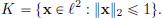
Then K is bounded, it is closed (since its complement is easily seen to be open), but K is not compact, as shown below.
For example, take the sequence (en)n∈N, where en is the sequence with only the nth term equal to 1, and all other terms are equal to 0:

Then this sequence (en)n∈N in K ⊂ ℓ2 can have no convergent subsequence. Indeed, whenever n ≠ m, ||en − em||2 =  , and so any subsequence of (en)n∈N must be non-Cauchy, and hence also not convergent!
Example 1.27. (∗)(The Hilbert cube in ℓ2 is compact.)
Let C denote the set of all real sequences (xn)n∈N, whose nth term satisfies 0 xn 1/n for all n ∈ N. Then it is clear that C is a subset of the real vector space ℓ2. It can be shown that C is a compact subset of ℓ2, and we include a proof below, even though it is somewhat technical. The proof relies on creating subsequences of subsequences, and eventually using a “diagonal” sequence created in this process. We will also use a similar process in the proof of Theorem 5.4 (page 213) in Chapter 5. If the reader so wishes, he/she can skip the proof below for now, and move on to Example 1.28.
Let (xm)m∈N be a sequence in C. The task is to produce a subsequence of this sequence which converges in ℓ2 to an x in C. Let  Then for all n and m,
In particular,  and as [0, 1] is compact, there is a subsequence m1(1), m1(2), m1(3), ··· of 1, 2, 3, ··· such that
  is convergent, with limit, say, x(1) ∈ [0, 1].
Now  and as [0, 1/2] is compact, there is a subsequence (m2(j))j2 of (m1(j))j2 such that
  is convergent, with limit, say, x(2) ∈ [0, 1/2].
Proceeding in this manner, we get for all ℓ that there is a subsequence (mℓ(j))jℓ of (mℓ−1(j))jℓ such that  is convergent, with limit x(ℓ) ∈ [0, 1/ℓ]. We claim that
  converges in ℓ2 to the sequence
  . See the schematic diagram below.

First, let us note that x ∈ C because for all n ∈ N, 0 x(n) 1/n.
Now the plan is to show that ||xmj(j) − x||2 is small for all js sufficiently large. To do this, we will split this quantity into two parts, and estimate them separately:

Let us see how to handle the second summand on the right-hand side above.
Let > 0. Let N be such that  Then we have

Having accomplished this, let us now estimate the first summand in (1.15).
For all  . As (mj(j))jN is a subsequence of (mN(j))jN, and hence also of each (mn(j))jn for n N, it follows that for all
So we can find a J such that for all  Thus
Thus

As > 0 was arbitrary, we have indeed shown that (xmj(j))j∈N converges in ℓ2 to x ∈ C. This completes the proof of the compactness of the Hilbert cube C.
Example 1.28. (The closed unit ball in (C[0, 1], || · ||∞) is not compact.) Consider the closed unit ball with centre 0 in (C[0, 1], || · ||∞):

Then K is bounded, and also it is closed (since its complement is open). But K is not compact, and this can be demonstrated by considering the sequence (xn)n∈N, where the graphs of the xns have “narrowing” tents of height 1, with the supports of the tents moving to the right, on half of each remaining interval, as shown in the following picture:

Then this sequence does not have a convergent subsequence, since if it did, then the convergent subsequence would be Cauchy, but whenever n ≠ m, ||xn − xm||∞ = 1, a contradiction to the Cauchyness.
Exercise 1.39. Let K be a compact subset of Rd (with the Euclidean norm || · ||2), and F ⊂ Rd be a closed subset. Show that F K is compact in Rd.
Exercise 1.40. Show that the unit sphere Sd−1 := {x ∈ Rd : ||x||2 = 1} with centre 0 in Rd, is compact in Rd.
Exercise 1.41. (∗)
Consider the normed space (R2×2, || · ||∞) from Exercise 1.13, page 17.
(1)Show that the set O(2) := {R ∈ R2×2 : R R = I} of orthogonal matrices is a compact set.
(2)Is the indefinite orthogonal group O(1, 1) := {R ∈ R2×2 : R JR = J},
where  also compact?
Hint: Consider “hyperbolic rotations” 
Exercise 1.42. Show that  is compact in R.
Remark 1.4. (Definition of compactness.) The notion of a compact set that we have defined is really sequential compactness. In the context of the more general topological spaces, one defines the notion of compactness as follows.
Definition 1.10. Let X be a topological space with the topology given by the family of open sets O. Let K ⊂ X. A collection C = {Ui : i ∈ I} of open sets is said to be an open cover of K if 
K ⊂ X is said to be a compact set if every open cover of K has a finite subcover, that is, given any open cover C = {Ui : i ∈ I} of K, there exist finitely many indices i1, ···, in ∈ I such that K ⊂ Ui1 ··· Uin.
In the case of normed spaces, it can be shown that the set of compact sets coincides with the set of sequentially compact sets. But in general topological spaces, these two notions may not be the same; see for instance [Steen and Seebach (1995)].