Mathematical Logic

THE PROPOSITIONAL CALCULUS

§ 1. Linguistic considerations: formulas. Mathematical logic (also called symbolic logic) is logic treated by mathematical methods. But our title has a double meaning, since we shall be studying the logic that is used in mathematics.

Logic has the important function of saying what follows from what. Every development of mathematics makes use of logic. A familiar example is the presentation of geometry in Euclid’s “Elements” (c. 330-320 B.C.), in which theorems are deduced by logic from axioms (or postulates). But any orderly arrangement of the content of mathematics would exhibit logical connections. Similarly, logic is used in organizing scientific knowledge, and as a tool of reasoning and argumentation in daily life.

Now we are proposing to study logic, and indeed by mathematical methods. Here we are confronted by a bit of a paradox. For, how can we treat logic mathematically (or in any systematic way) without using logic in the treatment?

The solution of this paradox is simple, though it will take some time before we can appreciate fully how it works. We simply put the logic that we are studying into one compartment, and the logic that we are using to study it in another. Instead of “compartments”, we can speak of “languages”. When we are studying logic, the logic we are studying will pertain to one language, which we call the object language, because this language (including its logic) is an object of our study. Our study of this language and its logic, including our use of logic in carrying out the study, we regard as taking place in another language, which we call the observer’s language.¹ Or we may speak of the object logic and the observer’s logic.

It will be very important as we proceed to keep in mind this distinction between the logic we are studying (the object logic) and our use of logic in studying it (the observer’s logic). To any student who is not ready to do so, we suggest that he close the book now, and pick some other subject instead, such as acrostics or beekeeping.

All of logic, like all of physics or all of history, constitutes a very rich and varied discipline. We follow the usual strategy for approaching such disciplines, by picking a small and manageable portion to treat first, after which we can extend our treatment to include some more.

The portion of logic we study first deals with connections between propositions which depend only on how some propositions are constructed out of other propositions that are employed intact, as building blocks, in the construction. This part of logic is called propositional logic or the propositional calculus.

We deal with propositions through declarative sentences which express them is some language (the object language); the propositions are the meanings of the sentences.² Declarative sentences express propositions (while interrogatory sentences ask questions and imperative sentences express commands). The same proposition may be expressed by different (declarative) sentences. Thus “John loves Jane” and “Jane is loved by John” express the same proposition, but “John loves Mary” expresses a different proposition. Under the usual definition of > from <, the two sentences “5 < 3” and “3 > 5” express the same proposition (which happens to be false), namely that increasing 5 by a suitable positive quantity will give 3; but “5² — 4² = 10” expresses a different proposition (also false). Each of “5 < 3”, “3 > 5” and “5² – 4² = 10” asserts something about the outcome of a mathematical process, which is the same process in the first two cases, but a different one in the third. “3 — 2 = 1” and “(481 — 581) + 101 = 1” express two different propositions (both true).

We save time, and retain flexibility for the applications, by not now describing any particular object language. (Examples will be given later.)

Throughout this chapter, we shall simply assume that we are dealing with one or another object language in which there is a class of (declarative) sentences, consisting of certain sentences (the aforementioned building blocks) and all the further sentences that can be built from them by certain operations, as we describe next. These sentences we call formulas, in deference to the use of mathematical symbolism in them or at least in our names for them.

First, in this language there are to be some unambiguously constituted sentences, whose internal structure we shall ignore (for our study of the propositional calculus) except for the purpose of identifying the sentences.

We call these sentences prime formulas or atoms; and we denote them by capital Roman letters from late in the alphabet, as “P”, “Q”, “R”, . . . , “P₁”, “P₂”, “P₃”, . . .. Distinct such letters shall represent distinct atoms, each of which is to retain its identity throughout any particular investigation in the propositional calculus.

Second, the language is to provide five particular constructions or operations for building new sentences from given sentences. Starting with the prime formulas or atoms, we can use these operations, over and over again, to build other sentences, called composite formulas or molecules, as follows. (The prime formulas and the composite formulas together constitute the formulas.,)³ If each of A and B is a given formula (i.e. either a prime formula, or a composite formula already constructed), then , A⊃B, A & B and A ∨ B are (composite) formulas. If A is a given formula, then is a (composite) formula. (The first four operations are “binary” operations, the last is “unary”.)

The symbols “”, “⊃”, “&”, “∨” and “” are called propositional connectives⁴ They can be read by using the words shown at the right in the following table; but the symbols are easier to write and manipulate.⁵

Here we must mention the fact that the natural word languages, such as English, suffer from ambiguities. (Of this, more will be said later.) Logicians are therefore prone to build special symbolic languages. Our unspecified object language may be such a symbolic language, having symbols “”, “⊃”, “&”, “∨” and “” which play roles described accurately below but suggested or approximately described by the words. It comes to nearly the same thing to think of the object language as a suitably restricted and regulated part of a natural language, such as English; then “”, “⊃”, “&”, ∨ and “ ” can be thought of as names in the observer’s language for the verbal expressions at the right in the table.⁶

The names at the left in the table above apply to the propositional connectives or to the formulas constructed using them. Thus “&” is our symbol for conjunction; and A & B is a conjunction, namely the conjunction of A and B. Also A ⊃ B is the implication by A of B; etc.

So that there will be no ambiguity as to which formulas are the atoms, we now stipulate that none of the atoms be of any of the five forms , A ⊃ B, A & B, A ∨ B and which the molecules have.⁷ For example, “Socrates is a man”, “John loves Jane”, “John loves Mary”, “5 < 3”, “3 > 5”, “a+b = c” and “a > 0” (where “a”, “b”, “c” stand for numbers) could be atoms; then “John loves Jane or John loves Mary”, “ 5 < 3” and “5 < 3 3 > 5” would be molecules.

We are using capital Roman letters from the beginning of the alphabet, as “A”, “B”, “C”, . . . , “A₁”, “A₂”, “A₃”, . . . , to stand for any formulas, not necessarily prime. Distinct such letters “A”, “B”, “C”, . . . , “A₁”, “A₂”, “A₃”, . . . need not represent distinct formulas (in contrast to “P”, “Q”, “R”, “P₁”, “P₂”, “P₃”, . . . , which represent distinct prime formulas).

Composite formulas would sometimes be ambiguous as to the manner in which the symbols are to be associated if we did not introduce parentheses. So we shall write “(A⊃B) ⊃ C” or “A⊃(B ⊃ C)” and not simply “A⊃ B⊃ C”. However we can minimize the need for parentheses by assigning decreasing ranks to our propositional connectives, in the order listed:⁸

Where there would otherwise be two ways of construing a formula, the connective with the greater rank reaches further. Thus “A⊃B& C” shall mean A ⊃ (B & C), and “ ”shall mean . The unary operator being ranked last, “ ” shall mean rather than and “ ” shall mean . This practice is familiar in algebra, where “a + bc² = d” means (a + (b(c²))) = d.

EXAMPLE 1. In “A ⊃(B⊃ C)” the letters “A”, “B”, “C” stand for formulas constructed from P, Q, R, . . . , P₁ P₂, P₃, . . . (i.e. from the atoms named by “P”, “Q”, “R”, . . . , “P₁”, “P₂”, “P₃”) using (zero or more times) , and (as required) parentheses. For example, A ⊃(B⊃ C) might be the particular formula (so A is P, B is Q ∨ R and C is ). Here a second pair of parentheses has been inserted, but our ranking of the symbols makes parentheses around Q ∨ R superfluous. The parentheses enable us to see how the formula was constructed, starting from the atoms P, Q, R, and using five steps of composition to introduce the five numbered occurrences of propositional connectives, thus :

In a manner obvious from the parentheses or the construction, each occurrence of a connective “connects” or “applies to” or “operates on” one or two parts of the formula, called the scope of that (occurrence of a) connective. The scopes of the connectives are shown here by correspondingly numbered underlines; thus the scope of ⊃₄ consists of the two parts Q ∨ R and .

EXERCISE 1.1. Identify the scope of each (occurrence of a) propositional connective: (a) . (b).

§ 2. Model theory: truth tables, validity. Not only are we restricting ourselves in this chapter to the study of the logic of propositions. But also in this and later chapters we shall concern ourselves primarily with a certain kind of logic, called classical logic.

Since the discovery of non-Euclidean geometries by Lobatchevsky (1829) and Bolyai (1833), it has been clear that different systems of geometry are conceptually equally possible. (We shall say a little more about this in § 36.) Similarly, there are different systems of logic. Different theories can be deduced from the same mathematical postulates, the differences depending on the system of logic used to make the deductions. The classical logic, like the Euclidean geometry, is the simplest and the most commonly used in mathematics, science and daily life. In this book we shall find the space for only brief indications of other kinds of logic.⁹

Thus far we have assumed about each prime formula or atom only that it can be identified; i.e. that each time it occurs it can be recognized as the same, and as different from other atoms.

Now we make one further assumption about the atoms, which is characteristic of classical logic. We assume that each atom (or the proposition it expresses) is either true or false but not both.

We are not assuming that we know of each atom whether it is true or false. That knowledge would require us to look into the constitution of the atoms, or to consider facts to which they allude under an agreed interpretation of the words or symbols, none of which is within our purview in the propositional calculus.

Our assumption is thus that, for each atom, there are exactly two possibilities: it may be true, it may be false.

The question now arises: How does the truth or falsity (truth value) of a composite formula or molecule depend upon the truth value(s) of its component prime formula(s) or atom(s)? This will be determined by repeated use of five definitions, given by the following tables. These tables relate the truth value of each molecule to the truth value(s) of its immediate component(s). In the left-hand columns we list all the possible assignments of truth and falsity to the immediate component(s). Then in the line (or row) for a given assignment, we show the resulting truth value of each molecule in the column headed by that molecule.

Thus is true exactly when A and B have the same truth value (hence the reading “equivalent’’, i.e. “equal valued”, for ); A⊃B is false exactly when A is true and B is false; A & B is true exactly when A and B are both true; A ∨ B is false exactly when both are false; and is true exactly when A is false.

Some controversy has arisen about the name “implication”, and the reading “implies”, for our ⊃. Say A is “the moon is made of green cheese” and B is “2+2=5”. Then A⊃B is true under our table (because A is false), even though there is no connection of ideas between A and B. Similarly, if B is “2+2=4”, A⊃B is true (because B is true), quite apart from whether A bears any relationship to “2+2=4”. This is considered paradoxical by some writers (Lewis 1912,1917, Lewis and Langford 1932).¹⁰

In modern mathematics the name “multiplication” is often used for various mathematical operations that behave more or less analogously to the arithmetical one called “multiplication”. Similarly, we find it convenient to use the name “implication” to designate the operation defined by the second truth table above; and then in our logical discussions we usually read A ⊃ B as “A implies B”, even though “if A then B” or “A only if B” probably renders the meaning better in everyday English. This “implication”, and the present “equivalence”, are called more specifically “material implication” and “material equivalence”.¹¹

It is, of course, possible to be interested in other senses of “implication”; but then one must have recourse to ways of defining it other than by a “two-valued truth table”. Our definition is the only reasonable one with such a table.¹²

A related question is why we should want to assert a material implication A⊃B, when if A is true we could more simply assert B (or if our hearers don’t know that A is true, we could more informatively assert A & B), and if A is false we could more simply say nothing. But we ordinarily assert sentences of the form “If A, then B” when we don’t know whether A is true or not. For example, before an election I might say [1] “If our candidate for President carries the state by 500,000, then our man for the Senate will also win”. This form of statement enables me to predict what will happen in one eventuality without attempting to say more. If it turns out that our candidate for President doesn’t carry the state by 500,000, my prediction will not have been proved false. Since we are committed here to a two-valued logic, my statement should then be regarded as true, though perhaps uninteresting. If when I speak, returns are in showing our candidate ahead by a safe 500,000, I would more likely say [la] “Our man for the Senate will win” or [lb] “Since our candidate for President is carrying the state by 500,000, our man for the Senate will win”. But [1] would not have become false, just partially redundant and thus unnatural for me to say (unless I haven’t heard the latest election returns).

To take an analogous mathematical example, suppose a positive integer n > 1 is written on a piece of paper in your pocket, and I do not know what the integer is. I could truthfully say [2] “If n is odd, then xⁿ + yⁿ can be factored”. By saying this, I am claiming that, when you produce the paper showing the value of n, then I will be able to factor xⁿ + yⁿ for the n you produce if it turns out to be odd (and I am making no claim about the factorability of xⁿ + yⁿ in the contrary case). Thus, if you have bet that I am wrong, to settle the bet you produce the number n. If for example it is 3, I then show you the factorization (x + y)(x² — xy + y²), and you pay me. If for example it is 4 (or 6), I win automatically.

These examples should make it clear that material implication A⊃B (“If A, then B”) is a useful and natural form of expression.¹³ Similar remarks apply to material equivalence

Likewise, when we don’t know whether A is true or not, and don’t know whether B is true or not, it can be useful to assert “A or B” or in symbols A ∨ B . If we already knew that A is true, it would be simpler and more informative to say “A”; etc. Our disjunction A ∨ B , defined by the fourth truth table, is the “inclusive disjunction” or “nonexclusive disjunction”, which is true when A is true or B is true or both A and B are true. This is more useful to us than the “exclusive disjunction”, expressed by the words “A or B but not both”, which instead has also in the first row. While English is ambiguous, Latin is clear, using “vel” for the inclusive disjunction and “aut” for the exclusive disjunction. The symbol ∨ comes from the first letter of “vel”.

We postpone further discussion of the relation between our symbols and ordinary language to the end of the chapter.

We now illustrate the repeated use of the above tables by computing the truth table for . The result is shown first as (1) below, then the details of the computation of the third line (or row). For this line, we first substitute for the atoms P, Q, R the respective values , , assigned to them for that line. Then we compute the values of innermost composite parts repeatedly. Thus by the table for ∨, is ; by the table for , is ; and by the table for ⊃, , is (which we use three times). The successive stages in this computation are shown in successive lines for clarity, and are then summarized in a single line.

Completed truth table:

Computation of the third line:

The computation process illustrated just now constitutes a mechanical procedure by which we can compute the truth table for any formula E, or more specifically the truth table for E using (or “entered from”) a given list P₁, . . . , P_n of the prime components of E. (In (1), we used the list P, Q, R; we could have used instead Q, P, R or Q, R, P, etc. to obtain different tabulations of the same collection of eight computation results.) In the trivial case that E is a prime formula P, the computation takes zero steps, and the value column is identical with the column of assignments to P.

In practice it is not always necessary to apply the procedure in full detail. Thus the observation that A⊃B is whenever A is (irrespective of the truth value of B) suffices to justify our entering in the last four lines of the above table without further ado.

There are formulas for which the value column in the truth table will contain only ’s, for example , and P ⊃ P, as the reader may verify (Exercise 2.2). The order of listing the prime components does not matter here. (Why?) Such formulas are therefore always true, regardless of the truth or falsity of their prime components. Without knowing the truth values of the prime components, we can nevertheless say that the composite formula is true. Such formulas are said to be valid, or to be identically true, or (after Wittgenstein 1921) to be tautologies (in, or of, the propositional calculus).

To give a verbal example, the proposition “If I am going too fast, then I am going too fast” is true on the basis of the propositional calculus; indeed, it has the form P ⊃ P. But the proposition “I am going too fast”, if true, is true on other grounds.

It might seem that the valid formulas or tautologies are the least interesting, because from one point of view they give no information. My admitting that “If I am going too fast, then I am going too fast” can hardly give any of you much satisfaction. But it will appear as we proceed that the tautologies are important.

EXERCISES. 2.1. Find the truth tables: (a) (Compare this with the table for P ⊃ Q.) (b) (c) Q ⊃ P ∨ Q. Are any of these formulas valid?

2.2. Verify that , and P ⊃ P are valid.

2.3. Show that the following formulas are valid. To reduce the work, observe that the whole implication A ⊃ B fails to be valid only if you can pick truth values for P, Q (or for P, Q, R, S) which simultaneously make B take the value and A the value . Consider all the choices of values that make B , and verify that none of them make A .

(a) ((P ⊃ Q) ⊃ P) ⊃ P. (Peirce’s law, 1885.)

(b)

(c)

2.4. Show the following not valid by computing just one suitable line of the table: (a) P ∨ Q ⊃ P & Q. (b) (P ⊃ Q) ⊃ (Q ⊃ P).¹⁴

2.5. Find formulas composed from P, Q, R whose truth tables have the following value columns: (a) . (Use a method applicable to any truth table with just one t.) (b) . (First use a method applicable to any table with more than one . Can you find a shorter formula with the same table?) (c) .

§3. Model theory: the substitution rule, a collection of valid formulas. The definition of validity provides us with an automatic way of deciding as to the validity of any formula: simply compute its truth table, and see whether we get all ’s. This is a very fortunate situation, and one should not hesitate to do this in any case of doubt.

However, computing truth tables of formulas at random would be a rather slow way of discovering valid formulas. Anyone not familiar with simple examples of valid formulas and with methods for proceeding to others (whether or not he has officially studied logic) would properly be described as sluggish in his mental processes.

One simple principle is this. In defining validity, we use a truth table entered from the prime components, so as to take into account all the structure of the formula available to the propositional calculus. However, to establish validity, we may not need to dissect a formula all the way down to its prime components or atoms. If we get all ’s in a table entered from (values of) components not necessarily prime, we can be sure it is valid. For example, is of the form A ⊃ A; Table (a) (below) entered from A gives all ’s; hence the formula is valid. For, in computing each line of Table (b) entered from P (as is called for under the definition of validity), the first part of the computation consists in computing the value of , i.e. of the A. Then the rest of the computation consists in computing the value of the whole from that of A (shown underlined in Table (b)); but this we have already done with result in computing Line 2 of Table (a). Table (a) is the same as Table (c)

except for the notation; instead of saying we construct a table for A ⊃ A entered from A, it comes to the same thing to say that we verify the validity of P ⊃ P, and then substitute A (i.e. ) for P in P ⊃ P. This reasoning gives the following theorem, in which we write “ E” as a short way of saying “E is valid”.¹⁵

THEOREM 1. (Substitution for atoms.) Let E be a formula containing only the atoms P₁, . . . , P_n, and let E* come from E by substituting formulas A₁, . . . , A_n simultaneously for P₁ . . . , P_n, respectively. If E, then E*.

On the other hand, to show by truth tables that a formula is not valid, the tables must in general be entered from the prime components. For example, is of the form A⊃B. The table for A⊃B entered from A and B (§ 2) does not have all ’s (in other words, P ⊃ Q is not valid). But is valid. This example shows that the converse of Theorem 1, namely “If E*, then E”, does not hold.

Returning to the example preceding Theorem 1, since Table (a) entered from A has all ’s (or equivalently (c) has all t’s), we shall have all ’s for every formula of the form A ⊃ A, not just the particular one we took there with as the A. This is included in the theorem; for, with E fixed and “ E” established, we can apply the theorem with any choice of A₁, . . . , A_n.

We use this principle to establish in the next theorem a collection of forms of valid formulas.¹⁶

For example, as *1 we give the result just established.

As 5b, we claim that, for each choice of formulas (built up from P, Q, R, . . . , P₁, P₂, P₃, . . .) as the A and B, the resulting formula B ⊃ A ∨ B is valid. For, in Exercise 2.1 (c) we saw that Q ⊃ P ∨ Q is valid; and hence by Theorem 1 B ⊃ A ∨ B is valid.

In the same way, every one of the results in Theorem 2 can be proved automatically, by first verifying the validity of the particular formula which has P, Q, R in place of A, B, C, and then using Theorem 1 (or equivalently, by constructing a truth table entered from A, B, C).

The student may accordingly take the whole list on faith, as he does a table of square roots or trigonometric functions or integrals.

We intend that the student should acquire the ability to use these results, and indeed should learn enough of them so that he can operate without Theorem 2 before him. However, we do not ask him to learn the list outright now, but rather to use it for reference and in doing so to become familiar with the results most often used.¹⁷

THEOREM 2. For any choice of formulas A, B, C:

(Introductions and eliminations of logical symbols.)

(Principle of identity, chain inference, interchange of premises, importation and exportation.)

(Denial of the antecedent, contraposition.)

(Reflexive, symmetric and transitive properties of equivalence.)

(Associative, commutative, distributive, idempotent and elimination laws.)

(Law of double negation, denial of contradiction, law of the excluded middle.)

(De Morgan’s laws 1847,¹⁸ negation of an implication.)

(Expressions for some connectives in terms of others.)

EXERCISES. 3.1. Redo the illustration preceding Theorem 1 (with Table (a), (b), (c)) to show that is valid (i.e. taking instead of as the A).

3.2. Establish la, 4a, 6, 7, *50, *51 by the automatic method (indicated above), except using shortcuts when you can in the truth table computations.

3.3. Show that, if a table for a formula entered from components not necessarily prime has all ’s, then the formula is not valid. (Cf. the first remark following Theorem 1.)

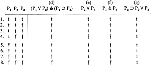
§4. Model theory: implication and equivalence. Suppose the truth table for a formula E is constructed as in § 2 by using exactly its prime components P₁ ..., P_n, and suppose that a new table is constructed for E using additional atoms P_n+1, . . . , P_n+m not in E. Then the new table differs from the original table only in that the value column of the new table splits into 2^m parts, corresponding to the 2^m assignments of ’s and ’s to the atoms P_n+1, . . . , P_n+m which do not occur in E. Each of these 2^m parts is a duplicate of the value column of the original table, since the same computation (based only on the assignments to P₁, . . . , P_n) is used in each part. For example with n = 2 and m = 1, Tables (e), (f), (g) below have been constructed by entering from three atoms, although the formula at the head of each of those tables contains just two atoms.

In Tables (e) and (g), Lines 5-8 (P₁ is ) are duplicates respectively of Lines 1-4 (P₁ is ); and in Table (f), Lines 3, 4, 7, 8 (P₂ is ) are duplicates respectively of Lines 1, 2, 5, 6 (P₂ is ).

In particular, if the table for a formula E entered from only its prime components contains only ’s, then so does the table for E entered using given additional atoms; and conversely. (This is illustrated by Table (g).) Thus, E if and only if the table for E entered from any particular list P₁, . . . , P_n (containing at least all the prime components of E) has only ’s.

In theorem 3 and 4, we shall compare truth tables for A and B (also for A⊃B or A B). To make this easy, we shall enter each table from one list of atoms P₁, . . . , P_n, including all that occur in either of A and B. So if A and B do not contain the same atoms, the table for A or for B is entered from more atoms than occur in it. By the preceding discussion, it will make no difference if the list P_l, . . . , P_n contains still more atoms.

THEOREM 3. If A and A⊃B, then B.

PROOF. Consider any assignment of ’s and ’s to a list P₁, . . . , P_n of atoms as described. The computation of the corresponding value of A⊃B consists in first computing the values of A and B, and thence computing the value of A⊃B by the table for ⊃ (beginning of § 2). By the hypotheses that A and A⊃B, both the value obtained for A and the final value for A⊃B are . From the table for ⊃, this can only be the case when Line 1 of that table applies, and in Line 1 of that table B is also t. Since this is the case for each assignment to P₁, . . . , P_n, the formula B receives the value t for all assignments, i.e. B, as was to be shown.

THEOREM 4. (a)For each assignment, is if and only if A and B have the same truth value. Hence: (b)° B if and only if A and B have the same truth table.

PROOF. Consider any formulas A and B. (a) In the computation of the value of for a given assignment of ’s and ’s to P₁, . . . , P_n the first part consists in computing values of A and B, after which the computation is concluded by entering the basic table for in § 2 with the resulting values of A and B. From that table we see that is if and only if the values computed for A and B are the same, (b) So the table for our has all ’s, exactly if, for every assignment, A and B have the same value.

EXAMPLE 2°. By (b) of the theorem with the result of Exercise 2.1 (a), (and ). Thence by substitution (Theorem 1), (and ). Thus we reprove *59 of Theorem 2. (This proof differs from the one suggested in § 3 only in that we now take into account the general principle stated as theorem 4 (b) ,instead of (like robots) separately completing the computation of in each line.

THEOREM 5. (Replacement theorem.) Let C_A be a formula containing a formula A as a specified (consecutive) part, and let C_B come from C_A by replacing that part by a formula B. If then .

PROOF. Assume . Then by theorem 4 (b) , A and B have the same table. Hence if, in the computation of a given line of the table for C_A, we replace the computation of the specified part A by a computation of B instead, the outcome will be unchanged. Thus C_B has the same table as C_A; so by theorem 4 (b),

EXAMPLE 3°. From Example 2 by theorem 5,

The part A of C_A is underlined. In writing C_B, a pair of parentheses is required which was unnecessary in C_A.

By a “consecutive” formula part A of C_A we are understanding a formula part A which is consecutive before parentheses are omitted, and whose value is thus computed in the course of computing the value of the whole C_A. Thus P ∨ Q does not occur as a consecutive part of , as becomes clear upon restoring some parentheses: .

COROLLARY. (Replacement rule, or replacement property of equivalence.) IfC_A and , then C_B

PROOF. By the hypothesis that with the theorem, . So by theorem 4 (b), C_A and C_B have the same table. By the hypothesis that C_A, this table has all ’s.

EXERCISES. 4.1. In the manner of Example 2, reprove *31, *34, *49, *55a, *55c of Theorem 2.

4.2°. Similarly establish that:

(a)

(b)

4.3. Illustrate the proof of theorem 5 by computing the second line (for assigned to P Q) of the tables for and . Underline the common parts (as in Table (a), (b)).

4.4°. Use theorem 5 with *55a in Theorem 2 to establish that .(Observe that, whatever formulas constructed from P, Q, R, . . . , P₁ P₂, P₃, . . . “A” and “B” stand for here, *55a will hold when its A and B are the present A and B.)

4.5. Using (Example 2), infer *10a from 5a.

4.6. Give three proofs that: If A and , then B.(By theorem 4 (b); by corollary theorem 5; using 10a and theorem 3.)

4.7. Show by an example that corollary theorem 5 does not hold with “⊃" in place of "”.

4.8. Establish the following propositions, where A is a formula containing no occurrence of the symbol , and B is any formula.

(a) The truth table of A has in its first line.

(b) If , then B contains at least one occurrence of .

§5. Model theory: chains of equivalences. It is often useful to know that two formulas A and B have the same truth table, or to transform a given formula A into a formula B of some specified sort which has the same table. By theorem 4 (b), A and B have the same table exactly when , i.e. when the formula asserting the (material) equivalence of A and B is valid. In this case, we may say that A and B are (logically) equivalent (in the propositional calculus). Of the 45 results in Theorem 2, 26 are thus assertions of equivalences holding in the propositional calculus.

The chain method which we present next is useful in establishing such equivalences.

First note that: if and only if both A and B. This is immediate from the truth table for & (or we can infer it by theorem 3 from 3, 4a and 4b in Theorem 2).

Next we observe that equivalence in the propositional calculus is reflexive, symmetric and transitive: . , then . (δ) If and , then . These three statements are immediate from theorem 4 (b). (Alternatively, (β) is *19; (γ) follows from *20 by Exercise 4.6; and (δ) from *21 using (α) and theorem 3.)

Using (β)-(γ): () if and and , then for each of the 16 pairs of subscripts i, j (i, j = 0, 1, 2, 3); i.e. . Thus (α) gives ; to get , we use and with (δ), and the result with (γ); etc. Or () can be recognized as true directly from theorem 4 (b); for, the three hypotheses of () say that in the list A₀, A₁ A₂, A₃ each successive formula has the same table as the preceding, and the conclusion says that any pair of formulas in the list have the same table.

Now we adopt as an abbreviation for . Then by two applications of (α): (). The hypothesis of () is equivalent to .

We call “chain of (three) equivalences”. It has the properties that we can establish its validity by establishing the validity of the (three) “links”, and that once the chain is established as valid we can infer the equivalence of any pair of the formulas A₀, A₁, A₂, A₃ (joined by links) in the chain.

Everything beginning with () said using A₀, A₁, A₂, A₃ applies similarly to A₀, . . . , A_n for any n ≥ 2 (and trivially even for n = 0, 1).

Now we remark that, once *49, *55a and *55c in Theorem 2 are established (as proposed in § 3, or by Exercise 4.1), then all of *55b, *56-*61 follow by the chain method. For example:

*55b. By *49 (since the A of *49 can be any formula, e.g. the present ) and (γ): (1) . By theorem 5 with *55a (as in Exercise 4.4):

(2) . By theorem 5 with *49:

(3) ,

(4) . From (l)-(4) by () (for n = 4),

, as was to be shown. — Using ( ), we can put this proof in the following shorthand:

Since in § 3 we could accept all the results of Theorem 2 as established by someone else’s computation, the real point of these reproofs is to make it evident how, if we remember *49, and any two of *55a-*61 which together contain all three of the symbols ⊃, &, ∨, we can quickly derive the others.

Now we use the chain method to get a new result.

THEOREM 6°. Let E be any formula constructed from atoms P₁, . . . , P_n and their negations using only & and ∨. Let come from E by interchanging & with ⊃ and each unnegated atom with its negation (cf. the example in the proof).¹⁹ Then .

PROOF. Using *55a and *55b (with the chain method), we can move the initial of progressively to the right (inward) across all the &’s and ∨’s, which interchanges them. Then we can use *49 to remove the resulting double negations, so that the atoms will be interchanged with their negations. The following example illustrates this proof.

COROLLARY°. Each formula E is equivalent to a formula F (i.e. ) in which occurs only applied directly to atoms.

PROOF. First, we can eliminate and ⊃ from E by *63a, and *58 or *59 (or possibly *55c, *60 or *61). Next, we can suppress any double negations by *49. Finally, theorem 6 can be used to eliminate successively each which does not apply directly to an atom; in doing so, we work each time on such a that is innermost (i.e. does not have another such within its scope, Example 1). This should become clear from the following illustration.

As we eliminate the ⊃, we supply a pair of parentheses, which before were superfluous since ⊃ outranks &. In the fourth and final formulas, we omit a pair of parentheses (as mathematicians do in writing “a+b+c”), since by *31 and *32 it is immaterial for present purposes which way the triple conjunction and disjunction are associated.²⁰

EXERCISES. 5.1. Use the chain method to derive *56, *58, *59, *61 (taking *49, *55a-*55c as already established).

5.2. Find equivalent formulas with applied only to atoms:

5.3°. Establish the following, using as far as possible recent results rather than new direct appeals to truth tables:

*§ 6. Model theory: duality.²¹ THEOREM 7°. (Duality.) Let E and F be formulas of the type described in Theorem 6. Let E′, F′ come from E, F by interchanging & with ∨.¹⁹ Then:

PROOF, (a) Assume . By Theorem 6 with corollary theorem 5 (or Exercise 4.6), . Thence by Theorem 1, * where * indicates the substitution of simultaneously for the atoms P₁, . . . , P_n. Finally, by *49 with corollary theorem 5, where indicates the removal of a double negation before each prime part which in E was unnegated. But is E′, as the following example illustrates.

(b) Assume . Then by *49 with colloary theorem 5, So by Theorem 6 and corollary theorem 5, . Thence . Thence , i.e. .

If we had established 4a, 4b, *31, *33, *35, *37, *39, *50 and duality (Theorem 7), but not yet 5a, 5b, *32, *34, *36, *38, *40, *51, the latter would follow by duality and substitution (Theorem 1). For example, by *50 with P as the A,. Thence by duality (Theorem 7 (a) ),. Thence by substitution, which is *51.

The effect of using Theorem 1 (substitution) with Theorem 7 is to allow the duality transformation to be applied to a resolution of E (or of E, F) into components A₁, . . . , A_n not necessarily prime, which must then retain their identity (be “treated as prime”) throughout the transformation. (Similarly with Theorem 6 and corollary.) —

Suppose a visitor from Mars is confused by what he observes upon his arrival on Earth, and mistakes our true “” for false “F”, and our false “” for true “T”; i.e. let F = and T = . Then our table for & would for him read as our table of ∨ for us, and vice versa. To see this, let us view the tables in the square arrangement (available in the case of two components), in which properties of the tables are more easily visualized. Table (1) is our table for &; (2) is the same rewritten using F = and T = ; (3) is (2) rearranged to the normal order of T first and F second (according to the Martian’s ideas). Now observe that Table (3) looks just like our table (4) ) for ∨, except that it is written in the capitals T, F instead of the small letters , . The table for written with T, F in the Martian’s normal order will look just like our table for written with , , as the reader may verify.

These observations suggest new proofs of Theorems 6 and 7.²² Also they suggest how to avoid excluding and ⊃ from the formulas E, F (and our restriction on was inessential above). We need simply add to our symbolism two new propositional connectives and , choosing the tables for and so that they will look to the Martian as the tables for and ⊃, respectively, look to us. The reader may verify that this is accomplished if has the table for and has the table for . We may, if we wish, regard these as temporary additions to our symbolism, used while applying duality, and then eliminated by rewriting each part by Exercise 5.3 (b)) and as .

We now prove Theorem 6a° (= Theorem 6 when E may be any formula, even containing and , and ^† is the operation of interchanging with , and ⊃ with , and & with V, and of changing by one the number of ’s on each atom). By theorem 4 (b) it will suffice to show that and E^† have the same table. In computing (any given line for) we first compute a value for E (from the ’s and ’s assigned to the atoms P₁, . . . P_n) using our tables for and then (by the of ) we change the resulting or to T or F. In computing E^† we first change the ’s and ’s assigned to P₁, . . . , P_n to T’s and F’s (by the change by one in the number of ’s on P₁, . . . . , P_n), and then (because of the interchange of with , and ⊃ with , and & with ∨) we do the same computation using the Martian’s tables with T, F as before we did using ours with , . Thus the two computations differ only in whether we change , to T, F at the end or at the beginning.

We prove Theorem 7a° (= Theorem 7 similarly extended), thus.

(a) {} ≡ {all lines in the table for have } ≡ {all lines in the table for ’ have T} ≡ {all lines in the table for ’ have } ≡ {all lines in the table for E′ have } ≡ ²³

EXERCISES. 6.1. Prove Theorem 7 (d) . (b) From the proof of Theorem 7a (a), infer (b). (c) Prove Theorem 7a (d) .

6.2. By applying Theorem 7a (c) (with P, Q, for A, B), extend the list in Example 5.3 (a) of “equivalents” of

§ 7. Model theory: valid consequence. We started this chapter by saying that logic has the important function of saying what follows from what, and thus of saying what propositions are theorems for given axioms. Yet thus far we have dealt only with tautologies, i.e. valid formulas, which logic asserts to hold without regard to any extra-logical assumptions whatsoever.

Still keeping in mind that in the propositional calculus we do not look at the internal structure of the atoms (or will not know the propositions they express), let us suppose that we are given from outside the propositional calculus that a formula A is true by assumption or fact. That is, we may be told that it is an axiom of some abstract theory (like geometry or group theory), so it is true by fiat for the purpose of that theory. Or it may be a proposition which is true in physical fact or by intuitive mathematical reasoning. How does this alter our position with regard to what formulas we can assert to be true by use otherwise of only the propositional calculus?

Consider an example; say A is (P ⊃ Q) & (P ∨ R) (Table (h)).

Remember that what P, Q and R really are is top-secret information, and practitioners of the propositional calculus are not cleared for it. Nevertheless, if we are told that (P ⊃ Q) & (P ∨ R) is true, we have been told something. Namely, we then know that the truth values of P, Q, R must form one of the four assignments (Lines 1, 2, 5, 7) which give t to (P ⊃ Q) & (P ∨ R) in Table (h). So now, in trying to decide what other formulas B are true on the basis of the propositional calculus plus the information that A is true, we need consider only these four assignments. Thus, upon being given that A is true, we know that Q V R is true because its table (i) has only ’s in Lines 1, 2, 5, 7; but we still do not have enough information to know whether P ⊃ Q is true, because its table (j) has in Line 2.

This leads us to the following definition. Consider two formulas A and B, and let P₁, . . . , P_n be the atoms occurring in A or in B. We say that B is a valid consequence of A (in, or by, the propositional calculus), or in symbols , if, in truth tables for A and B entered from P₁, . . . , P_n, the formula B has the value in all those lines in which A has .

Thus, as we have just observed, but not .

We note that “” is a stronger statement than “If , then ”; by this we mean that the first statement always implies the second, but the second may hold without the first holding.

To see that the first always implies the second, assume the first “” and the hypothesis “” of the second. Then (by ) B has in all those lines in which A has ; and (by ) these are all lines; so .

When A, B are (P ⊃ Q) & (P ∨ R), P ⊃ R, the second statement “If , then ” holds as a material implication (§ 2) since “” is false; but as we observed above “” does not hold. The point is that, when not , so it is not the case that A is in all lines, then “If , then ” holds automatically, while “” holds only if B is in those lines if any in which A is .

Now suppose m formulas A_l, . . . , A_m are given. Generalizing from the case m = 1, we define: B is a valid consequence of A₁, . . . A_m (in, or by, the propositional calculus), or in symbols , if, in truth tables entered from a list P₁, . . . , P_n of the atoms occurring in one or more of A₁, . . . , A_m, B, the formula B is in all those lines in which A₁, . . . , A_m are simultaneously . The symbol may be read “entail(s)”.

Not only is it obviously immaterial here in what order the atoms occurring in any of A₁, . . . , A_m, B are listed as P₁, . . . , P_n. But also by beginning § 4, the outcome will be the same if the tables for A₁, . . . A_m, B are entered from a list P₁, . . . , P_n including still more atoms.

Inspection of the tables shows that (Lines 1, 3, 5, 6, 7); (Line 3); (there are no lines in which it needs to be checked that (i) is ); but not (h) (e.g. Line 3).

THEOREM 8. (a) if and only if (b) More generally, for if and only if .

PROOF, (a) Consider tables for A, B, A ⊃ B entered from a list P₁, . . . , P_n including all their atoms. Those lines in which A is do not matter for whether , and in those lines A ⊃ B is anyway (by the table for ⊃). So consider the remaining lines, i.e. the lines in which A is . If , then B is in these lines; so by the table for ⊃, A ⊃ B is in these lines (as well as the others); so . Conversely, if , then A ⊃ B is in these lines (as well as the others); so by the table for ⊃, B is in these lines (the lines for which A is ); so .

(b) FOR m ≥ 2. Consider tables for A₁, . . . , A_m, B, A ⊃ B. We reason as before, with A_m as the A, except that we confine our attention throughout to only lines in which A₁, . . . , A_m-1 are .

COROLLARY. For if and only if

PROOF. By m successive applications of the theorem.

By corollary Theorem 8, the problem of what formulas are valid consequences of given formulas A₁, . . . , A_m is reduced to the problem of what formulas are valid. This is one reason why tautologies are important.

One might reverse the argument and consider this as a reason why the valid consequence relationship is unimportant. However, the valid consequence relationship corresponds more directly to the way we ordinarily use logic. Many manipulations are easier to make in terms of valid consequence relationships than when these relationships are condensed by corollary Theorem 8 into the validity of iterated implications.

For reasons which will appear later, we prefer to emphasize these manipulations in another context, that of “proof theory”, which we will begin studying in § 9. Therefore we relegate the further development in terms of valid consequence to the exercises, which may help to make some of the manipulations more meaningful when we take them up in proof theory.

EXERCISES. 7.1. (a) Find all the true statements “” and “” where B is one of . (Counting trivial ones like “”, there are six.) (b) Prove that for every formula . (c) Prove that for every formula if and only if .

7.2. Verify by truth tables: (a) . (b) . (c) . (d) . (e) (f) not .

7.3. Show that, with notation as in Theorem 1 (but with m + 1 formulas): If , then . (HINT: use corollary Theorem 8.)

7.4. (a) Apply Exercise 7.3 to generalize Exercise 7.2 (a)-(e) from P, Q to A, B. (b) Thence by Theorem 8 and corollary reprove 3, 4a, 4b and *10a of Theorem 2.

7.5. For m ≥ 1, show that: (a) if and only if .²⁰ Thence by Theorem 8: (b) if and only if . (This gives us an alternative to corollary Theorem 8.)

7.6. Establish the following.

7.7. Show directly from the definition of valid consequence:

(a) If and , then . (Reductio ad absurdum.)

(b) If and then . (Proof by cases.)

7.8. Do Exercise 7.7 instead from Theorems 2, 8 and 3.

7.9. Observe that the reasoning in §§ 4, 5 (for the chain method) holds good when we confine our attention to assignments (i.e. lines of the tables) for which a given list of formulas A₁, . . . , A_m are all t; so Theorem 3, Theorem 5 (and corollary), and , and thus the chain method, hold good with “” replaced throughout by “”. Now show that:

(a) . (HINT: cf. Theorem 2.)

(b) .

*§ 8. Model theory: condensed truth tables. We used the idea of the truth tables to define when a formula E is valid (in symbols, E) and when a formula B is a valid consequence of formulas A₁, . . . , A_m (in symbols, ). The tables themselves have been used (often with shortcuts, as in Exercise 2.3) in illustrations and in the original proofs of the results in Theorem 2 and some other results. But hereafter, to establish that E or that , it will ordinarily be more efficient to employ theorems about validity and “valid consequence” than actually to compute truth tables. In §§ 4 and 5 we began, and we shall continue, to develop techniques for using such results systematically in lieu of truth tables. If we wish to show that not E or not , we need to compute only one suitably chosen line of the table(s). Often we can spot such a line with a little trial and error, without computing the full table(s).

A formula E is called inconsistent or contradictory or identically false, if it has a solid column of ’s in its truth table; contingent, if it is neither valid nor inconsistent. Thus formulas fall into three classes with respect to the presence of ’s and ’s in their truth tables.

A formula E is inconsistent or consistent, according as is valid or invalid. To establish that a formula is contingent, computation of two suitable lines would suffice.

If, notwithstanding, we should find we need to do much truth-table computation, it will be worthwhile to seek further economies in the writing and computing of the tables.²⁴ We used 8 lines in writing the tables for formulas with 3 atoms; with a dozen atoms, 4096 lines would be required similarly.

Consider the table (1) in § 2 for . Since the value is common to the last four lines, those lines can be replaced by one. Likewise, the first and third, and also the second and fourth, lines can be combined. Thus (1) condenses to:

In § 2, we observed a shortcut in the computation of the table for which gave the ’s in the last four lines of (1) en masse. This shortcut is an instance of a technique that is advantageous generally. The technique consists in assigning a value or to just one of the letters and computing as far as we can with that, then repeating with another letter, etc. (instead of assigning values to all of the letters first, and computing second). Consider the basic table for any binary proposi-tional connective O. If we pick a value ( or ) for A, then, with that value fixed, A O B has the table of a unary connective applied to B. There are only four possible tables for a unary connective, with entries respectively : (i) , , (ii) , (the same as the values of B), (iii) , (the same as ), (iv) , . So, after picking a value of A; A O B can be evaluated as one of , B, , . Considering the actual cases that interest us, we obtain the following tables.

Now we use this technique on the previous example.

In the first line is the formula before values have been assigned to any of the letters. In the second line, P has been assigned and in the left and right columns, respectively. The tables in (I) are then used to simplify the resulting expressions to iR in the left column (by three steps) and to in the right column (by one step). Continuing, in the fourth line of the left column, R is assigned and in the left and right subcolumns, respectively. The figure (3) is called a truth-value analysis by Quine 1950, who was apparently the first to emphasize the advantages of computing on one letter at a time. The table (2) can be read off the analysis (3) (and indeed Quine in 1950 never writes (2) at all).²⁵

A good rule of thumb is to select each time, for assignment of or , a letter occurring frequently. This will tend to promote rapid simplification, as each binary combination in which it occurs must disappear. By looking ahead a bit, one may be able to recognize cases when a different choice would be better.

Steps can be saved by using *49 (with Theorems 4, 5) to suppress double negations, either present initially or introduced in using (I). Thus if B is simplifies by (I) to , which further simplifies by *49 toC.

The method of (3) is not guaranteed to bring us directly to a most condensed table, like (2). If we treat Q second (instead of R), we come out with a 5-line table.

The formula admits the table (2); but no order of treating the letters gives a 3-line table directly. Of course, afterwards we can combine lines, as we did to get (2) from (1). If we first notice that ((Q ⊃ P) ⊃ Q) ⊃ Q is valid (Exercise 2.3 (a)), we can pass to , and thence to (2).

Indeed, the method of (3) will never produce a table of less than two lines, since it requires an assignment of or to one of the letters P₁ to get started. But ((Q ⊃ P) ⊃ Q) ⊃ Q, being valid, admits the 1-line table:

Full truth tables, preferably written in condensed form, can be used in simplifying formulas. Suppose a complicated formula E arises in some problem, and we wish to investigate valid consequences of E, or more generally to investigate whether various relationships hold in which E is a specified one (or a part of one) of A₁, . . . , A_m, B. For these purposes, E can be replaced by any formula F with the same truth table as E (i.e. by Theorem 4, a formula F such that ), or as we said in § 5 a formula F equivalent to E (in thepropositional calculus). So if we can find a formula F equivalent to E but simpler than E, our investigation will be furthered.

For example, say E is or , either of which has the truth table (2). By starting from (2), and asking what formulas have that truth table, we find ones simpler than E, namely (which is picked to have exactly the two ’s in (2)), (where P & R is picked to have exactly the one f in (2)), (thence by De Morgan’s law *55b), and (thence by *59). The formula gives a resolution of the truth of E into two disjoint (i.e. non-overlapping) cases (namely: P, R are , ; P is ), and condenses this by allowing the cases to overlap. Thus we could have found without going through .

It is worth noting that consolidation and recombination of cases can be effected by chains of equivalences, since facility with such transformations is useful. Besides results in Theorem 2, we need the following.²⁰

*52°. .

*53. .

*54. .

*55°. .

We give an illustration, starting with an equivalent of read from (1) with only the last four lines combined:²⁶

[*35 with *33 (and *31)]

[*52] [*36, *34]

[*52, *33].

Say that for any formula E we have found a p+q-line truth table (condensed or not) with p ’s and q ’s. As illustrated, we can then write an equivalent formula D of the form D₁ ∨. . . ∨ D_p (which reduces to simply D₁ if p = 1, and say to if p = 0) where D₁, . . . , D_P correspond to the respective ’s, and an equivalent formula C of the form C₁ & . . . & C_q (which reduces to C₁ if q = 1, and say to if q = 0) where C₁, . . . , C_q correspond to the respective ’s. To give another example, if E is , then D is and C is [by Theorem 6 from ]. Such a formula D (a disjunction of conjunctions of negated and unnegated atoms) equivalent to E is called a disjunctive normal form of E, and such a formula C (vice versa) a conjunctive normal form.

By a formula F being “simpler” than E we mean in a pragmatic sense that it is easier to comprehend and use, even if it is not shorter or much shorter. What is simpler will then depend on what uses we have in view, or on what sorts of formulas we have become adept at handling. (Thus we scarcely need to simplify .) Disjunctive normal forms of E are useful if we ,are endeavoring to infer valid consequences from E (cf. Exercise 7.7 (b)) or from E and other formulas, and conjunctive normal forms of E if we are endeavoring to infer E as a valid consequence of other formulas (cf. Exercise 7.2 (b)).

EXERCISES. 8.1. Establish *52-*55 with P, Q (preparatory to substituting A, B by Theorem 1) by using (I) with *50, *51 (and Theorem 4).

8.2. Simplify:

(a) .

(b) (Write a simple equivalent after treating only R and Q.)

§ 9. Proof theory: provability and deducibility. The proof of theorems, or the deduction of consequences of assumptions, in mathematics typically proceeds à la Euclid, by putting sentences in a list called a “proof” or “deduction”. We use the word “proof” (and call the assumptions “axioms”) when the assumptions have a permanent status for a theory under consideration, “deduction” when we are not thinking of them as permanent. Each step from some sentences in the list to another is mediated by logic, as analyzed above for the case the logic is propositional logic. Thus one sentence follows from others if it is a valid consequence of those others; this relationship we defined by truth tables in § 7. A sentence can be put into the list without reference to earlier sentences, if it is one of the assumptions or is valid. In the definitions of “valid consequence” and validity, we stood outside the language of the sentences themselves (the object language), and observed in another language (the observer’s language) how the sentences (or formulas) are composed from atoms. In the observer’s language, we also developed various results concerning validity and the valid consequence relationship which often are more convenient to use than direct application of the truth tables. We call this treatment of logic “model theory”, as in it we replace the atoms by truth values and f in all possible combinations, to obtain what can be considered models or concrete replicas of what the sentences may express.

Now we shall take up another way of founding logic. This treatment, called “proof theory”, arises from asking the question whether the proofs and deductions of logic itself cannot be given in an analogous way. But now, since it is logic itself that we would treat in the axiomatic-deductive manner, the inferences cannot be made by appealing to logical criteria but only to specifically stated axioms and rules. In proof theory, some sentences or formulas will be taken as logical “axioms”, and some “rules of inference” will be established for making the inferences from some sentences to another sentence.

We now give such a formulation of the classical propositional calculus, both by itself and for its application to deduction from assumptions. Later we shall show that the two formulations, that of model theory and that of proof theory, give equivalent results.

As axioms for our (proof-theoretic) system of the (classical) propositional calculus, we take all formulas of any of the forms shown after the symbol “” in la-10b of Theorem 2 (and in the “List of Postulates” p. 387). These forms themselves we call axiom schemata. Each axiom schema includes infinitely many axioms, one for each choice of the formulas denoted by “A”, “B”, “C”. For example, corresponding to la in Theorem 2, we have as Axiom Schema la: A ⊃ (B ⊃ A). Particular axioms by this schema are: P⊃(P⊃P),P⊃(Q⊃P),Q⊃(P⊃ Q), , , etc.

As the sole rule of inference, called the ⊃-rule or modus ponens or the rule of detachment, we take the operation of passing from two formulas of the respective forms A and A ⊃ B to the formula B, for any choice of formulas A and B (cf. Theorem 3). In an inference by this rule, the formulas A and A ⊃ B are the premises, and B is the conclusion.

We define a (formal) proof (in the propositional calculus) to be a finite list of (occurrences of) formulas B₁, . . . , B_l each of which either is an axiom of the propositional calculus or comes by the ⊃-rule from a pair of formulas preceding it in the list. A proof is said to be a proof of its last formula B^l. If a proof of a given formula B exists, we say B is (formally) provable, or is a (formal) theorem, or in symbols .

EXAMPLE 4. For each formula A, the following list of five formulas B₁, . . . , B_l is a proof of the formula A⊃A. (Here l = 5, and B₁ is A ⊃ (A ⊃ A), . . . , B₅ is A ⊃ A.)²⁷

1. A ⊃ (A ⊃ A) — Axiom Schema la.

2. {A ⊃ (A ⊃ A)} ⊃ {[A ⊃ ((A ⊃A)⊃ A)] ⊃ [A ⊃ A]} — Ax. Sch. lb.

3. [A ⊃ ((A ⊃ A) ⊃ A)] ⊃ [A ⊃ A] — modus ponens, 1, 2.

4. A ⊃ ((A ⊃ A) ⊃ A) — Axiom Schema la.

5. A⊃A — modus ponens, 4, 3.

Besides the proof itself B₁, . . . , B_l, we give at the left numbers for reference, and at the right reasons which justify the inclusion of each of the formulas B₁, . . . , B_l in the proof (an “analysis” of the proof). Thus at Step 1, we have applied Axiom Schema la with A both as the A and as the B of the schema (i.e. with the formula presently denoted by “A” as the formula denoted by “A” and by “B” in the statement of the schema). In Step 2, A is the A, A ⊃ A is the B, and A is the C, of Axiom Schema lb. In applying modus ponens to Formulas 1 and 2 at Step 3, the A of the rule is A ⊃ (A ⊃ A) (which is 1) and the B of the rule is 3. — Because 1-5 constitutes a proof (for any fixed formula A), we can say that A ⊃ A is provable, or in symbols . Similarly, , etc. (Why?)

A few remarks may help to make this way of formulating the propositional calculus as an axiomatic-deductive theory seem reasonable. We have an infinite number of axioms from each axiom schema, as mentioned above. This could be avoided by requiring the language in which the prime formulas are constructed to include single letters as “proposition variables” and adding a second rule of inference, the “substitution rule”, to say that E* can be inferred from E under the circumstances of Theorem 1 when P₁, . . . , P_n are proposition variables. That procedure seems less in keeping with usual mathematical language than the one we have followed (due to von Neumann 1927).²⁸

The list of thirteen axiom schemata may seem surprisingly long. However, each propositional connective must have axioms to characterize it, i.e. to provide the deductive properties we want it to have. We are getting along with only two or three axiom schemata for each of ⊃, &, ∨, , , namely, one or two (left column in Theorem 2) which help us to prove formulas in which the symbol is used (i.e. to “introduce” the symbol), and (except for ⊃) one or two (right column) which help us to infer formulas not containing the symbol (or not containing it so often) from formulas containing it (i.e. to “eliminate” the symbol). In the case of 3, the ⊃-rule provides for “elimination”. This (to our mind) elegant arrangement of axiom schemata is due essentially to Gentzen 1934-5.

We could get along with fewer axiom schemata by foregoing the use of some of the symbols &, ∨, as an official part of the object language. For example, if each time we wrote “A B” we understood it as an abbreviation for (A ⊃ B) & (B ⊃ A), then Axiom Schemata 9a, 10a, 10b could be omitted.²⁹

For the propositional calculus applied to infer formulas from assumptions A₁, . . . , A_m, the formulas A₁, . . . , A_m are in effect allowed to function as axioms also. However, we shall not call them “axioms” (for the propositional calculus), but (when we need a name) assumption formulas; and (for m > 0) we shall not call B₁, . . . , B_l a “proof”, but a “deduction” from A₁, . . . , A_m. That is, a finite list of (occurrences of) formulas B₁, . . . , B_l is a (formal) deduction (of B_l) from A₁, . . . , A_m (in, or by, the propositional calculus), if each formula in the list is one of A₁, . . . , A_m, or one of the axioms (of the propositional calculus, i.e. by one of Axiom Schemata la-lOb), or comes from two earlier formulas in the list by the ⊃-rule. If there is a deduction of a given formula B from A_1?. . ., A_TO, we say that B is deducible from A₁, . . . , A_m, or in symbols . The symbol “” may be read “yield(s)”. (In using this terminology when m≥.0, “deduction” and “deducible” include “proof” and “provable” as the case m = 0.)³⁰

EXAMPLE 5. For each choice of formulas A, B, C, the following sequence of 8 formulas is a deduction of C from A ⊃ (B ⊃ C), A & B.

1. A & B – 2nd assumption formula.

2. A & B ⊃ A – Axiom Schema 4a.

3. A – modus ponens, 1, 2.

4. A⊃(B⊃C) – 1st assumption formula.

5. B⊃C – modus ponens, 3, 4.

6. A&B⊃B – Axiom Schema 4b.

7. B – modus ponens, 1,6.

8. C – modus ponens, 7, 5.

Thus we can say that C is deducible from A ⊃ (B ⊃ C), A & B; or briefly, A ⊃ (B ⊃ C), .

We said “formal proof” and “formal deduction” in the definitions above (though we shall usually omit the word “formal”) to emphasize that these proofs and deductions are in the object language, which we are studying in the observer’s language (§ 1). From the standpoint of the observer’s language, we look only at the form of the formulas (in contrast to their meaning or content) in determining under the definitions just given whether a given sequence of formulas B₁, . . . , B_l is in fact a (formal) proof, or a (formal) deduction from given assumption formulas A₁, . . . , A_m. A sequence of formulas B₁, . . . , B_l, is a (formal) proof, or a (formal) deduction from B, only when it exactly fits the above definition (as illustrated in Examples 4 and 5.)³¹ This stereotyping of the operations that can be performed in constructing a formal proof or deduction makes the formal proofs and deductions (in the object language) definite enough in structure to serve as objects of our study.

In our study (in the observer’s language), we shall also be proving theorems, deducing consequences of assumptions, etc. This will be as much the case here in proof theory as it was in model theory. In these informal proofs and deductions, we may operate flexibly, on the basis of the meanings of our statements, using any inferences that carry conviction. (It may indeed be that some of these inferences are the informal counterparts of operations.available in the formal proofs, but they are not restricted to be such.)³²

The student who keeps in mind that there are the two languages, where now (formal) proofs and deductions as well as formulas in the one language (the object language) are being studied, using (of necessity) informal proofs and deductions in another language (the observer’s language), should have no trouble keeping matters straight. In model theory, the object language was dealt with only as an assemblage of formulas, whose truth tables we investigated; so there was not quite as much of a parallelism of terminology as we shall now have.

We conclude this section by giving in the observer’s language two easy (informal) theorems (and their proofs), which have as their subject or object formal proofs and deductions in the object language.

THEOREM 9.

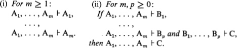
PROOF. (i) The definition of a deduction B₁, . . . , B_l does not require that each of the assumption formulas A₁, . . . , A_m actually occur in the list B₁, . . . , B_l. So, for each i from 1 to m,A_i standing by itself constitutes a deduction of C from A₁, . . . , A_m. (ii) In a given deduction of C from B₁, . . . , B_l we can replace the occurrences of the assumption formulas B₁, . . . , B_l by deductions of B₁, . . . , B_l respectively from A_l9 . . ., A_m. Thereby we obtain a deduction of C from A₁, . . . , A_m. —

Let A₁, . . . , A_m be a given list of formulas. Suppose we are exploring the class of the formulas B which are deducible from A₁, . . . , A_m. Theorem 9 (i) tells us that A₁, . . . , A_m themselves are in this class. Theorem 9 (ii) tells us that any formula C is in this class which is deducible from any formulas B₁, . . . , B_l already known to be in this class.

From this standpoint, the role of Theorem 9 should be clear. However, we shall return to this in § 13, after obtaining some practice meanwhile with particular applications of Theorem 9 . —

Before continuing, it may be well to contrast the meanings of four expressions.

“” means that the formula A ⊃ B is valid, i.e. its truth table has a solid column of t’s.

“” means that the formula B is a valid consequence of the formula A, i.e. B has t in each of those lines of its truth table in which A has t.

“” means that the formula A ⊃ B is provable, i.e. there is a finite sequence of formulas such that each formula of the sequence either is an axiom or comes from two preceding formulas of the sequence by modus ponens, and the last formula of the sequence is A ⊃ B.

“” means that the formula B is deducible from the formula A, i.e. there is a finite sequence of formulas such that each formula of the sequence either is A or is an axiom or comes from two preceding formulas of the sequence by modus ponens, and the last formula of the sequence is B.

By the end of § 12, we shall have found that these four expressions are equivalent, i.e. if any one is true so are the other three. (For the first two, we have this already in Theorem 8.)

Likewise, we shall find that “If , then ” and “If , then ” are equivalent. These two expressions are weaker than the preceding four, as we have already seen in § 7 for the ones with “”

THEOREM 10. (a) If , then . (b) More generally, for any m≥1: If , then .

PROOF. (b) By hypothesis, there is a deduction of A_m ⊃ B from A₁, . . . , A_m-1 (say it has k formulas). Using this, we can construct a deduction of B from A₁, . . . , A_m-1, A_m as follows.

k+1. A_m — mth assumption formula.

k+2. B — modus ponens, k+1, k.

COROLLARY. If , then .

EXERCISES. 9.1. Add to 1-5 in Example 4 to make a proof of A A.

9.2. The following is a deduction of C from A, B, A ⊃ (B ⊃ C). Supply the reasons (or “analysis”), and state the result using “ ”.

1. A.

2. A ⊃ (B ⊃ C).

3. B ⊃ C.

4. B.

5. C.

9.3. By constructing appropriate deductions, show that:

9.4. Supply missing hypotheses (and justify them) or conclusion in the following applications of Theorem 9 (ii) :

(a) and ; therefore—– (m = 2, p = 1.)

(b) —– and ; therefore A ⊃ (B ⊃ C), . (m = 2, p = 1)

(d) —– and —– and A, ; therefore A, , . (m = 3, p = 2).

9.5. Corresponding to Exercise 9.4 (c), illustrate the proof of Theorem 9 (ii) by combining the deductions of Exercise 9.3 (c) and (d) (construed as deductions from A ⊃ (B ⊃ C), A & B) with that of Exercise 9.2. Compare your result with Example 5.

9.6. Write out the m = 0 and p = = 0 cases of Theorem 9 (ii) and adapt the proof to them.

9.7. Show how the result of Exercise 9.1 (i.e. ) comes by Theorem 9 from . (Example 4) and Exercise 9.3 (h). (Take m = 0.)

9.8. Show that: If , then .²⁰

§ 10. Proof theory: the deduction theorem. The property of deducibility expressed by the next theorem corresponds to a familiar method in our informal reasoning. To establish an implication “If A, then B”, we often assume A “for the sake of the argument” and undertake to deduce B. This method is also available in the presence of other assumptions A₁. . ., A_m-₁.

The proof is longer than that of the preceding theorems (except Theorem 2, if all the computations are included). But it has a simple plan, after which the rest of the work falls into four simple cases.

THEOREM 11. (The deduction theorem, Herbrand 1930.)³³ (a) If , then . (b) If , then .

PROOF. (b) The student should first review exactly what the hypothesis and conclusion mean under our definition of “ ”. (Each asserts the existence of a certain kind of a finite list of formulas, say B₁, . . . , B_l and B′₁, . . . , B′_p. There are two differences in the specifications for these two lists. In the first list but not in the second, a formula may be inserted on the ground that it is the mth assumption formula A_m. In the first list the last formula must be B, in the second A_m ⊃ B.)

We must show that, whenever we are given a deduction of B from A₁, . . . , A_m-1, A_m (the “given deduction”), we can find a deduction of A_m ⊃ B from A₁, . . . , A_m-1. There is in fact a uniform method by which, from any such given deduction, we can always find a deduction of A_m ⊃ B from A₁ from A₁, . . . , A_m-1 (the “resulting deduction”). We describe this method in general terms now, and in Example 6 below we illustrate it.

Say the given deduction is

so B_t is B. (In Example 6, (α) is the left column, consisting of Formulas 1-5.) As the first step toward constructing the resulting deduction, we prefix to each formula of the given deduction (α) the symbols A_w ⊃, supplying parentheses as appropriate. Thus we obtain

which does have last the formula A_m ⊃ B which must be last in the resulting deduction. (In Example 6, (β) is 3′, 8′, 11′, 14′, 17′ in the right column.) But this sequence (β) is not in general a deduction from A₁ from A₁, . . . , A_m-1. However we can insert some additional formulas into it before each one A_m ⊃ B, of its formulas (i = 1, . . . , l) so that it will become a deduction (y) from A₁ from A₁, . . . , A_m-1. For each i, the choice of the formulas to be inserted before A_m ⊃ B, depends on the reason given for the inclusion of B^ in the given deduction (α).³⁴

CASE 1: B_i is one of the first m-1 assumption formulas A₁ from A₁, . . . , A_m-1, which are retained as assumption formulas for the resulting deduction; say B_i is A_j (j < m). Then we insert the first two of the following formulas before the third, which is A_m ⊃ B,.

k′.	A_j — jth assumption formula.
k+1′.	A_j ⊃ (A_m ⊃ A_j) — Axiom Schema la.
k+2′.	A_j ⊃ A_j — modus ponens, k′, k+1′.

(In Example 6, this is illustrated by l′-3′ with k′ = 1′, and again by 9-11′ with k′ = 9′.)

CASE 2: B_l is the last assumption formula A_m, which will not be retained as an assumption formula for the resulting deduction (unless A_m happens to be the same formula as one of A₁, . . . , A_m-1). We insert the first four of the formulas in the proof of A ⊃ A in Example 4 for A_m as the A. (In Example 6, this is illustrated by 4′-8′, A_m being A so the insertions read exactly as in Example 4.)

CASE 3: B_l is an axiom. Treated similarly to Case 1. (Not illustrated in Example 6.)

CASE 4: B_l comes from two preceding formulas B_g and B_h (g, h < i) by modus ponens. We leave it to the reader as an exercise to work out the treatment of this case, and to supply the insertions 12′, 13′ and 15′, 16′ in Example 6 (Exercise 10.1).

EXAMPLE 6. To illustrate the proof of the deduction theorem, we give: (α) in the left column, a deduction of C from A⊃(B⊃C), B, A; and (γ) in the right column, the deduction of A⊃C from A⊃(B⊃C), B resulting from that given deduction by the uniform method described in the proof of the theorem.

(A simplification applicable to this particular example leads to a shorter deduction of A ⊃ C from A⊃(B⊃ C), B. Indeed, the 7 formulas 1′, 2′, 3′, 9′, 15′, 16′, 17′ suffice in place of the 17 which our uniform method gives.)

Applying the uniform method to l′-17′ as the given deduction leads to a deduction l″-53″ of B⊃(A⊃C) from A⊃(B⊃C); and application of the method to this in turn leads to a proof 1—161 of (A⊃(B⊃ C)) ⊃(B⊃(A⊃ C)). (Cf. Exercise 10.2.)

We wrote out the 17-formula deduction of A ⊃ C from A⊃(B⊃ C), B resulting by our method applied to 1-5 in order to help the reader visualize the proof of the deduction theorem. But now that the deduction theorem is proved, we shall be satisfied to use it to infer the existence of deductions and proofs without actually constructing them. Thus actual construction of the deduction 1-5 (left column) establishes that . Thence it follows by three successive applications of Theorem 11 that , and finally that, i.e. that there exists a proof of the formula (A⊃(B⊃ C)) ⊃(B⊃(A⊃ C). This satisfies us; we have no interest in actually seeing a proof of that formula, least of all the 161-formula proof resulting by three successive applications of our uniform method to the 5-formula deduction in the left column of Example 6. (There are shorter proofs of (A⊃(B⊃ C)) ⊃ (B ⊃ (A ⊃ C)). Using the simplification of l′-17′ noted above before reapplying the uniform method, we get one having 71 formulas.) But while our uniform method in the proof of Theorem 11 may be uneconomical for constructing deductions and proofs, it is efficient for proving Theorem 11; and Theorem 11 itself is very efficient for establishing their existence. We believe the reader right after Example 5 would have found it a fairly difficult exercise to construct (or show the existence of) a proof of (A ⊃ (B ⊃ C)) ⊃ (B ⊃ (A ⊃ C)).

Changing the letters in the preceding illustration (which we can do since A, B, C were arbitrary formulas, e.g. the B, A, C of the next), . Now using Axiom Schema 9a and modus ponens twice, (cf. *3).

COROLLARY. If , then .

EXERCISES. 10.1. Treat Case 4, and supply 12′, 13′, 15′, 16′ in the right column of Example 6.

10.2. Show that, when the given deduction has l formulas, the resulting deduction has 3l + 2 formulas if A_m is used as such in it; otherwise, 3l formulas.

10.3. Show that (start by constructing an appropriate deduction) and (using Example 7) (cf. *4a).

10.4. Show that (cf. *2).

10.5. Show that: If , then .

§ 11. Proof theory: consistency, introduction and elimination rules. The corollaries to Theorems 10 and 11 accomplish the reduction of the deducibility notion “” to the provability notion “” in a manner parallel to the reduction of the notion of valid consequence “” to the notion of validity “” given in corollary Theorem 8.

Hence, if we can show that “ ” and “” are equivalent, we shall then have completed the demonstration of the equivalence of proof theory and model theory for the propositional calculus, both as used in treating absolute logical truths and when applied under assumptions A₁ . . ., A_m. We do this in Theorems 12 and 14.

THEOREM 12. Each provable formula E is valid; using our symbols: if , then .

PROOF. By 1a-10b in Theorem 2, each axiom of the propositional calculus is valid. By Theorem 3, given that the premises A and B for an application of modus ponens are valid, so is the conclusion B. Thus, as we construct a proof B₁, . . . , B_l of E, each of the formulas B₁, B₂, B₃, . . . successively introduced (either as an axiom, or as a consequence by modus ponens) is valid. Therefore, the last formula B_l, which is E, is valid.

COROLLARY. For no formula B are both B and provable; using our symbols: for no formula B do both and hold.

PROOF. Suppose and for some B. Then by the theorem, and ; i.e. B has all t’s in its truth table and so does . This is absurd, since, by the table for , if B has all t’s then has all ’s. —

In general, by a “consistency property” of an axiomatic-deductive system (to be called a “formal system” in § 37) we mean a property that at most certain formulas are provable (e.g. only ones having some desired property, or lacking some undesired property). By a “completeness property”, we mean a property that at least certain formulas are provable (e.g. all having a certain desired property).

Thus Theorem 12 establishes “consistency of the propositional calculus with respect to validity”, and its corollary establishes the so-called “simple consistency”.

To establish the converse of Theorem 12 (Theorem 14, giving the “completeness of the propositional calculus with respect to validity”). we shall need to develop the proof theory of the propositional calculus for a certain distance. In this development, the deduction theorem (Theorem 11) is a most helpful tool. We begin (in Theorem 13) with a collection of fourteen rules adapted from Gentzen 1934-5, which we call “introductions” and “eliminations” of logical symbols. For completeness, we include the deduction theorem itself as “⊃-introduction”, and modus ponens restated using “ ” as “⊃-elimination”. The rest of the rules (with one exception, “weak -elimination”) amount essentially to restatements of the axiom schemata in the light of these two rules. To save space, we let “Γ” stand for a list of zero or more formulas, so we can write “” for “” with A_m = A(Γ empty for m = 1).

The rule of -introduction (next to the bottom in the left column) corresponds to the informal method of “reductio ad absurdum”: to prove “not A” or that A is false, we assume A “for the sake of the argument" and deduce a contradiction B and “not B”. This argument can be carried out in the presence of prior assumptions Γ

The rule of V-elimination corresponds to the informal method of “proof by cases”. If we have established “A or B” or are assuming this, then to show that C follows it suffices to show it in two cases, the case that A holds and the case that B holds. (For the problem of deducing C from A ∨ B, we can thus “eliminate” the ∨, and attempt the deduction from A and from B separately. It is in this sense that we can consider the rule as an elimination rule.)

THEOREM 13. For any finite list of (zero or more) formulas Γ, and any formulas A, B, C:

PROOFS. We already have ⊃-introduction in Theorem 11, and D-elim., &-introd., &-elim., V-introd., (double) -elim. and the three -rules in Exercise 9.3.

V-elimination (proof by cases).

1. — hypothesis.

2. — hypothesis.

3. ⊃-introd. (the deduction theorem), 1.

4. ⊃-introd. (the deduction theorem), 2.

5. using Axiom Schema 6, and modus ponens thrice. (That is, we can construct the following deduction:

1′. A⊃C. 2′. (A ⊃ C) ⊃ ((B ⊃ C) ⊃ (A ⊃ B ⊃ Q).

3′. (B⊃C)⊃(A ∨ B⊃C). 4′. B⊃C. 5′. A ∨ B ⊃ C. 6′. A ∨ B.

7′. C. The student should supply the reasons.)

6. — combining 3, 4, 5 by Theorem 9. (For,

[using 3; cf. Exercise 11.1],

[using 4],

[Th. 9 (i)] and [by 5];

so [by Theorem 9 (ii) with m = 2, p = 3.])

Weak -i-elimination.

1. — (Theorem 9 (i)).

2. — (Theorem 9 (i)).

3. — -introd., 1,2; -elim.³⁵

By this rule, from a contradiction A, , any formula B can be deduced. The idea of the proof of it just given is to deduce a contradiction from A, , and blame the contradiction on .

EXERCISES. 11.1. Infer “” from 3 in the proof of ∨-elimination by two methods: directly from the definition of “deduction”; by use of Theorem 9 (as in Exercise 9.4 (b) and (d)).

11.2. Prove the rule of -introduction (reductio ad absurbum).

§ 12. Proof theory: completeness. We shall prove the completeness of the propositional calculus by a method due to Kalmar 1934-5. In preparation, we first establish four lemmas.

LEMMA 1. To each entry (or line) in each of the five basic truth tables for the propositional calculus in § 2, a corresponding deducibility relationship holds. For example, the tables for ⊃ and follow at the left, the corresponding deducibility relationships at the right.

(Altogether, 18 deducibility relationships are asserted by this lemma.)

PROOFS. For illustration we establish three of the four relationships above for A ⊃ B.

LEMMA 2. Consider the truth table for any formula E containing (at most) the atoms P₁, . . . , P_n. To each of the 2ⁿ entries (or lines) in this table, a corresponding deducibility relationship holds. For example, let E be . Corresponding to the in Line 3 of its truth table in § 2, the lemma asserts that

PROOF. We explain the method using the illustration. Corresponding to the computation step from , t for Q, R to t for Q ∨ R, Lemma 1 gives , whence obviously (or by Theorem 9):

1. .

Corresponding to the computation step from t for P to for , (5) in Lemma 1 gives , whence:

2. .

Corresponding to the computation step from t, for R, to for , (2) in Lemma 1 (with R, as the A, B) gives ; combining this with 2 by Theorem 9:

3. .

Continuing in this manner, we obtain successively or for each formula part D of E, according as that part receives the value t or in the computation for the assignment of t, , t to P, Q, R. At the end, since the whole E receives the value , we thus have:

5. .

This completes our illustration of the proof of Lemma 2.³⁶

It may be instructive to view in a diagram with two “trees” how each computation step (horizontal line in the left tree) corresponds to a deducibility relationship of Lemma 1 (horizontal line in the right tree). The left tree is the computation given in § 2, reproduced omitting repetitions in the writing of values. By Theorem 9, it follows that in the right tree each formula is deducible from the distinct formulas occurring at the tops of branches over it (or any larger set of formulas).

LEMMA 3. If the formula E in Lemma 2 is valid (i.e. 1= E), then .

PROOF. E.g. take n = 2. Then by Lemma 2 with the present hypothesis:

By two applications of ∨-elimination:

By a third application of ∨-elimination:

LEMMA 4°. For each formula . (The law of the excluded middle; cf. *51 in Theorem 2.)

We leave the proof as an exercise (Exercise 12.2).³⁷

THEOREM 14°. Each valid formula E is provable; using our symbols: if , then .

PROOF. By Lemma 3 with Lemma 4 and Theorem 9 (ii) for m = 0.

This completes the proof of the equivalence of proof theory and model theory for the propositional calculus. Some of the results obtained in model theory we had to develop independently in proof theory before establishing the equivalence. However, we can now take over with “” replacing “” any result we established in our model-theoretic treatment of the propositional calculus (M§§ 2-8).³⁸ For example, all the results in Theorem 2 hold with “” in place of “”; before we had Theorem 14, we had this explicitly only for la-lOb (because we took them as axiom schemata), *1 (by Example 4 in § 9), *2, *3, *4a (end § 10), *19 (Exercise 9.1) and *51 (Lemma 3).

Natural as the development of the propositional calculus by truth tables (model theory) seems now, it was actually the more recent approach to be fully exploited, by Post, who first proved Theorems 12 and 14 in 1921, and by Lukasiewicz in 1921, although some of the development goes back to Frege 1879 and Peirce 1885. Although an algebra of logic was initiated by Boole 1847 and De Morgan 1847, the proof theory of the propositional calculus properly appeared with Frege’s “Begriffschrift” in 1879, and in Russell’s work, especially in the “Principia Mathematica” of Whitehead and Russell 1910-13.³⁹

Other propositional calculi. As illustration of our remark in § 2 that there are different systems of logic, we mention that Lukasiewicz in 1920 introduced a 3-valued propositional calculus, in which the model theory is given using three truth values instead of just the two t and . Post in 1921 (independently of ukasiewicz) generalized from the classical (= 2-valued) propositional calculus to n-valued propositional calculus for each positive integer n ≥ 2. To what extent n-valued logics for n > 2 are a tour de force is moot.⁴⁰

Modal propositional calculi deal with such notions as “A is necessary” (in symbols, A) and “A is possible” (in symbols, A or equivalently ). These notions enter in domains of thinking where there are understood to be two different kinds of “truth”, one more universal or compelling than the other. For example, it is impossible that 2+2 = 5 (it is contrary to mathematical laws); but it is possible that there is a large continent in the middle of the Pacific ocean (it is contrary only to the geographical facts). A zoologist might declare that it is impossible that salamanders or any other living creatures can survive fire; but possible (though untrue) that unicorns exist, and possible (though improbable) that abominable snowmen exist. Modern treatments of modal logic begin with Lewis 1912, 1917 and Lewis and Langford 1932, with some anticipation by MacColl 1896-7.⁴¹

Another example of a nonclassical propositional calculus is the intuitionistic propositional calculus, in which the law of the excluded middle and the law of double negation are not affirmed. The standpoint from which the intuitionistic system of logic arose and is of interest will be considered later (in § 36). We do not attempt here a model-theoretic description of the intuitionistic propositional calculus. A proof-theoretic formulation is obtained by replacing our Axiom Schema 8 () by: 8^I. . Since any axiom by this schema is provable in the classical propositional calculus (cf. *10a), the intuitionistic propositional calculus is a subsystem of the classical, i.e. all formulas provable in the intuitionistic system are provable in the classical. Those of our officially stated results involving “” (including ones we first stated with “”) which are not readily established for the intuitionistic system also are identified by “°”.⁴²

Exercises. 12.1. Establish the first two deducibility relationships of Lemma 1 for & and the last two for ∨.

12.2*. Prove Lemma 4.³⁷

12.3. True or false (and why)?

(a) “For each formula A: if h , then not .”

(b) “For each formula A: if not , then .”

(d) “For each formulas A and B: if or , then .”

12.4°^*. Consider any unprovable formula, e.g. P ⊃ Q. Adjoin a corresponding axiom schema A ⊃ B to our present list 1a-10b of axiom schemata. Show that in the resulting system, every formula is provable. (Post completeness, 1921; IM p. 134 corollary 2.)

12.5°^*. Show that exactly the same formulas are provable in the system described in Footnote 29 § 9 with four axiom schemata (after allowing for &, ∨, being symbols of abbreviation rather than “primitive” symbols) as in our system.

12.6. Establish weak -elimination (in Theorem 13) for the intuition-istic propositional calculus. (The other twelve rules of Theorem 13 without (double) -elimination hold for the intuitionistic propositional calculus by the same proofs as we gave above.)

12.7.²³ Show that: are not simultaneously t for any assignment} ≡ {for some formula B, both and } ≡ {, for every formula B}. Hence, if S is the axiomatic-deductive system obtained from the propositional calculus by adding A₁ , . . . , A_m as axioms: {A₁ & . . . & A_m is consistent, § 8} ≡ {“ A₁ , . . . , A_m are consistent”} ≡ {S is simply consistent} ≡ {not every formula is provable in S}.

§ 13. Proof theory: use of derived rules. In model theory we gave one answer to the question “What formulas E shall hold in (classical) propositional logic?”: those which have only t’s in their truth tables, or in symbols for which . In proof theory we gave another answer: those for which there are formal proofs using just axioms by Axiom Schemata 1a-10b and modus ponens, or in symbols for which . By §§ 11, 12 we know the two answers are equivalent.

Similarly we gave two equivalent answers to the question “What formulas B shall follow by (classical) propositional logic from a given list of formulas A₁ , . . . , A_m?”: those for which (model theory), those for which (proof theory).

Neither in model theory nor in proof theory did we stop with these answers. Instead we derived various properties of “” or “”, which often are easier to use than direct applications of their definitions. In this section, we shall elaborate on the use of such results, especially the “introduction and elimination rules” of Theorem 13. We shall give the discussion in proof theory (with “”), though we could do so in model theory (cf. Exercises 7.4(a), 7.6, 7.7).

We call the rules of Theorem 13 and similar results derived rules. For they are results which we have “derived” about the axiomatic-deductive system, after establishing it by choosing (or “postulating”) the primitive or “postulated” rule of inference (modus ponens) and the axiom schemata (Axiom Schemata 1a-10b).

In using such rules, and generally in demonstrating the existence of deductions, we often find it convenient to write down lists of formulas that we can successively recognize as deducible from given assumption formulas A₁,. . . , A_m. Apart from deductions themselves, one such list of formulas is the four formulas A⊃C, B⊃C, A ∨ B, C written after “” in the explanation of 6 in the proof of ∨-elimination for Theorem 13. Another is in:

EXAMPLE 8. With A & B as the assumption formula, we can use &-elimination and &-introduction to construct the following list of formulas 1-4 deducible from A & B (left column).

Thence we can conclude that A & B B & A, i.e. that there exists a deduction of B & A from A & B. This list of formulas 1-4 is not itself a deduction of B & A from A & B, since it does not exactly fit the definition of deduction in § 9. The list l′-8′ in the right column is a deduction of B&A from A & B.

In Example 8 the use of &-elim. (two rules) and &-introd. provides a slight abbreviation compared to constructing the deduction itself; in effect these rules provide certain prefabricated units. These three rules and eight others in Theorem 13 have the form “B C” or “B_l, B₂ C”. They assert that we can construct a deduction leading “directly” from B (or B₁, B₂) to C; so we call them direct rules (and likewise rules “B₁,. . ., B_p C” for any p ≥ 0).

The other three rules in Theorem 13 (⊃-introd., ∨-elim., -introd.) enable us, from the existence of one or two “given deductions” or “subsidiary deductions”, to infer the existence of another deduction (the “resulting deduction”); so we call them subsidiary deduction rules (and likewise with any number s ≥ 1 of subsidiary deductions). Their use is illustrated for ⊃-introd. by Examples 6 and 7 in § 10. Here the saving compared to actual construction of deductions is more impressive.

Theorem 9 gives two general principles concerning the construction of lists of formulas recognized successively as deducible from given assumption formulas A₁,. . ., A_m. By (i), each of A₁,. . .,A_m itself can be put into the list. By (ii), if C is deducible from any formulas B₁, . . . ,B_p already in the list, then C can be put into the list.

In Example 8 (the left column), we used (i) at Step 1, and (ii) with p = 2 at Step 4.

As a special case of (ii) (with (i)): If B₁, . . ., B_p C, and each of B₁. . ., B_p is one of A₁,. . . ,A_m, then A₁, . . .,A_m C. (For then by (i), A₁, . . . , A_m B_i for i = 1, . . .p.) Thus any formula C deducible from a given list of assumption formulas B₁, . . . , B_p is deducible from any list A₁, . . . , A_m which includes all of B₁, . . . , B_p and maybe additional formulas. Using this for p = 0, any valid formula C is deducible from any list of assumption formulas A₁, . . . , A_m. Using the same principle in both directions, whether A₁,. . . , A_m C holds depends only on what formulas occur in the list A₁, . . . , A_m with or without repetitions.

These consequences of Theorem 9 are also obvious enough directly from the definition of "". We call Theorem 9 and its consequences “general properties of ”, because these properties are independent of the particular list of “postulates” we chose (Axiom Schemata 1a-10b, the ⊃-rule). The student should become facile in using them, either directly from the meaning of “”, or by using Theorem 9.

In the subsidiary deduction rules of Theorem 13, the list of assumption formulas for the (or each) subsidiary deduction differs from that for the resulting deduction. So the use of these rules cannot simply consist in listing formulas successively recognized as deducible from one set of assumption formulas A₁,. . . , A_m. We could construct several such lists, for different sets of assumption formulas. An alternative, which we shall illustrate presently, is to construct one list of deducible formulas, but alter from place to place in the list the set of the assumption formulas which are “in force”, i.e. from which the formulas are being claimed to be deducible.

EXAMPLE 9. The following list (A) of 19 statements is a reproof of ^*55a of Theorem 2 with “” in place of “”. (Of course we already had the result by Theorems 2 + 14; cf. end § 12.) The student should have no trouble checking (A) step by step. (Here we are no longer mentioning Theorem 9 for each use of general properties of , as we did in §§ 11, 12.)

However our purpose is not just that the student should be able to follow such (informal) proofs, but that he should be able to discover them for himself. So we now review how we are led to this proof. We are to establish an equivalence (A ∨ B) A & B (Line 19). Looking at the rules provided in Theorem 13, the obvious choice for our purpose is -introd. This requires us first to establish two implications (Lines 8 and 18). To establish the first of these (A ∨ B) ⊃ A & B (Line 8), the obvious method is ⊃-introd. (the deduction theorem), which requires us to get Line 7, i.e. to show the deducibility of A & B from (A ∨ B). By &-introd., it will suffice to deduce A and B separately. So this part of our problem becomes to get Lines 3 and 6. For Line 3, to deduce A the obvious method is -introd. (reductio ad absurdum), for which we add A to the assumption (A ∨ B) we already have, and attempt to deduce a contradiction, i.e. to obtain (A ∨ B), A C and (A ∨ B), A C for some formula C. (These were written “, A B” and “, A B” in the statement of "-introd. in Theorem 13; but the B of the rule need not be the present B, so we write it “C”.) It isn’t hard to see that we can do this, if we pick for C the formula A ∨ B (Lines 1 and 2). Similarly, Lines 4 and 5 suffice for Line 6. Now we must pick up the loose end at Line 18. The student should try to retrace how we discovered Lines 9-17 supporting Line 18. This isn’t quite as straightforward. To get Line 17, obviously we aim to get A & B, A ∨ B C and A & B, A ∨ B C for some C. It may not be immediately evident what to pick for C, but it should be evident that we must utilize A ∨ B; and ∨-elim. (proof by cases) is the rule by which we can hope to do so. So we make two “cases” (corresponding to the “, A C” and “, B C” of ∨-eli), i.e. we first replace A ∨ B as assumption formula by A (and later by B), and investigate what we can then deduce. Once we have a contradiction within either case, by weak -elim. we can deduce anything else we please within that case.

We numbered (A) in the logical order 1-19, in which the statements are inferred (or checked); but as we have just seen, we discover them by working upward from the bottom more or less (say in the order 19, 8, 18, 7,3,6, 1,2,4,5, 17,...).

The student should practice finding such informal proofs of results about formal provability and deducibility, working up from the bottom. After some practice, he should become fairly adept at looking ahead.

Now we give essentially the same proof in a more condensed format (B₁). Here we omit writing the symbol “”. When we wish to employ a formula A as assumption formula, we say simply “Assume A”. This means that A is being added to the list of assumption formulas for the construction of deductions. In this example, all the assumption formulas are introduced preparatory to an application of a subsidiary deduction rule (⊃-introd., ∨-elim. or -introd.). When that application occurs, the assumption is “discharged”, i.e. no longer remains “in force”. The student is expected to be sufficiently familiar with these rules to know when an assumption is thus discharged. To help in the discussion, we put small numbers before the formulas as they are successively introduced, i.e. either assumed or inferred. We number separately reintroductions of a formula under new sets of assumptions.

I. Assume for ⊃-introd., (A ∨ B). Assume for -introd., ₂A. Thence by ∨-introd., ₃A ∨ B, contradicting (A ∨ B). By the planned -introd., ₄A. Assume for another -introd., ₅B. By ∨-introd., ₆A ∨ B, contradicting (A ∨ B). By the -introd., ₇B. By &-introd., ₈A & B. By the ⊃-introd., ₉(A ∨ B) ⊃ A & B.

II Assume for ⊃-introd., ₁₀A & B.

(B₁)Assume for -introd., (B₁) ₁₁A ∨ B. CASE 1:₁₂A. From A & B by &-elim., ₁₃A, contradicting the case hypothesis. By weak -elim., ₁₄(A ∨ B). CASE 2: ₁₅B. From A & B by &-elim., ₁₆B. Again by weak -elim., ₁₇(A ∨ B). — By the cases (∨-elim.), ₁₈(A ∨ B), contradicting A ∨ B. By the -introd., ₁₉(A ∨ B). By the ⊃-introd., ₂₀A & B ⊃ (A ∨ B).

From I and II by -introd., ₂₁(A ∨ B) A & B.

We discover (B₁) in essentially the same way as (A), but we have “written it up” differently. Thus, we know we have to prove two implications to get the desired equivalence (by -introd.); and we number as “I” and “II” the work we do for these respective implications. For the first, we shall use ⊃-introd., so we assume its antecedent (A ∨ B). We look ahead to deducing A & B by &-introd. from A and B; and toward proving the first of these by -introd. we assume A; etc. Naturally, one does not always succeed in writing out such an informal proof consecutively without a little exploratory scratch work.

We intend (B₁) as an abbreviated, and very convenient, way of presenting a series of applications of the rules of Theorem 13 (with Theorem 9).

To be sure there is no error in this, we should be able to translate (B₁) into explicit applications of the rules of Theorem 13. We now do this, using the idea of a list of formulas successively recognized as deducible, where from place to place in the list the set of assumption formulas from which the formulas are being claimed to be deducible may be changed.

First, we write the 21 numbered formulas in (B₁) in a list (B₂), as follows.

The arrows at the left show exactly how long each assumption formula remains in force. Thus, since ₁(A ∨ B) is introduced in (B₁) in preparation for the ⊃-elim. which takes place (discharging it) with result ₉(A ∨ B) ⊃ A & B, the arrow in (B₂) beginning at Formula 1 ends at Formula 8, the last one for which ₁(A ∨ B) is intended as an assumption. Now, we replace the arrows by writing in the respective assumption formulas themselves followed by the symbol " ". The numbers are moved out of the way to the left (and “— assumed” is omitted). Thus (B₂) becomes (B₃), and we are back to essentially the same format as (A). Each line in (B₃) reads correctly as an application of a rule of Theorem 13 (with Theorem 9) or simply of (i) of Theorem 9. From the way we have arrived at (B₃) from (B_x) via (B₂), slight differences have resulted in the exact list of statements compared to (A). We note two of these differences.

At each point in the argument (B₁, any earlier result is available that was under only assumptions in force at the moment, i.e. in (B₂) that is opposite no other arrow. So -n(A V B) in Line 1 is available for the -i-introd. in Line 4 of (B₂). To fit the -i-introd. rule as stated in Theorem 13, we can understand in (B₃) that Line 1 is first rewritten as A, -n(A V B) h —i(A V B) by general properties of h before the —i-introd. (By general properties of h, the changed order of assumptions compared to the statement in Theorem 13 is immaterial.)

In (Bx), AVB naturally comes to mind as an assumption at Step 11, preparatory to the i-introd. at Step 19. We could suspend the assumption of A V B during the two case arguments (Lines 12-14, and Lines 15-17, in (B)₂). However it is simpler (and does no harm) to keep it in force until it is finally discharged. Thereby we can represent the duration of each assumption in (B₂) by a single arrow. Then the ∨-elim. for Line 18 gives directly A V B, A V B, A & B (A V B); but this simplifies at once by general properties of to A V B, A & B (A V B). —

This concludes Example 9. We believe the student, after he has a good grasp of Theorem 13 (and the general properties of h) will find (B_x) used flexibly the easiest format. In using this he should have a clear mental picture of a (B₂), i.e. of just how long each of his assumptions remains in force (and of when formulas are reintroduced under new circumstances), whence automatically a (B₃) can be written that will consist step by step of correct applications of Theorem 13 (with general properties of h). In any case of doubt, he should write out (B₃) or (A).

In tackling a new logical problem, the student should of course use any previously established results that are available (except here, where to give examples and exercises we are asking the student to forget for the moment that all the results of Theorem 2 with " h" were established at the end of § 12).

Not all of the results in Theorem 2 can be proved by straightforward use of the rules of Theorem 13 as illustrated in Example 9. All those not marked with "°" (and some which are) can be.

EXAMPLE 10. For *55b with " K\ the implication A V B ⊂ (A & B) is easy. But (A & B) ⊂ A V B requires a trick. After assuming (A & B), we undertake to deduce —i(—iA V -nB), from which by (double) -elim. we will be able to pass to A V B. So for ntrod. we further assume (A V B). Thence by the result (or the argument) in Example 9 (*55a), we can deduce A & B, and the rest is straightforward.

In contrast to the "direct methods" employed in Example 9, here at the crucial point we use the "indirect method" which consists in obtaining a contradiction from the negation of what we want.

Rather than handling *55b etc. as above (except for practice), we might as well now add the replacement theorem (Theorem 5) and the method of chains of equivalences to our tools in proof theory. Here we can do so on the basis of having them in model theory with V (§§4, 5), and the equivalence of to (§§ 11, 12). With these, as we have already seen in § 5, all the rest of *55a-*61 can be established, once we have *49, *55a and *55c:

In particular (supposing *49 was established meanwhile): A V B (A V B) [*49] ( A& B) [*55a] (A & B) [*49]. —Pragmatically, the student who is well versed in direct use of the rules of Theorem 13 (e.g. Example 9) and the chain of equivalences method (end Example 10), and is prepared if he runs into trouble to use the indirect method (beginning Example 10), will be well equipped to deal efficiently with problems of provability and deducibility in the classical propositional calculus.

In the intuitionistic propositional calculus (end § 12), we don’t have double -elimination, so the indirect method is unavailable; and for constructing chains of equivalences of course only equivalences holding in the intuitionistic system can be used in the links.

EXERCISES. 13.1. Use Theorem 9 (i) and (ii) to justify the general properties of used in Example 9 (A) Steps 1, 2, 7.

13.2. Show that, if A_m+1, then A_1?. . ., A_m B if and only if A_l9 . . . , A_m, A_m+1 r B.

13.3. Show that B C if and only if: for every list A_1}.. ., A_m of formulas, if A_1?. . ., A_m B then A_l9. . ., A_m \~ C.

13.4. The following proof of *59 uses results coming earlier in Theorem 2 (supposed already proved with ""). Some obvious steps are tacit. Supply the tacit steps, convert the result successively to the formats (B₂) and (B₃) (as in Example 9), and check (B₃):

I. Assume A ⊂ B. By *51, AVA. Case 1: A. Thence (by ⊂-elim. from A⊂B)B, whence by ∨ntrod. A V B. Case 2: A. By ∨ntrod., AVB.

II. Assume AVB. Case1:A. By *10a, A ⊂ B. Case 2: B. By Axiom Schema la, A ⊂ B.

13.5. Use the rules of Theorem 13 to establish with " " in place of "": *12a, *35, *40, *49, *55c.

13.6. Taking *55a with ""as already established (by Example 9), use an indirect proof to establish *51 with " ".

13.7. True or false (and why)?

13.8. Which of the four statements ", where O is & or V, and Δ is & or V, hold for all formulas A, B, C? Similarly, which of

13.9°. Establish:

(a) if and only if, for some formula C, both and .

(b)

*§14. Applications to ordinary language: analysis of arguments. In this section we shall treat some points concerning the application of the classical propositional calculus to reasoning in ordinary language (English).

A full procedure for solving logical problems arising in verbal form would be first to translate the sentences concerned into the symbolism of the propositional calculus,⁴³ and second to apply the theory and techniques of the calculus (as developed above) to the resulting formulas.

In simple reasoning, we can apply the calculus without first explicity translating. We have been reading & as “and”, ⊂ as “implies” or “if. . . then . . .” or “only if”, and as “not”. So we can, almost without conscious effect, apply simple properties of , ⊂, &, V, directly in verbal form. Many of those properties we must already have been applying in verbal form, since all of us have been using propositional calculus from when we first learned to talk. However, our seeing logical principles stated succinctly with the aid of symbols may help to fix them as part of our mental apparatus. Thus the formal study of logic may reinforce and extend our native facility.

EXAMPLE 11. Consider the following argument in words. Letters are suggested in brackets to symbolize prime components of the composite sentences. “I will pay them for fixing our T.V. [P] only if it works [W]. But our T.V. still doesn’t work. Therefore I won’t pay them.” This argument can be symbolized thus:

To say that this is correct reasoning (disregarding whether or not the premises P⊂W and W are both true in fact) should mean that whenever P⊂W and W are both true, then P is also true. This is what we expressed exactly in § 7 by saying that P is a valid consequence of P⊂W, W, or in symbols by

Accordingly, just in this case we will say the argument (1) is valid. By §§ 11 and 12, (2) is equivalent to

In establishing validity, we shall generally use this latter form, tacitly employing the consistency theorem (Theorem 12). (In establishing invalidity, we usually deal directly with (2).) We now establish (3) by writing down in succession formulas deducible from P⊂W, W, beginning with those formulas themselves, until we reach P (as in Example 8, etc.): 1. P ⊂ W. 2.W. 3.W⊂P [from 1 by contraposition *12a (with corollary Theorem 5, or - and ⊂-elim.)]. 4. P [from 2 and 3 by modus ponens (⊂-elim.)].

EXAMPLE 12. “If he doesn’t tell her [T], she’ll never find out [F]. If she doesn’t ask [A], he won’t tell. She did find out. So she must have asked.” We put this in symbols as follows.

Now we establish that the argument is valid, or equivalently that

[contraposition *12a, 1].

5. T⊂A[*12a, 2], 6. T [modus ponens, 3, 4]. 7. A [modus ponens,

6, 5]. — Alternatively: 4. A 3 F [chain inference *2, 2, 1 (and modus ponens twice)].⁴⁴ 5. F⊂A [*12a, 4]. 6. A [modus ponens, 3, 5].

EXAMPLE 13. “The Governor will retain the support of labor [L] only if he signs the bill [S]. He will keep the farm vote [F] only if he vetoes it [V]. Obviously, he must either not sign the bill or not veto it. Therefore the Governor will lose either the labor vote or the farm vote.”

To establish

by cases (∨-elim. in Theorem 13), it will suffice to establish (3a) and (3b) below, each of which we do directly in parentheses (by listing successive consequences of the underlined assumptions).

The demonstrations of (3) in Examples 11 and 12 may appear long because we wrote out the reasons; we omitted the reasons in demonstrating (3a) and (3b) of Example 13. We hope the reader is gaining enough facility to write down without hesitation lists of formulas demonstrating deducibility relationships directly (when simple direct demonstrations exist).

We hesitate to say whether a person’s having seen contraposition (*12a) stated as a law of logic promotes his using it with more fluency and sureness than before, in examples like the three foregoing. That will depend on how proficient he already was. But it seems likely that a person who hadn’t previously studied logic will find in the collection of results in Theorems 2 and 13 (with all the supporting material) some useful logical principles which he wasn’t already using effectively.

Of course our lists of principles could be extended. The result of Example 11 constitutes a principle of inference (A ⊂ B, B A) called "modus (tollendo) tollens" in traditional logic. The inference AVB, A B (which we get by first using *61 to change AVB to A ⊂ B and then modus (ponendo) ponens) is called “disjunctive syllogism”. The whole result of Example 13

is called “destructive dilemma”, as the Governor can appreciate. We omitted these and others from our compilations above only because they are such immediate consequences of principles we did include. The student may add them and any other correct principles he wishes to his working lists of principles and rules. The foregoing theory (especially § 13) should make it easy to prove such additional results as he desires. Different persons will have different habits and preferences as to which principles they use directly and which they assemble out of others when needed, and these habits may change with time and with the problems at hand.

Now, whether or not logic studied formally actually augments our native capacity to discover correct arguments, it certainly is of value in checking the correctness of proposed arguments. For, it provides an analysis of the basis of reasoning with both models (model theory) and norms for correct reasoning (proof theory). Thus we can appeal to formal logic to confirm the correctness of our reasoning or to detect errors in it, whenever we find ourselves in risk of becoming confused. And if we have not found ourselves prone to confusions in reasoning, we have no doubt noticed that others sometimes are, especially our adversaries in arguments.

EXAMPLE 14. “He said he would come [C] if it doesn’t rain [R] (and we can depend on what he says). It’s raining. Therefore he won’t come”. In symbols,

To try to confirm this by establishing R ⊂ C, R C, we naturally try modus ponens. But we would need R to use that directly. If we first contrapose R ⊂ C (by *12a, simplifying R to R by *49), we obtain C ⊂ R, and we’re no better off. Thus what was spoken as though it were an obvious one-step inference (“Therefore”) doesn’t follow by any obvious principle. If we hadn’t studied truth tables, we would already be able to say to the speaker that we don’t see how her conclusion follows, and strongly suspect that it doesn’t follow. But we have studied truth tables. Giving R, C the values t, t, both the premises (assumption formulas) , while the proposed conclusion C becomes . Thus not . So the conclusion really doesn’t follow. “Maybe he’ll come anyway. Or, did he rather say, ’I’ll come only if it doesn’t rain’?”.⁴⁵

In examples like these, we admit to laboring the obvious. But it is not so easy in long chains of deductive reasoning to be sure one has nowhere gone astray. In polemical arguments, the speaker may be deliberately attempting to lead his audience to a conclusion which his assumptions do not strictly justify.

To check any separate step in a chain of reasoning, if it is correct, should be quite easy, once the reasoning has been clearly formulated. Translation into logical symbolism (carried out partially or fully as the circumstances may require) forces a resolution of any ambiguities or obscurities there may be in the verbal presentation. It is outside the scope of this book to treat exhaustively the topic of verbal argumentation.⁴⁶ But we shall note a few aspects of it.

The principles we are noting here will come up again in the predicate calculus (Chapter II), where there are more ways of going astray if one is not explicit and careful.

An example of a simple argument which we cannot adequately analyze now, but will be able to in the predicate calculus, is the following: “All men are mortal. Socrates is a man. Therefore Socrates is mortal.” As we recall from § 1, the propositional calculus is concerned only with logical relationships which result from the way sentences are built from certain sentences (called by us prime formulas or atoms) which enter as unanalyzed wholes. In this example, all we can say now is that the foregoing argument has the form P, Q .*. R; and P, Q R does not hold. We give this example as a warning of what not to attempt in the way of logical analyses at this stage.

We recall that, for the classical propositional calculus, it is assumed that each unanalyzed sentence (or atom) is either true or false but not both; and we are to use no more than this (§ 2). In classical mathematics, this assumption is considered as holding strictly (§ 36). In daily life, it is notoriously the case that propositions do not always fall neatly into two classes, the true and the false. We may tell the three dozen people we are inviting to a picnic, “If the weather is good [G], the picnic will be this Sunday [S]; otherwise, the next good Sunday [N]”. Then when Sunday comes, the weather is not good, and everybody knows not to show up. (G S) & (G N), G N. Only, often it isn’t this simple. Sunday morning the weather outlook is very ambiguous. We have to decide whether to go through with the picnic (risking that everyone will be miserable); or to postpone it (and have the family spend half the week eating up the picnic hamburger and rolls).

Nevertheless, the classical propositional calculus is very useful in daily life. It helps us to be precise in our logic, even when we must recognize there is an element of guesswork in the assumptions. Thus we may phrase a number of statements, none of which we are absolutely sure is true, but which represent our best appraisal of the facts. Then we would like to know exactly what will follow. Or we may wish to consider several alternative sets of assumptions, perhaps attaching probabilities to them; then, before deciding upon some course of action, we deduce by two-valued logic what consequences follow exactly from each set of assumptions.

These rather obvious remarks are to emphasize that one should not lose sight of the role of his logic in the total intellectual situation. Our allusions to modal and intuitionistic propositional calculi (end § 12) illustrate that there are situations which call for other kinds of logic than the classical. —

In case of doubt about a piece of verbal propositional reasoning, translate it into the symbolism of the propositional calculus.

Here is a list (not exhaustive) of expressions on the right which can (or often can) be translated by the symbols on the left.

In translating English words by our propositional connectives with two-valued truth tables, shades of meaning that are present in the English words may be lost, at the same time that precision for the purpose of logic is gained.

Although in the propositional calculus, A & B is equivalent to B & A, the report “Jane had a baby and got married” will strike Jane’s friends differently from “Jane got married and had a baby”.⁴⁷ In this example, the order of the conjunctands suggests a temporal (or causal) succession. The temporal succession can be rendered in classical logic, if we wait until we have the symbolism of the predicate calculus. But the translation A & B is simpler, and suffices for logical analyses in which the temporal (or causal) component doesn’t matter.

Expressions like “A but B”, “A although B” and “A despite B” have nuances of meaning not possessed by “A and B”, and lost in the translation A & B. The young man may respond differently if his girl friend tells him “I love you and I love your brother almost as well” than if she says “I love you but I love your brother almost as well”.⁴⁸

Although we propose to translate “A unless B” ordinarily by A V B, which is equivalent to B V A, one would say “I won’t go unless she apologizes” but hardly “She apologizes unless I won’t go”.⁴⁹ This is another example in which the English suggests a temporal or causal succession.

A further difficulty in translating is that there may be ambiguity as to what meaning reduced to terms of two-valued truth tables is intended. When the dinner menu says, “Tea or coffee included”, we are not surprised to be charged extra if we order both. If it is announced that donations of books will be received at the school or at the church, we won’t expect our books to be refused at the church because we have already left some at the school. Since the inclusive “or”, symbolized by V, is the more useful one, we personally are accustomed to using “or” inclusively (not bothering to add “or both”); and always adding “but not both” or the like in any cases of doubt when we do want the exclusive “or”. If A and B are such that (A & B) is known or assumed anyway, then the inclusive and the exclusive “A or B” are equivalent, and one might as well use the simpler translation A V B. (Indeed, Thus in a lecture to a mathematical audience, when I say “is even [A] or n is an odd prime [B]”, it is immaterial whether the sentence be understood as A V B or as . But if I were speaking to an audience of people who did not know that a number cannot be both even and an odd prime, it could make a difference which way my “or” was understood. Although it is farfetched to suppose such an audience would have invited me to speak about n, a similar situation is less so. We might be analyzing an argument involving the sentence “n is even [A] or n is an odd prime [B]”. Then if the premises so not include enough facts about the number system so that is deducible from them, it could be necessary for the argument to be valid either to use the translation instead of simply A V B, or to add (A & B) or something that entails it to the premises (whereupon becomes deducible from them).

The meaning of “A unless B” and “A except when B” which we prefer and use ourselves is that B is an “escape clause” which lets us off from our assertion of A in the case of B; i.e. in saying “A unless B” we intend to claim that A when B, and to make no claim when B. Then B A, or equivalently A V B, is the translation. But one must be on guard to recognize when a speaker intends to claim that A when B; then the translation is , or equivalently (by Exercise 5.3 (b)) , so “unless” and “except when” in this usage amount truth-functionally to the exclusive “or”.

In ordinary language, we don’t use parentheses to indicate how the parts of a composite sentence are to be associated, and often fairly subtle clues serve instead. “If Jones is present [J] or Williams speaks up for our proposal [W] and Stark doesn’t come out against it [S], it will be adopted [A].” Should we translate this as (a) or as (b) In written language a comma before “and” would resolve the ambiguity in favor of (a); in spoken language, we can indicate (a) by putting “both” before “Jones” or repeating “if” before “Stark”, and accenting “and” (after a slight pause).

To summarize, the process of translating from English to symbols is not automatic. The translator must first seek to understand clearly the passage to be translated. If it is his own words, he must choose the interpretation he intends. If it is the words of another, he must undertake to divine that person’s intentions when the words are ambiguous, using any clues the context may provide; and he may even need to try out different translations to see which makes the best sense.

In translating from symbols to English words, if we choose from the tops of our lists of translations we can hardly go wrong in rendering the connectives, but care will still be needed to be sure that the scopes of the connectives are unambiguously rendered. The result should then be unambiguous, but may be far from being idiomatic or in good style.

EXERCISES. 14.1. Translate each of the following arguments into logical symbolism, and analyze the result in the manner of Examples 11-14.

(a) If he belongs to our group [B], he is virtuous and trustworthy [V & T]. He does not belong to our group. Therefore, either he is not virtuous or he is not trustworthy.

(b) Unless taxes are raised [R], there will be a deficit [D]. If there is a deficit, state services will be curtailed [C]. Therefore, if taxes are raised, state services will not be curtailed.

(c) If he is responsible for this rumor, he must be either stupid or unprincipled. He is neither stupid nor unprincipled. Therefore he is not responsible for the rumor.

(d) If the suspect committed the robbery, either it was planned very carefully or he had an insider as confederate. If it was planned very carefully, then, if he had an insider as confederate, more loot would have been taken than was taken. Therefore the suspect is innocent.

(e) If peace breaks out, then there will be a depression unless the country rearms with new weapons or carries out a massive domestic program in education, conservation, antipoverty, etc. It will not be possible to get agreement on what a massive domestic program should be. Therefore, if peace breaks out and there is not to be a depression, the country must rearm.

(f) The proposed attack will succeed, only if the enemy is taken by surprise or the position is weakly defended. The enemy will not be taken by surprise, unless he is overconfident. He will not be overconfident, if the position is weakly defended. Hence the attack will not succeed.

(g) Unless we continue price supports, we will lose the farm vote. Overproduction will continue if we continue supports, unless we institute production controls. Without the farm vote, we cannot be reelected. Therefore, if we are reelected and do not institute production controls, over-production will continue.

(h) If (1) then x² + 6x + 9 = 3 – x. But x² + 6x + 9 = 3 – x if and only if (x + 6)(x + 1) = 0, which is the case if and only if x= – 6 or x; = – 1. Therefore only –6 and – 1 can be roots of the equation (1); i.e. — x implies that x = –6 or x; = –1.

(i) Like (h), except changing the conclusion to: Therefore –6 and –1 are roots of (1); i.e. x = –6 implies and x = – 1 implies .

14.2. (Keisler.) Brown, Jones and Smith are suspected of income tax evasion. They testify under oath as follows.

Brown: Jones is guilty and Smith is innocent.

Jones: If Brown is guilty, then so is Smith.

Smith: I’m innocent, but at least one of the others is guilty.

Let B, J, S be the statements “Brown is innocent”, “Jones is innocent”, “Smith is innocent”, respectively. Express the testimony of each suspect by a formula in our logical symbolism, and write out the truth tables for these three formulas (in parallel columns, like (h)-(l) § 7). Now answer the following questions.

(a) Are the testimonies of the three suspects consistent? (Exercise 11.3.)

(b) The testimony of one of the suspects follows from that of another. Which from which ?

(d) Assuming everyone’s testimony is true, who is innocent and who is guilty?

(e) Assuming that the innocent told the truth and the guilty told lies, who is innocent and who is guilty?

*§ 15. Applications to ordinary language: incompletely stated arguments“. In daily life and public affairs, it is common for arguments to be given in which the intended premises (or assumption formulas A₁..., A_m) are not all of them explicitly stated. It would be beside the point to chide a speaker by saying that his argument is not valid because not where A₁ . . ., A_p express the premises he stated, when it would be fair to assume that he intended further premises A_p+i,. . ., A_m to be understood. Arguments that are intended to have such tacit assumptions A_p+1. . ., A_m may be called enthymemes. Traditionally, the term related to the inferential patterns (or syllogisms) of traditional logic. As logic has now become more flexible, it is natural to extend the term to cover any argument in which one or more premises or the conclusion is tacit.

Enthymemes have a proper and well-nigh indispensible role. Without them communication would become exceedingly slow and tedious. We can properly omit what should be obvious; we’ll quickly lose our audience if we don’t. A premise may be obvious for an argument, because it’s well known and universally accepted, or because we have recently been talking about it. But also, if it’s to be omitted without obscurity, what is left of the argument should more or less clearly indicate that it’s called for as a premise. Indeed this alone can be sufficient license for leaving it tacit. Thus I could say to a hostess who didn’t already know that I planned to retire early, “If I drink coffee [C], I can’t get to sleep early [nS]. So please don’t pour me any”. The enthymematic argument (before supplying the missing premise) is

It’s clear enough that this is an abbreviation for

In the black art of persuasion, enthymemes may be employed to detract attention from a premise whose truth the hearer might doubt.

As an enthymeme with the conclusion tacit, if I have just been offered a cup of coffee, simply S would be clearly enough an abbreviation for . If we communicate statements that (perhaps with others that are obvious) would constitute the premises for the inference of a conclusion that we prefer not to state baldly, we are engaging in innuendo.

Thus logical analysis comes to include attempting to supply premises (or conclusion) for what is ostensibly an incompletely stated argument. In some cases, the form of the argument may leave no room for doubt about what is to be supplied. In other cases, we may have to experiment with different trials of unstated premises A_p+1,. .., A_m in the attempt to find a set that will make the argument valid; and we may find more than one such set.

Hence it is appropriate to pause and consider more carefully what an argument “” is. When someone says “”, he doesn’t simply mean that B is a valid consequence of A₁ . . ., A_w (in symbols, ). He also intends to claim that A₁ ..., A_m are true (or at least available as though true). Thus the full meaning of “” is “(i) A₁ . . ., A_m are true, and (ii) A₁. . ., A_m = B; and therefore B is true“. The purpose of the argument is to persuade the hearer of the truth of B on the grounds (i) and (ii). When both (i) and (ii) hold, we call the argument not simply “valid” but sound.

Whether A₁..., A_m are true or not may be a matter of empirical fact, or of belief, or may rest on earlier assumptions under which the argument is being pursued and which make A₁ ..., A_m available for the purpose of the argument. Soundness is thus relative to whatever criteria or standards are being presupposed in the claim of the argument that A₁..., A_m are available; and a full statement on the matter of soundness would include such reference. Also it seems convenient to recognize graduations by calling an argument simply plausible when it is valid but we can only say that A₁,. . ., A_m are plausible.

Now if there are different choices of unstated premises that will make an enthymematic argument valid, it will be of interest to see if a choice can be found for which they are all true (or at least all plausible). Whether or not the proposed premises A₁ . . ., A_m are all true is of course ordinarily not a question of logic.

If inconsistent, beginning § 8), then “” is unsound simply by logic (cf. Exercise 12.7). An opponent’s argument will be destroyed, if his premises are shown to be inconsistent, or to be “inconsistent with the facts”, i.e. to become inconsistent on adding to them other statements known to be true.

Similarly, if are all true on logical grounds; so then, if “” is valid, B.

It is in the remaining case, that neither nor is contingent, beginning § 8), that the soundness of a valid argument “” depends on considerations outside of logic.

In discourse, it may not always be clear when an argument (perhaps enthymematic) is intended. Here are some phrases which when inserted for the dots in “" indicate an argument “”:

therefore, hence, whence, thence, so, it follows that, we infer that, we conclude that, consequently, but then, these imply, thus.

The following phrases have the same effect when inserted for the dots in ;

this follows from, in consequence of, for, this is implied by, because, since, in as much as.

The word “implies” requires special comment. According to the context and the user, “A implies B” may mean (I) “if A then B” or in symbols , or (II) “B follows by logic from A” or in symbols “”, which is equivalent to “”, to “ ”, and to “ ”. In brief, “implies” may be translatable by (I) or (II) either of “” and “” Clearly, an implication in Meaning (I) is a statement in the object language; in Meaning (II), a statement in the observer’s language.¹¹

Under (1), the truth of “A implies B” will depend ordinarily on circumstances outside of logic, e.g. on matters of empirical fact; hence the name “material implication” for A B. Under (II), “A implies B” is a “logical implication”, being true exactly when A B is for all assignments of ’s and ’s to the prime components of A B; in later chapters and elsewhere, this will generalize to “ A B” in whatever system (in place of propositional calculus) is under consideration there. Some writers (beginning with Quine 1940) avoid (I), and call A B a “conditional” rather than an “implication”.

Similarly, “A is equivalent to B” may be translated by (I) A ~ B (“A is materially equivalent to B”) or (II) either of “= A ~ B” and “ A ~ B” (“A is equivalent to B in the system to which and refer ”). Those who call A B a conditional call A ~ B a “biconditional ”.

In this book, we generally avoid Meaning (II) of “implies” (finding ’ and “ ” more convenient and explicit). But sometimes we use Meaning (II) of “equivalent”, indicating explicitly or by the context the reference to a system (cf. beginning § 5, end § 8).

It is more or less customary in definitions to write simply “if” or “when” or “in this case” meaning “if and only if” or “equivalent”. (We did so in the definitions of “valid consequence” § 7, of “inconsistent” and “contingent” in § 8, of “provable”, “deduction” and “deducible” in § 9, and in effect in the definition of “valid” in § 2 by saying “Such” meaning “Such and only such”.) —

The verbal examples above all led to quite trivial logical problems when they were translated into symbols.

It is easy enough to make up problems in which the logical part would be more challenging. All we need to do is to take some chain of arguments (in which conclusions of earlier arguments become premises of later ones), and give only the original premises (i.e. those not conclusions of earlier “links”) and the final conclusion. Such problems that are both ingenious and entertaining have been constructed by a number of logicians, above all by C. L. Dodgson (= Lewis Carroll) 1887, 1897. Whether they belong to the serious study of logic, or only to the department of mathematical puzzles and recreations, is a matter of one’s educational philosophy.

We offer some reflections, without claiming definitely to answer the question.

First, consider the role of logic in checking the validity of arguments already constructed. (In § 14, we took this second.) The person giving an argument, whether in ordinary conversation, or in a debate or a trial, or in mathematical exposition, is supposed when he says "therefore" to be making a step which his hearers or readers can reasonably be expected to follow. Thus it is in the nature of an individual argument that it should be simple (or if it is fallacious, that it should pretend to be simple). It is the arguer’s job, if he is seriously claiming to demonstrate something, to break his demonstration into a series of chunks that can each be swallowed. If the individual arguments or inferences (chunks) get too complicated, we can accuse him of not having given us a demonstration. Of course, how big a step can reasonably be justified by "therefore" is a function of the audience’s proficiency in logic, and familiarity with the subject matter. Individual arguments in the chain may be expressed enthymematically; and in an extended piece of exposition (like a text book) successions of individual arguments that recur may be combined into individual arguments after the audience has had time to become familiar with them. We conclude, however, that “arguments” consisting of a list of premises, followed by a conclusion (with “therefore” prefixed) that can only be inferred by a long succession of steps of kinds with which the audience can be expected to be familiar, are rather artificial. Such “arguments” do not naturally occur.

Of course, the arguer may elect not to give his demonstration in full on a given occasion. He may omit some steps that the audience is not supposed to be able without pausing to supply (which omissions we would not consider enthymematic), saying “It can be proved that. . .”. (It is poor style to substitute the phrase “Obviously . . .”.) Then we have the question whether it is the reader’s (or hearer’s) job to try to fill in the missing steps (which could constitute an extended logical problem of the sort we are discussing).

A similar situation arises if one of the allegedly simple arguments in a chain of arguments offered to us is fallacious. Refuting that individual argument by a choice of truth values doesn’t settle whether the whole demonstration, taken as an argument from the original premises to the final conclusion, is valid or not. Is it our job to make a repair, or to demonstrate the impossibility of repair? Of course, if a trifling change will fix matters, we would feel silly not to have noticed it.

But how much work we should be expected to do in either of these situations would depend on our stake in the matter. Primarily, it is the responsibility of the person who would demonstrate something to supply a demonstration, broken into reasonably sized pieces, each individually valid.

We now come to the other role of logic, which is to discover demonstrable results and demonstrations of them. We aren’t just looking for valid formulas and valid arguments. We are interested in the fact that PP is valid; but much less so in the facts of the validity of each of the formulas of the infinite collection of which is another member. A catalog simply listing all the valid formulas found among the formulas up to some given length would not sell. Whether the validity of a formula or an argument interests us depends on whether it has some bearing on actual affairs, or may play a role in some logical or mathematical theory, which may in turn interest us for practical or theoretical reasons. So a question whether E or whether A₁. .., A_m B is only likely to interest us if we have some reason for wanting the result that the conjecture does (or does not) hold. This reason may be the possible applicability of the result to questions that previously interested us, or it may be a reason suggested by the form of the conjecture itself, or it may be that in settling the conjecture we anticipate developing interesting methods. Moreover such a reason often provides hunches why the conjecture may hold, and thus clues as to how to go about trying to establish it.

For these reasons we are rather skeptical that complicated logical problems, given in vacuo (with motivation or clues), are very relevant to the use of logic, even to its use in discovering quite complicated proofs. But a very firm grasp on the individual rules of logic, the simple principles, repeated applications of which are used to construct complicated proofs, is essential. Practice with these principles can of course be obtained in using them to derive still other logical principles, which in turn may be useful, and in applying them in the course of deducing interesting results in mathematics, science and daily life, instead of in working extended made-up logic problems. So we regard the logical theory and applications in the following chapters as in part a substitute for more problem work here.

We conclude this chapter with one more example, to illustrate a domain of logic in which complicated problems may naturally arise. This is in simplifying logical expressions. We refer to the theory given in § 8.

EXAMPLE 15. (Venn 1881 p. 261.) A certain club has the following rules: (1) The Financial Committee shall be chosen from amongst the General Committee. (2) No one shall be a member both of the General and Library Committees unless he be also on the Financial Committee. (3) No member of the Library Committee shall be on the Financial Committee. Simplify these rules. Solution. Let x be any person (member of the club, presumably). Let P be “x is on the Financial Committee”, x be “a is on the General Committee”, R be “x is on the Library Committee”. Then (l)-(3) are expressed by (Exercise 8.2 (c)). This has the conjunctive normal form (§ 8)

, which is equivalent to . Thus a simpler set of rules is (1) with: (2’) No member of the General Committee shall be on the Library Committee.

EXERCISE. 15.1. Premises (or conclusion) may be missing in the following. If so, attempt to supply them to produce a valid argument. Do you consider the (completed) argument sound (or at least plausible) ?

(a) The accused could be guilty of the crime [G] only if he was in New York at 6 p.m. on January 1 [N]. But it has been established that he was in Washington at that time [W]. Therefore he is not guilty.

(b) We have no proof that he committed the crime. Therefore he must be acquitted.

(e) If it has snowed, it will be poor driving. If it is poor driving, I will be late unless I start early. Indeed, it has snowed. Therefore I must start early.

(f) If you use our “Gallant Tailor Spray”, you will not be troubled by insects.

¹ In the literature, this language is usually called the “metalanguage” or the “syntax language”. However, both these names often carry a connotation about the scope of the study or the type of the methods used in it. Cf. pp. 62-65 (especially bottom p. 63) of our “Introduction to Metamathematics” 1952b (hereafter cited as “IM”).¹⁰ To avoid such a connotation when it is not intended, we are adopting “observer’s language”.

In a textbook on Russian written in English, Russian is the object language and English is the observer’s language.

² Hence some writers call this part of logic “sentential logic” or the “sentential calculus”.

³ The analogy with chemistry limps a little, since we use “molecule” only for a formula which is not an atom, whereas in chemistry an atom may sometimes be a molecule (e.g. helium He).

⁴ Other symbols are often used in the literature, the most common being “≡”, “↔” or “” for our “ ”; “→” for “⊃”.“•”;(sometimes omitted) or “∧” for “&” “ ” “—” or “^— ” (thus: A) for “”. The symbols “∨” and “” need not be made as large as in the type used in this book.

⁵ Anyone who doubts the advantages of symbols (in their proper place) is invited to solve the equation x² + 3x — 2 = 0 by completing the square (as taught in high school), but doing all the work in words. We start him off by stating the equation in words: The square of the unknown, increased by three times the unknown, and diminished by two, is equal to zero.

Anyone who doubts that apt choices of mathematical symbolism have played a major role in the modern development of mathematics and science is invited to multiply 416 by 144, but doing all the manipulations in Roman numerals. His problem is thus to multiply CDXVI by CXLIV. Cf. Time magazine, vol. 67 no. 12 (March 19, 1956), p. 83.

⁶ If “”, “⊃”, etc. are symbols in the object language, then, when we write “ ”, “A ⊃ B”, etc., we have a mixture of the two languages, since “A”, “B” are names in the observer’s language for formulas in the object language, while “ ”, “⊃”, etc. are symbols of the object language itself. However, it should be clear enough here what is meant “A⊃B” is a name in the observer’s language for the formula in the object language which results by infixing the symbol “⊃” of the object language between the two formulas in the object language which are named in the observer’s language by “A” and “B” respectively. The mixing of languages disappears if we agree that “⊃” can serve as a name for itself in these contexts, and generally whenever we need a name in the observer’s language for the symbol “⊃” of the object language. We say then that “⊃” is being used autonymously (after Carnap 1934).¹⁰ We confine this usage to “ ”, “⊃”;, etc. and other symbols of a symbolic or partially symbolic object language when it should be clear that we are talking about expressions in that language.

Ordinary English words will not be used autonymously. Hence, when they are used outside of quotation marks, they must be understood as in the observer’s language.

If we should wish to name the sentence A⊃B but using the words “if... then ...” instead of the symbol ⊃ (here “⊃” is used autonymously), we would write ” “if A then B" ”. (The name of the sentence is what is inside the outer quotes; the whole is the name of that name.) Here again there is a mixture of languages (inside the inner quotes), but the meaning should be clear: the sentence named is the one obtained by replacing the letters “A” and “B” by the sentences they name.

⁷ If any of the sentences we originally proposed to take as prime were already of those forms, we could start over by dissecting them into components not of those forms and using those components instead in our list of atoms.

⁸ Some authors instead rank ∨ ahead of &; this is done in Algol and some other computer-programming languages. We shall rarely use our ranking between & and V (which follows Hilbert and Bernays 1934 and IM).¹ Some authors (as Whitehead and Russell 1910-13) replace parentheses to a greater or lesser extent by dots “.”, “:”, ’*:.“ used in the manner of punctuation marks in English.

When we say (next) that, via the ranking, “A⊃ B& C” shall mean A & (B ⊃ C), we mean that “A⊃ B& C” becomes a name for the formula A& (B⊃ C) which “A & (B ⊃ C)” already named.

⁹ Some other kinds of logic would require other propositional connectives than the five we introduced in § 1, e.g. □ and end § 12.

¹⁰ A date appearing in conjunction with a person’s name ordinarily constitutes a reference to the bibliography at the end of the book. The few exceptions are dates of old and well-known works not primarily in logic and dates not associated with publication.

¹¹ In everyday English, “... if ... then” functions grammatically as a conjunction like “and” and “or” (connecting sentences), while “implies” is a transitive verb (connecting nouns). From this standpoint, when we use “if A then B” and “A implies B” interchangeably, we can regard the latter as short for “A” implies “B” “ or ”that A implies that “B”.

¹² Then ordinary usage certainly requires “If A, then B” to be true when A and B are both true, and to be false when A is true but B is false. So only our choice of t in the third and fourth lines can be questioned. But if we changed t to f in both these lines, we would simply get a synonym for &; in the third line only, for . If we changed t tof in the fourth line only, we would lose the useful property of our implication that “If A, then B” and “If not B, then not A” are true under exactly the same circumstances (which will appear later as *12a in Theorem 2).

¹³ We are talking about the use of “If..., then...” with verbs in the indicative mood. Grammar allows also contrary-to-fact conditionals with verbs in the subjunctive mood. These are “If A, then B” sentences where the falsity of A (which is indicated) does not make the whole true irrespective of what B is. Say the n > 1 in your pocket is already known to me and is 4. I could say truthfully [2’] “If the n had been odd, I could have factored xⁿ + yⁿ”; but I could not say truthfully [2"] “If the n had been odd, I could have factored xⁿ⁺¹ + yⁿ⁺¹”. (With n odd, xⁿ⁺¹ + yⁿ⁺¹ may or may not be factorable.) A contrary-to-fact conditional “If A, then B” makes an assertion about a “hypothetical situation” analogous to the actual situation but differing from it by A holding. Sunday morning quarterbacks and Wednesday morning politicians find them useful. We gave a mathematical example, because we can be positive in affirming [2’] and refraining from affirming [2"], whereas in football and politics matters are more controversial.

¹⁴ is the contrapositive of P ⊃ Q, and Q ⊃ P is the converse of P ⊃ Q.

¹⁵ Expressions containing “” (“ E” here and “A₁ ..., A_m B” in § 7) are not formulas of the object language, but expressions of the observer’s language, used in writing concisely certain statements about formulas. The definition of “formula” for the propositional calculus was concluded in § 1, and allows only (as symbols of the object language) to be used in building up formulas from the atoms P, Q, R,..., P₁ P₂, P₃,____ Now “” is a symbol of the observer’s language, and hence

stands outside every formula, and outranks thus “” means “ ” rather than “”.

¹⁶ Most of these results have equivalents in IM (= Kleene “Introduction to Meta- mathematics” 1952b). With a few exceptions, we employ the numbering of IM. This will facilitate using IM as a reference work supplementing the present book, or the present book as an introduction to IM. (This accounts for the gaps and other irregu larities in the numbering in Theorem 2. The present 9a, 10a, 10b, *4a, *12a, *55c, *63a do not correspond to like-numbered results in IM; and *55a, *55b correspond to *63, *62 of IM, but are renumbered here to come earlier.)

The meaning of “°” on 8, *12a, etc. will be explained at the end of § 12.

¹⁷ The developments below should assist the reader in becoming familiar with these and other results. We shall make various applications, and establish interconnec tions, which should help to fix them in mind. For some of them we shall give new proofs to make the results more meaningful.

Following Church 1956 p. 73, *49 may be called more specifically the “complete law of double negation”; 8 the “law of double negation” simply; and the converse of 8 the “converse law of double negation”.¹⁴ Similarly, * 12a is the “complete law of contraposition”; with replaced by ⊃, the “law of contraposition”; by ⊂ the “converse law of contraposition”. Also, la is the “law of affirmation of the consequent” (cf. *10a); and *7 is the “law of reductio ad absurum”. With replaced by ⊃, *4a is “importation”; by ⊂ “exportation”. (When replacing here, supply parentheses.)

¹⁸ In verbal form, these go back at least to Ockham (“Summa Logicae”, 1323-9). Cf. Lukasiewicz 1934, Bochenski 1956.

¹⁹ If in writing E parentheses were omitted under our ranking of & ahead of ∨ (cf. § 1), they should be restored before performing the operation † here, or the operation ’ in Theorem 7.

²⁰ Although by *31 the association is ordinarily immaterial to us, we can for definite- ness regard “A₁ & ... & A_m” for m ≥ 3 as an abbreviation for

(.. . ((A1 & A₂) & A₃) .. . & A_m-1) & A_m. For m = 1, “A1 & ... & A_m” means simply A₁. Similarly with *32 and ∨. (For m = 0, cf. Footnote 248.)

²¹ Starred sections can be omitted without loss of continuity (references from un stayed sections will be incidental). This § 6 is not required for later starred sections (except for the end of § 19).

²² The preceding treatment is basically as in IM pp. 121-124, which was inspired by Hilbert and Ackermann 1928 Chapter 1 § 5. The following treatment is inspired by Church 1956 § 16 pp. 106-108. Duality in logic was first recognized by Schröder 1877.

²³ For brevity, we are using “≡” for “(is) equivalent (to)” or “if and only if”, with the chain method, in the observer’s language. We prefer the symbol “≡” different from “" in order to keep clear the distinction between the two languages.¹⁵

In (c), we similarly use “→” for “implies” or “only if” in the observer’s language, with the chain method but lacking symmetry; thus A₀ → A₁ → A₂ → A₃ implies A_i → A_j only for i ≤ j.

²⁴ If the number of tables or their complexity is very great, the use of modern highspeed computing machines should be considered. How best to put truth-value problems on the machines must take into account features of the machines, and belongs in the area of “computer sciences”. Cf. Wang 1960.

²⁵ The tables (I) appear in a different format as *40a-*48 in Theorem 22 § 24 below. (They appear as *41-*48 on p. 118 of IM, which was written without knowledge of Quine 1950. But their use, as on p. 474, was not emphasized in IM.)

²⁶ In fact, reduces to simply by using *59 thrice, *55a, *38 and *40 (with *32-*34). In general, the reduction of formulas can be performed by first using *63a (or Exercise 5.3) to eliminate and *58 or *59 (or *55c, *60 or *61) to eliminate ⊃, then Theorem 6, then “multiplying out” using *35 (or dually *36) as analogous to a(b + c) = ab + ac in algebra, and finally consolidating and recombining as illustrated using *31-*40, *52-*55. This technique goes back in essentials to Boole 1847. Cf. IM pp. 135-136.

²⁷ What we actually exhibit is a “proof schema”, which becomes a particular proof for each choice of the formula denoted by “A”.

²⁸ In either case, the rule of inference must have the character of a schema, with the Roman capital letters “A” and “B” standing for any formulas, in order to provide for infinitely many different applications of it. Our axiom schemata can be considered as rules of inference with zero premises. Hence Carnap 1934 called the axiom schemata and the rules of inference together “transformation rules”. The rules defining the class of formulas (§ 1), analogous to the rules of syntax in grammar, are the “formation rules”.

²⁹ This is done in IM. If we took “A & B”, “A ∨ B”, “” to be abbreviations for , ,, respectively, we would need only the four axiom schemata la, lb, 7, 8. There are still other possibilities. Cf. Church 1956 pp. 119,136-138.

³⁰ The symbol “ ” goes back to Frege 1879; the present use of it to Rosser 1935 and Kleene 1934. (Rosser proposed it to express deducibility by the rule(s) of inference, and Kleene suggested including also use of the axioms.) The parallel use of “” (§§ 2, 7) is perhaps original with Kleene 1956a.

³¹ In particular, we do not simply allow a formula to be included just because it is valid, or to be inferred from preceding formulas just because it is a valid consequence of them. If we did so, no proof would need to be longer than one formula, and no deduction from A₁, . . . , A_m would need to be longer than m+1 formulas, but the one inference might be enormously complicated. There is an aim in proof theory to analyze the inferences into simple ones, as psychologically they must be in our actual reasoning. (More on this subject later.)

³² This is not to say that our informal proofs and deductions in the observer’s language need not conform to any logical standards. But we are not now trying to regulate them or to study them as specimens of logic.

³³ The deduction theorem as an informal theorem proved about particular systems like the propositional calculus and the predicate calculus (Chapter II) first appears explicitly in Herbrand 1930 (and without proof in Herbrand 1928); and as a general methodological principle for axiomatic-deductive systems in Tarski 1930. According to Tarski 1956 footnote to p. 32, it was known and applied by Tarski since 1921.

³⁴ Thus the uniform method applies to the given deduction B₁, . . . , B_l as a sequence of formulas, together with a reason for the inclusion of each formula in it. These reasons we call an analysis of a deduction. More than one analysis may be possible; e.g. in Example 6 (where A, B, C are understood to be any formulas, not necessarily distinct), if C is the same formula as A, another analysis would justify Formula 3 by Axiom Schema la.

³⁵ “” is an abbreviation for “ and ”, from which “” follows by Theorem 9 (ii). Cf. Exercise 9.4 (α). Similarly with longer chains. (We use only one formula after each “”.)

³⁶ Of course, the verification of one case of a general theorem (or lemma) does not prove the theorem (or lemma). The proof consists in the fact that the method used in the illustration is general, i.e. applies to all cases. The illustration illustrates a pattern of treatment, applicable to all cases. When this fact should be obvious, we may omit stating the proof in general terms, as we do now.

³⁷ Although a proof can be given at this stage in six short lines (IM p. 120 *51), it is a bit tricky to find. Later (end § 13) it will be easy. We refrain from giving it here in order not to spoil the fun the student may have in trying it himself. (A proof is also implicit in our demonstration of *51 by duality, following Theorem 7 in § 6; the ingredients of that proof are easily developed in proof theory.)

³⁸ These replacements in simple contexts constitute applications in the observer’s language of the replacement rule which as applied to the object language we established in corollary Theorem 5. For now we have established (with m > 0) “ if and only if ”, and we can use this in the role of the of corollary Theorem 5.

³⁹ See Church 1956 pp. 155 ff.

⁴⁰ See Rosser and Turquette 1952.

⁴¹ See von Wright 1951, Feys 1965.

⁴² In fact, the results so marked in this book (and in IM) do not hold for the intuition istic system; but this we are in no position to prove now. A method is suggested in § 54 below which suffices for all such results in this book except Theorem 27, and the actual proofs are in IM § 80.

⁴³ Or to construe them as formulas in our symbolism, if the object language is verbal (cf. § 1 top p. 6).

⁴⁴ Chain inference (A 3 B, B D C I- A 3 C) is sometimes called "hypothetical syllogism" in traditional logic.

⁴⁵ In verbal examples, we suspend our convention of using only P, Q, R,..., P_1}P₂, P₃,... for prime formulas (atoms), to allow the letters chosen for the prime formulas to match the words (as here, C for "he will come")- We already did this in Examples 11-13; but those three applications of propositional calculus did not depend on the formulas symbolized being prime.

⁴⁶ Cf. Clark and Welsh 1962.

⁴⁷ Example from Strawson 1952 p. 80.

⁴⁸ Example from Suppes 1957 p. 4.

⁴⁹ Example from Clark and Welsh 1962 p. 45.