Mathematical Logic

THE FOUNDATIONS OF MATHEMATICS

§ 32. Countable sets. In the present century, work on mathematical logic and work on the foundations of mathematics have been closely connected. Problems and ideas about the foundations of mathematics have contributed much to the development of logic, and logic has been a primary tool in the investigation of those foundations. In this Part II of the book, we shall survey this common area. We shall both acquaint ourselves with new developments, and examine more carefully some notions which underlay the discussion in Part I.

We begin with some points in Cantor’s theory of sets, which dates from the discoveries he published in 1874 concerning the comparison of infinite collections.

Suppose we wish to know whether one collection is less numerous or equally numerous or more numerous than another. For finite collections, we can settle this by attempting to “match” or “pair” the members of the sets, or as we shall say hereafter to put them into one-to-one (1-1) correspondence. If the two sets can be put into 1-1 correspondence, they are “equally numerous” or as we shall say have the same cardinal number. However, the idea of such a correspondence is more primitive than the idea of “cardinal number”, as the following example illustrates.

In a tribe of aborigines who cannot count beyond twenty, a chief is to be chosen from two candidates A and B by awarding the position to the candidate with the larger herd of cattle. The two herds are run through a gate, with a pair of animals, one from each herd, always passing through together, until one or the other herd or both are exhausted. If A’s herd is exhausted before B’s, B becomes chief; and vice versa, A wins if he has animals left when all of B’s have gone through. If the last two animals walk through together, a different method of selection must be used, or a co-chieftancy established. Though each herd may have more than twenty cattle, so it could not be counted by the tribe, this method of pairing works.

In 1638, Gallileo noted the “paradox” that the squares of the positive integers can be placed in 1-1 correspondence with all the positive integers, contrary to the axiom of Euclid that the whole is greater than any of its proper parts, i.e. parts not the whole.¹²¹

Thus with infinite collections, putting one collection into 1-1 correspondence with a proper part of the other does not exclude the possibility that under a different method of pairing the wholes may correspond 1-1. With the two herds, this could not happen: if B wins the chieftainship on one way of running the herds through the gate, A is certain (though he has not seen a mathematical proof) that he could not have tied or won by sending his animals through in a different order.

We assume familiarity with the sequence of the natural numbers (or nonnegative integers)¹²²

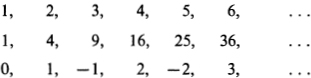
Collections which can be placed in 1-1 correspondence with the natural numbers we call countably infinite or denumerably infinite or enumerably infinite. To show that an infinite set is countable, we need only put its members into an infinite list, or 1-1 correspondence to the natural numbers as written above. A particular such list, or 1-1 correspondence to the natural numbers, we call an enumeration of the set. Examples of countably infinite sets are, besides the natural numbers themselves, the set of the positive integers, the set of the squares of the positive integers, and the set of all the integers, as we see from the following enumerations:

A countable set or denumerable set or enumerable set is a set which is either countably infinite or finite. Here we can describe a finite set as a set which can be put into 1-1 correspondence with an initial segment 0,. . ., n — 1 of the natural number sequence, possibly the empty segment (n = 0). This is equivalent to saying that a finite set is a set that has a natural number n as its “cardinal number”, as this use of natural numbers is commonly understood.¹²³

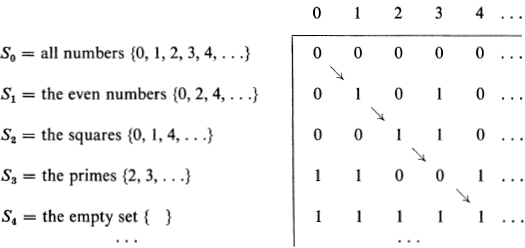
Another example of a countably infinite set is the set of the rational numbers. This is surprising, if one first compares them with the integers in the usual algebraic order. The points on the a – axis with integral abscissas are isolated, while those with rational abscissas are “everywhere dense”, i.e. between each two, no matter how close, there are always others. We can nevertheless enumerate them by the following device. We begin with the fact that each rational can be written as a fraction of integers with a positive denominator. We arrange all such fractions in an infinite matrix, thus:

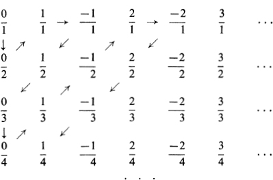
We can enumerate these fractions by following the arrows. Finally, we can go through that enumeration striking out each fraction which, interpreted as a rational number, is equal in value to one that has preceded it. This gives us the following enumeration of the rational numbers:

Another enumerably infinite set is the set of the real algebraic numbers, that is, the set of real numbers which are roots of algebraic equations (polynomial equations) in one variable x with integral coefficients, such as the equation

The general form of an algebraic equation of degree n (≥ 1) is

If we can enumerate the algebraic equations, we can enumerate the real algebraic numbers. For then, in the enumeration of the equations, we can replace each equation by its distinct real roots, which will be finitely many (at most as many as its degree), to obtain an “enumeration with repetitions” of the real algebraic numbers. Then the repetitions can be removed. The algebraic equations with integral coefficients can be enumerated by first noticing that we can without ambiguity simply write the exponents on the line with the rest of the symbols (thus: 4x5 – 17x3 +2x2 + 5 = 0). Then the equations become finite sequences of just fourteen different symbols:

The first symbol in an equation is not a 0. Now we can regard the fourteen symbols as the digits in a quattuordecimal number system, i.e. a number system based on 14 in the same way that the decimal system is based on 10. When we do so, each equation becomes an expression for a natural number, indeed a positive integer, in that system. Of course, not all natural numbers when written in the 14-system with the above symbols as the digits will read as algebraic equations. By leaving out the natural numbers which do not (closing up the “gaps”), we get an enumeration of the algebraic equations; that is, the algebraic equations can be listed in the order of magnitude of the positive integers which they become on interpreting their symbols as the digits in a 14-system.

We call the method just used for enumerating the algebraic equations the method of digits. We use it now to establish the following general principle.

(A) If all the members of a set S can be named unambiguously by nonempty finite sequences of {occurrences of) symbols from a given finite list of symbols or alphabet s₀,. . . , s_p-1, (or even from a countably infinite alphabet s₀, s_l, s₂,. . .), then the set S is countable.

In the case of a finite alphabet s₀,. . ., s_p-1, we could proceed as above (where p = 14 and s₀,. . . , s_p-1 are the fourteen symbols displayed), except for one contingency. After regarding a finite sequence of (occurrences of) S₀,. . ., S_p-1 as an expression for a natural number in the p-system with s₀,. . . , s_p-1 as the digits, we cannot tell from that number as a number how many initial s₀’s there were in the sequence. Thus, in the 14-system with the above digits, the same number is expressed by each of: 4x5 – 17x3 + 2x2 + 5 = 0 , 04x5 – 17x3 + 2x2 + 5 = 0 , 004x5 — 17x3 + 2x2 + 5 = 0 ,. . . . This ambiguity did not matter above, since we could and did exclude algebraic equations beginning with a 0. To avoid the ambiguity about the number of initial s₀’s when it does matter, we can instead regard the symbols s₀,. . ., S_p-1 as the digits for 1, . . . ,p in a p+l -system having a different symbol for 0 .

Notice that it does not matter whether the members of S have only one name each or several names using the alphabet s₀,. . ., s._p-1. If members of S may have several names, then when we eliminate the numbers not arising from names we can also eliminate all but the smallest number which we get from the several names of any one member of S.

The case of a countably infinite alphabet s₀, S₁, s₂,. . . can be reduced to the case of a finite alphabet by replacing each of the infinitely many symbols by a suitable combination of finitely many symbols. For example, we can pick two symbols a and b, and then replace s₀, s_l, s₂, s₃,. . . by a, ab, abb, abbb, . . . . Thereby e.g. the name s₀, s₃, s₁, s₁, becomes aabbbabab, from which without ambiguity we can recover s₀, s₃, s₁, s₁,. The method of digits can be applied to the new two-letter alphabet a, b; thus we can interpret aabbbabab as expressing a number in the ternary system with 0, a, b as the digits for 0, 1 , 2 . In particular cases, some other reduction of s₀, s₁, s₂,. . . to a finite alphabet may be more convenient to use.

Conversely: (B) If a set S is countable, its members can be named unambiguously by nonempty finite sequences of (occurrences of) symbols from a given finite alphabet. For, if S is infinite and a₀ , a_l , a₂ , ... is a particular enumeration of S , then a₀ can be named by 0 , a₁ by 1, a₂ by 2, . . ., using the 10 symbols 0, 1, . . . , 9. Briefly, each member a_i of S can be named by (the numeral for) its index i in a given enumeration a₀, a₁ a₂, . . . of S . Similarly, if S is finite.

Together, (A) and (B) should make it virtually obvious what sets are countable (i.e. finite or countably infinite). Other devices than the method of digits are often convenient for enumerating sets.

EXERCISES. 32.1. that, in the method of digits for a finite alphabet s₀,. . . , s_p-1, the names of the members of S are simply enumerated by taking all the one-letter names first, then all the two-letter names, then all the three-letter names, . . . , using alphabetic order within each group.

32.2. Use the method of digits to show the rational numbers countable. Give the first six rational numbers in the enumeration you obtain.

32.3. Show that the following sets are countable (use both the idea employed in the text for the rationals, and the method of digits):¹²⁴

(a) The ordered triples (a, b, c) of natural numbers, or of the members of any given countably infinite set.

(b) The finite sequences of such members.

(d) The finite sequences of finite sequences of such members.

32.4. Criticize the following argument: “Every real number x can be named unambiguously by an integer plus an infinite decimal fraction Only finitely many symbols 0,. . . , 9, . , + ,— are used in the names. Therefore by the method of digits (or (A)), the set of the real numbers is countable.”

§ 33. Cantor’s diagonal method . The results in § 32 on the application of the notion of 1-1 correspondence to infinite sets would perhaps have found their place in mathematical history as an interesting curiosity, not noticed before (or noticed earlier and forgotten) but leading nowhere especially, if it had turned out that each two infinite sets can be put into 1-1 correspondence. The fruitfulness of the idea of comparing infinite sets under 1-1 correspondences appears in that this is not the case. For, as we show next, there are uncountable or nondenumerable sets, i.e. infinite sets which cannot be put into 1-1 correspondence with the natural numbers.

We begin with the set of the one-place number-theoretic functions. These are the functions of one variable a ranging over the natural numbers with values also natural numbers. Examples are a², 3a+l , 5 (a constant function), a (the identity function), [] (the greatest integer ≤ ) , etc.¹²⁵

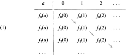
To prove the uncountability of the set of (all) these functions, suppose given an enumeration f₀(a), f₁(a), f₂(a) , ... of some one-place number-theoretic functions (not necessarily all). We shall thence construct a one-place number-theoretic function f(a) different from each function in the given enumeration. This will prove that the given enumeration cannot be an enumeration of all the one-place number-theoretic functions. To help us in visualizing the construction f (a), let us tabulate the sequences of values of the functions f₀(a), f₁(a), f₂(a) ... as the rows of an infinite matrix:

We define f(a) to be the function whose sequence of values is obtained by taking the successive values along the diagonal (indicated by the arrows) and changing each of them, say by adding 1 to it; thus,

This function does not occur in the given enumeration f₀(a), f₁(a), f₂(a), .... For, it differs from f₀(a) in the value taken for 0, from f₁(a) in the value taken for 1, and so on.

(Thus, if

then

but

To phrase the argument differently, suppose that the function f(a) were in the enumeration f₀(a), f₁(a) f₂(a), . . . ; i.e. suppose that for some natural number p,

for every natural number a. Substituting the number p for the variable a in this and the preceding equation,

This is impossible, since the natural number f_p(p) does not equal itself increased by 1.

The method we have just used is called Cantor’s diagonal method. By restricting the set of the functions to which we apply it, we next obtain some other examples of uncountable sets.

We can take just those one-place number-theoretic functions, each of which has only 0, 1,2, 3, 4, 5, 6, 7, 8, 9 as values and which does not have all its values 0 from some value on. Then the rows of the matrix (1) can be interpreted as the nonterminating decimal fractions for real numbers x in the interval 0 < x ≤ 1. Each such real number has just one such decimal expansion; e.g. . . . (we don’t use .75000 . . . = .75, which is “terminating”), , π — 3 = .14159 . . ., 2/3 = .66666 .... The alteration performed along the diagonal must not take us out of the class of functions considered. We can, say, change each value ≠ 5 to 5 and 5 to 6; thus

(If we obtain a real number x whose decimal expansion (necessarily nonterminating) starts out .55565 . . ..) This application of the diagonal method establishes that the set of the real numbers x in the interval 0 < x ≤ 1 is uncountable.

It follows almost at once that the set of all the real numbers is uncountable ( execises 33.1(a)).

It is interesting historically to note how Cantor’s discoveries in 1874 illuminated an earlier discovery of Liouville in 1844. Liouville constructed by a somewhat complicated special method certain transcendental (i.e. nonalgebraic) real numbers. Cantor’s diagonal method makes the existence of transcendental numbers apparent from only the very general considerations presented above. In fact, from any given enumeration of the algebraic numbers, particular transcendentals can be obtained by the diagonal method.

Finally, let us apply the diagonal method to the set of the one-place number-theoretic functions taking only 0 and 1 as values. Now we have no choice about the alteration performed along the diagonal. We must interchange 0 and 1; thus the “diagonal function” is defined by

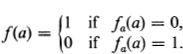
In this application, each function can be interpreted as describing the set of natural numbers at which the function value is 0; we call these functions the representing functions of these sets. We show some examples of sets of natural numbers at the left below, opposite the sequences of values of their representing functions.

For S₀ , S_l , S₂ , S₃ , S₄ , . . . as shown , the diagonal method gives the set S = {1, 2, 4, . . .} whose representing function starts out with the values 1, 0, 0, 1,0,.... Thus 0 is not a member of S, though it is of S₀ ; 1 is a member of S , though it is not a member of S₁; etc. So S is not any of S₀ , S₁ ,. . . . This application of the diagonal method shows that the set of all the sets of natural numbers is uncountable (in contrast to Exercise 32.3 (c)).

The sets shown in this section (including the exercise) to be uncountable can be put into 1-1 correspondence with one another (they are “equivalent”).¹²⁶ Closer examination of the diagonal method in § 34 will show that it gives us infinite sets which are neither countable nor “equivalent” to any of these uncountable sets.

EXERCISE 33.1. Show the following sets to be uncountable.

(a) The real numbers.

(b) The transcendental numbers.

§ 34. Abstract sets. Starting from these discoveries, Cantor developed a theory of abstract sets, in which he gave them a general setting and attempted to discuss sets of the most general sort.¹²⁷ We can give here only a brief indication of the theory of abstracts sets.¹²⁸

Cantor (1895 p. 481) defined a set thus, “By a ’set’ we understand any collection M of definite well-distinguished objects m of our perception or our thought (which are called the ’elements’ of M) into a whole.” We write “” to say that m is an element of M, or synonymously that m is a member of M or belongs to M; and “” to say that m does not belong to M.¹²⁹ Two sets M₁ and M₂ are the same (M₁ = M₂) if they have the same members. A finite set can be described by listing its members (the order being immaterial) in curly brackets; using dots, we can even suggest thus an infinite set. For example, {1,2, 3} is a set with three elements, and {0, 1, 2, . . .} is the set of the natural numbers. We say a set M₁ is a subset of a set M, and write M₁ ⊆ M (or M ⊇ M₁), if each member of M₁ is a member of M. For example, the three-element set {1, 2, 3} has eight subsets

The first { } is the empty (or vacuous) set (often written ø ), the next three are unit (i.e. one-element) sets, and the last is the improper subset of {1, 2, 3}.

The cardinal number is a notion which we “abstract” from M and the other sets which can be put into 1-1 correspondence with M. Thus a child gets his concept of “two” by abstracting from two parents, two ears, two apples, two kittens, etc. What “two” itself is may not worry him. Cantor wrote, “The general concept which with the aid of our active intelligence results from a set M, when we abstract from the nature of its various elements and from the order of their being given, we call the ’power’ or ’cardinal number’ of Af.” This double abstraction suggests his notation “M” for the cardinal of M. Frege 1884 and Russell 1902 defined M as the set of all the sets N which can be put into 1-1 correspondence with M; this gives a place to the cardinals themselves as objects of a universe whose only members are sets. To put this in terms that were elaborated in § 30, let us say M is equivalent to N, and write M ~ N, if M can be put into 1-1 correspondence with N. Then ~ is an equivalence relation (i.e. it is symmetric, reflexive and transitive); and is the equivalence class to which M belongs under ~ within a universe of sets (cf. (B) in § 30).

Whatever one’s ontology of the cardinals, if and only if M ~ N.

For any set M, we write “2^M” as a notation for the set of all the subsets of M.

In our present notation, our last result in § 33 is that 2^M is uncountable, or when M = {0, 1, 2, . . .}. The reasoning applies similarly to any set M to show that Let us repeat the reasoning for the case M = {1,2, 3}. Given any set M₁ ⊆ 2^M which is in 1-1 correspondence with M itself, the diagonal method leads us to a subset of M (i.e. a member of 2^M) not belonging to M₁ Thus, if M₁ = {{2}, {2, 3}, {1, 2}}, the matrix is as follows:

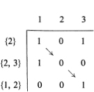
Interchanging 0 and 1 on the diagonal, we are led to {1, 3}, which is a member of 2^M (2^M has the eight members displayed above) but not of M₁ If instead M₁ = {{1,2, 3}, {1}, {3}}, we get {2}, which again is not in M₁; etc. Of course, since 2^M has eight members, i.e. , while , we can say we already knew that for M = (1, 2, 3}, as part of what we are taking for granted about the natural number sequence. However, this and the concluding example in§ 33 with M = {0, 1, 2,. . .} are two illustrations of the general proof that, for each set M, .

This result can be given a stronger form. First, we define (or ) to hold exactly if M is equivalent to some subset of N but N is equivalent to no subset of M (i.e. if there is a set N₁ such that M ~ N₁ ⊆ N but there is no set M₁ such that N ~ M₁ ⊆ M). Here it is necessary to verify that the result is independent of which sets M and N with the respective cardinals and we use, or in the terminology of § 30 of which members M and N we pick from the two equivalence classes and (Exercise 34.1). We see almost at once that the order relation < between cardinals is irreflexive (i.e. ) and transitive (i.e. if and then ) (Exercise 34.2).

As we already remarked in§ 32 assuming familiarity with the natural number sequence, the natural number n is the cardinal of the initial segment 0, . . .n — 1 of the natural numbers. Consequently, Cantor’s definition of the order relation < between any two cardinals applies in particular to the natural numbers as cardinals. It can be shown (though not without some trouble) that this order relation < between the natural numbers as finite cardinals coincides with the familiar one which we have been taking for granted.¹³⁰

By only slight refinements of the argument given above, we can establish Cantor’s theorem: (C) For each set M,

Another easily proved theorem concerns the union ∪M of a set M whose members are sets. ∪M has as its members each of the objects which is a member of a member of M. For example, if M = {{2}, {2, 3}, {2, 5}}, then ∪M = {2, 3, 5}. The theorem is: (D) If M is a set of sets containing none of greatest cardinal (i.e. to each member A of M there is a member ′ of M with ), then for each member A of M.

We adopt the notation (read “aleph null” or “aleph zero”) for the cardinal of the set of natural numbers. Then for each natural number n, This follows from (D) with n = and the fact that the cardinal order of the natural numbers is also their usual order.

Also we write as “”. For M finite, this is consistent with the usual arithmetic; e.g. we saw that when .

The foregoing results give the existence of the following ascending series of cardinals

while by (D) there is a still greater cardinal after all of these, and so on indefinitely. Thus, by applying the idea of comparing sets by one-to-one correspondences, Cantor discovered that there is not simple one infinity, but a whole hierarchy of different infinite (or “transfinite”) cardinals.

EXERCISES. 34.1. Justify the definition of “” by showing that, if M ~ M′ and N ~ N′₁ then (α) holds if and only if (α′) holds :

(a) For some N_l, M ~ N₁ ⊆ N; but for no M_l, N ~ M₁ ⊆ M.

(α′) For some N_l, M ′ ~ N₁ ⊆ N′; but for no M_l, N′ ~ M₁ ⊆ M′.

34.2. Show that the relation is irreflexive and transitive.

34.3*. Prove (C) and (D).

34.4. (a) What is the cardinal of the set in Exercise 33.1 (c)? (b) What is the cardinal of the set of the one-place logical functions when the domain is the sets of natural numbers ?

§ 35. The paradoxes. The relation between Cantor’s set theory and mathematics was like the course of true love; it never did run smooth.

Cantor’s set theory deals with “actual” or “completed” infinities. At the beginning there was great resistance to this by the mathematical public, stemming in part from the famous dictum of Gauss (1831): “I protest. . . against the use of an infinite magnitude as something completed, which is never permissible in mathematics: one has in mind limits which certain ratios approach as closely as desirable while other ratios may increase indefinitely.” (Werke VIII p. 216.) Gauss had in mind infinite magnitudes, while Cantor’s theory employs infinite collections.

Just when Cantor’s ideas were well on the way toward winning acceptance from most mathematicians, in the 1890’s contradictions appeared in the upper reaches of his set theory. Nevertheless, since then set theory (suitably adapted) has increased its place in mathematics, while the paradoxes have focussed attention on the foundations of set theory and of mathematics generally.

The Burali-Forti paradox which appeared in 1897 (but was known to Cantor in 1895) arises in Cantor’s theory of ordinal numbers, which we have not discussed.¹⁸³

Russell’s paradox 1902a concerns the set of all sets which do not contain themselves. Call this set S. Suppose (a) S contains itself. Then by the definition of S, S does not contain itself. So by reductio ad absurdum (rejecting the supposition (a)), we have proved: (b) S does not contain itself. But then by the definition of S: (c) S does contain itself. Together (b) and (c) constitute a proved contradiction, or paradox.

Russell in 1919 gave the following popularized version: The barber in a certain village shaves all and only those persons in the village who do not shave themselves. Question: Does he shave himself?

We now give in detail a third paradox of the theory of sets, the Cantor paradox (found by him in 1899). Let T be the set of all sets. Now 2^T is a set of sets, and hence 2^T ⊆ T. By the definition of < for cardinals (§ 34), if M ⊆ N then (Why?) So . But by Cantor’s theorem (C), . Thus we have a contradiction.

One may try to dismiss this by saying that the set T of all sets does not constitute a set. Then in Cantor’s theorem “For each set M, ”, what is the range of the variable M (what we called the domain D in Chapter II)?

Of a somewhat different type is the Richard paradox (Jules Richard, 1905), which runs as follows.

By a “phrase” we shall mean any finite sequence each of whose members is either a blank or one of the twenty-six letters of our alphabet (with a blank not first or last). Thus, “abracadabra”, “of cabbages and kings”, “the square of a”, and “xtu rlbp” are phrases. We can enumerate the phrases by the method of digits (§ 32), using a 27-digit or 28-digit number system to represent the natural numbers. Certain phrases, such as our example “the square of a”, describe in the English language one-place number-theoretic functions. We now strike out from our enumeration of all the phrases those which do not describe such functions; thereby we obtain an enumeration P₀, P₁, P₂,.. . of the phrases which do. Say the functions described are f₀(a),f₁(a), f₂(a),. . ., respectively.

Now consider the following phrase: “the function whose value for each natural number a is obtained by adding one to the value for a of the function described by the phrase corresponding to a in our enumeration of the phrases which describe one place numbertheoretic functions”. In this phrase, we could replace the last part “in our enumeration of the phrases which describe one place numbertheoretic functions” by a detailed description of the exact construction of the enumeration, and so obtain from the whole another phrase P fully describing the same function.

This phrase P describes a number-theoretic function, namely

Hence P occurs in the enumeration P₀, P₁, P₂,. . .. This is impossible, since the function described by P differs from that described by P₀ in its value for a = 0, from that described by P₁ in its value for a = 1, from that described by P₂ in its value for a = 2, and so on. Otherwise expressed: Since the phrase P occurs in the enumeration P₀, P_l, P₂,. . ., it is P_p for some p. Then

A contradiction arises by substituting p for a in this and the preceding equation. (In Richard’s original version, real numbers were used instead of one-place number-theoretic functions.)

This paradox is closely connected with the facts that, on the one hand, only a countable infinity of number-theoretic functions are describable in a given language (because the set of all the phrases in the language is only countably infinite, § 32), while, on the other hand, the set of all the number-theoretic functions is uncountable (by Cantor’s diagonal method, § 33).

A similar paradox is due to G. G. Berry (in Russell 1906 p. 645). Consider the expression “the least natural number not nameable in fewer than twenty-two syllables”. This expression names a definite natural number, say n, since each nonempty set of natural numbers (in this case, the set of natural numbers not nameable in fewer than twenty-two syllables) has a least element. By its definition, n is not nameable in fewer than twenty-two syllables. But our expression naming n has in fact exactly twenty-one syllables!

These modern paradoxes are related to the paradox of “The Liar”, which comes from antiquity.¹³¹ The following statement is attributed to the Cretan philosopher Epimenides, sixth century B.C. “All Cretans are liars”. Let us suppose that by “liar” Epimenides meant a person who never tells the truth.

Suppose his statement is true; then by what it says and by his being a Cretan, it is false, which is a contradiction. So by reductio ad absurdum, the statement is not true, i.e. it is false. This means that at some time some Cretan has told the truth or eventually some Cretan will tell the truth. This, however, should be a matter for the historian to decide; it should not be demonstrable on logical grounds only, as we appear to have demonstrated it.

The direct form of the paradox of “The Liar” was given by Eubulides in the fourth century B.C. We can give it as follows: “The statement I am now making is a lie.” One sees directly that the quoted statement cannot be true and that it cannot be false.

In the ancient “dilemma of the crocodile”, a crocodile has stolen a child, but offers to return the child to its father, if the father can guess whether or not the crocodile will return the child. If the father guesses that the crocodile will not return the child, the crocodile is in a dilemma.

A missionary, fallen among cannibals, discovers that he is about to become their supper. They offer him the opportunity to make a statement, under the conditions that, if the statement is true, he will be boiled, and if it is false, he will be roasted. What should the missionary say?

Cantor’s set theory, as historically it first arose and as we met it in §32- §34, is called “naive” set theory. In using Cantor’s “definition” of a set (§ 34), Cantor and we were guided only by our imagination in deciding which objects are sets.

Cantor’s and the other paradoxes of set theory show the difficulties inherent in the attempts to develop the theory on an intuitive basis starting from Cantor’s definition of set. These difficulties pose the problem how to modify set theory so that contradictions do not arise. In fact, the problem goes further, and forces us to ask ourselves wherein we were deceived by methods of constructing and reasoning about objects which had seemed convincing before they were found to eventuate in paradoxes. Complete agreement among mathematicians on the cause of the paradoxes and the cure has not been attained yet (1967), and it seems problematical that it ever will.

In the remainder of this section, we indicate briefly the least radical kind of reformulation of mathematics toward avoiding such paradoxes as the Burali-Forti, Cantor’s and Russell’s. (Ramsey 1926 classified the known paradoxes into two sorts, one now called “logical” including the three just mentioned, the other “epistemological” or “semantical” including Richard’s, Berry’s and “The Liar”.)

This reformulation of mathematics begins with the observation that the paradoxes of set theory (the logical paradoxes) are associated with using “too large” sets, such as the set T of all sets in Cantor’s paradox. Since free use of our conceptions starting with Cantor’s definition of set led to the difficulty, Zermelo proposed in 1908 to restrict the sets to those provided by a list of axioms. These axioms are drawn up so that there is no apparent means to derive the known paradoxes from them. On the other hand, the axioms do suffice for the deduction of the usual body of classical mathematics, including abstract set theory short of the paradoxes.

We give now, in our words, the list of seven axioms or principles which appear in Fraenkel 1961 with the pages where they appear.¹³² (It is not intended that the student, so far as this course is concerned, should learn these axioms. We give them here to exemplify what sort of axioms are used.) Choosing this particular list of axioms has the advantage that the excellent expositions in Fraenkel 1961 and in Fraenkel and Bar-Hillel 1958 are built around them. Another axiomatic treatment is in Bernays and Fraenkel 1958.

(I) (Axioms of extensionality, p. 14.) Two sets A and B are equal if (and only if) they contain the same members; i.e. A = B~(A ⊆ B and B⊆ A).

(II) (Axiom of subsets, p. 16.) Given a set A and a predicate P(x) meaningful for the members of A (i.e., for each either P(x) is true or P(x) is false), there exists the set containing exactly those members of A for which P(x) is true. (This axiom is also called the “axiom of selection”, the “axiom of segregation” or the “Aussonderungs-axiom”.)

(III) (Axiom of pairing, p. 18.) If a and b are different objects, there exists the set {a, b} containing exactly a and b .

(IV) (Axiom of union, p. 20.) Given a set S of sets, there exists the set ∪S containing just the members of the members of S .

(V) (Axiom of infinity, p. 32.) There exists at least one infinite set: the set {0, 1,2,...} of the natural numbers. (Fraenkel used {1, 2, 3,. . .}.)

(VI) (Axiom of the power set, p. 72.) Given a set A, there exists the set 2^A whose members are all the subsets of A.

(VII) (Axiom of choice, p. 90.) Given a disjointed set S of nonempty sets, there exists a set C which has as its members one and only one element from each member of S. (S is disjointed if no two distinct members of S have an element is common.)

A form of the axiom of choice was first explicitly noted as an assumption in Zermelo’s proof of his “well-ordering theorem” 1904,1908a, from which it follows that each two cardinal numbers and are comparable (i.e. that either or or ). The form given here, which is Russell’s “multiplicative axiom” 1906a, suffices for the derivation of Zermelo’s form (and vice versa).

The axiom of choice has been the subject of much research with a view to minimizing its use, singling out its consequences, or (Godel 1938, 1939, 1940) defending it as an assumption which can be added to the other axioms of set theory without entailing a contradiction if the other axioms by themselves lead to no contradiction.¹³³ In 1963-4 Cohen showed that instead the negation of the axiom of choice can be added consistently (detailed exposition in 1966). Another treatment is in Scott 1966.

At one point these axioms (as did the axioms given by Zermelo in 1908a) lack definiteness. This is in (II), where the notion of a predicate P(x) meaningful for elements is incorporated. This lack of definiteness was first remedied by Fraenkel 1922 and somewhat differently by Skolem 1922-3. What is required is a specification of a class of admissible predicates P(x). In Skolem’s method, the rules for constructing the P(x)′s are formulated simply in the process of specifying the symbolism of the language in which the axioms are stated.

The specification of the symbolism of a language, which is necessary for the purpose of being exact in logical deduction, must really be presupposed for the rigorous treatment of logic as in Chapters I—III above. The semantical paradoxes (Richard’s, Berry’s, “The Liar”) show that care is necessary in this. That is, the language of a mathematical theory must be subjected to rules governing the formation of propositions somewhat akin to the rules listed above governing the existence of sets. We shall deal further with this.

In some systems of axiomatic set theory (particularly Godel’s, 1940) two sorts of collections are considered explicitly, collections called “sets” which can not only possess members but also be members of collections, and others called “classes” which may not be taken as members of collections. Each “set” is a “class”. The collection of all “sets” constitutes a “class”; but we are stopped from obtaining the Cantor paradox because this “class” is not a “set”.

In the definition of validity in the predicate calculus (§ 17), we simply said the domain D is to be a “nonempty set or collection”. That was before we were ready to talk about a distinction between “sets” and “classes” in the present sense. We can get a little more leeway now for model theory by allowing D to be a nonempty “class”. For in the notion of validity, we do not need to take D as a member of anything. The difficulties which ensue when “too large” collections are treated as members are not involved in just using a collection as the range of variables. This gives an answer to the question raised above of what the domain D can be for set theory itself (where we asked about the range of M in Cantor′s theorem, ). (Except when we refer explicitly to this passage, “class” will continue in this book to be a synonym for “set” as in ordinary usage.)

§ 36. Axiomatic thinking vs. intuitive thinking in mathematics. Partly in connection with the broader aspects of the problem posed by the paradoxes (§ 35), we inquire now into the nature of mathematics and the scope of mathematical methods.

The axiomatic-deductive method in mathematics is known to us from Euclid’s “Elements” (c. 330-320 B.C.), although there is a tradition that credits Pythagoras (sixth century B.C.) with the introduction of the method. By use of it, the body of geometrical knowledge was systematized. Euclid’s axiomatic system may be described roughly thus: “definitions” of certain primitive terms, such as “point”, “line”, “plane” are given, which are intended to suggest to the reader what is meant by those terms; certain propositions concerning the primitive terms, felt to be acceptable as immediately true on the basis of the meanings suggested by the definitions, are taken as axioms or postulates; then other terms are defined in terms of the primitive ones; and other propositions, called theorems, are deduced by logic from the axioms. Axiomatics such as Euclid’s, in which meanings are given to the primitive terms from the outset, is called material axiomatics.

One of Euclid’s postulates seemed less evident than the rest, the fifth postulate or “parallel postulate”.¹³⁴ He used this in proving the theorem that, through a given point P not on a given line I, exactly one line can be drawn parallel to I (i.e. not meeting / in a point). Efforts were made from Euclid’s time on to prove this postulate from the others as a theorem. We now know these efforts could not succeed.

For, Lobatchevski in 1829 and Bolyai in 1833 worked out a system of geometry in which, through a given point P not on a given line I, infinitely many lines parallel to I can be drawn. It is apparent that the meanings of Euclid’s primitive terms in terms of physical space do not enable one to decide whether Euclid’s parallel postulate is true or the contrary postulate of Lobatchevsky and Bolyai. The differences in the resulting geometries may be too small to show up in any measurements we can make in the portion of space accessible to us, just as in some other times people have thought the earth flat from the portion of it they could see.

So whether a proposition of Euclidean geometry is exactly true must be a property of the geometry as a logical system. But if Euclidean geometry is a valid logical structure, so is the Lobatchevskian geometry. For, as Felix Klein pointed out in 1871, the axioms of the plane Lobatchevskian geometry are all true when the primitive terms in them are reinterpreted so that “plane” is taken to mean the interior of a given circle in the Euclidean plane, “point” means a point inside this circle, “line” means a chord of this circle, and distances and angles are computed by formulas due to Cayley 1859. (Another such Euclidean model, applicable to a bounded portion of the non-Euclidean plane, was given in 1868 by Beltrami, who reinterpreted line segments as segments of shortest paths between points, or “geodesies”, on a “surface of constant negative curvature”.)

In these models, we may observe that something new has been done with the axioms, not to be found in the earlier axiomatic thinking: the meanings of the primitive terms have been varied, holding the deductive structure of the theory fixed. Thus formal axiomatics arose, in which the meanings of the primitive terms, instead of being specified in advance, are left unspecified for the deductions of the theorems from the axioms. One is then free to choose the meanings of the primitive terms in any way that makes the axioms true. We have been representing this standpoint in our definition of “valid consequence” in model theory (§§ 7, 20). Especially in modern algebra, it has proved very fruitful to develop the consequences of systems of axioms regarded formally, such as the axioms of abstract group theory (cf. § 39). The results deduced from the axioms of group theory, while leaving unspecified the set of elements and the multiplication operation, constitute a body of theory ready-made for diverse applications.

In formal axiomatics, the system of axioms may be investigated for such properties as the independence of one axiom from the others (by seeking an interpretation of the primitive terms which makes that axiom false and the others true), categoricity (i.e. that the elements in any two interpretations can be put into 1-1 correspondence preserving all properties), etc.¹³⁵

In this approach to axiomatics some questions arise. Why do we choose the axioms we do, and why should the resulting systems interest us ? The answer is evidently that we may apply the resulting theory to systems of objects provided from outside the axioms by an interpretation of the primitive terms. Sometimes essentially different interpretations are possible (the axioms are then not categorical, but ambiguous) e.g. this is the case for the axioms for abstract groups. We should not wish to employ a system of .axioms satisfied under no interpretation; such a system we call vacuous. One of the problems in formal axiomatics is to show axiom systems non-vacuous. However, a system of objects used as an interpretation is often drawn from some other axiomatic theory; then we have a regress, which merely brings us to the question of the significance of that axiomatic theory instead. If at no stage is an application made outside of formal axiomatics, the whole activity must appear to be futile. We therefore conclude that, if we are not to adopt a mathematical nihilism, formally axiomatized mathematics must not be the whole of mathematics. At some place there must be meaning, truth and falsity. At the very least, when we say that in a given formal axiomatic theory a certain proposition is a theorem, we must believe this is true, i.e. that the proposition does follow from the axioms, though whether the proposition itself is true is being left out of account, since in formal axiomatics the deductions are carried out in advance of assigning meanings to the primitive terms (or disregarding any such assignment).

As a further illustration of a mathematical proposition which is not intended to be asserted merely as a formal but meaningless consequence of axioms, consider the theorem (proved in number theory) that, for given integers a, b, c, we can find out whether or not integers x and y exist such that ax + by + c = 0, i.e. the theorem that there is a method of deciding whether or not the equation ax + by + c = 0 (a, b, c integers) is solvable in integers. Although the theory of the integers may have been established axiomatically, this proof is intended to mean that, for any particular a, b, c, we can discover whether or not there are solutions. A student who could merely give a proof from axioms of the theorem that one can find out whether there are solutions or not, but could not do a problem, in which he found out, would not have acquired what the teacher intended to teach. Nevertheless, he would be doing all that should be asked of him if the theorem (that one can find out) were intended only in the sense of formal axiomatics.

As the least drastic method of meeting the situation posed by the paradoxes, we described axiomatic set theory at the end of § 35. Here the axiomatics is to be understood in the formal sense, unless one is to try to retain an intuitive conception of sets, which it was presumed was exactly what the axioms were intended to supplant. However the present considerations show that the resort to a formal axiomatic theory, though it may offer considerable advantages, leaves open such problems as why the axioms are significant and whether or not they apply to any system of objects not merely similarly postulated as existing for some other formal axiomatic theory.

Hilbert undertook to deal with these problems. He admitted that classical mathematics (i.e. the familiar mathematics using classical logic) contains much that goes beyond what is clearly meaningful and justifiable on intuitive grounds, as indeed mathematicians generally were made to realize when in set theory they went too far and encountered paradoxes. But he proposed to save classical mathematics (short of paradoxes) by a program which we can roughly describe as follows. Classical mathematics should be formulated as a formal axiomatic theory, and then the theory should be shown to be consistent, i.e. free from contradiction.

Before this proposal of Hilbert, first made in 1904, but not seriously undertaken by him and his co-workers until after 1920, consistency proofs had been given for formal axiomatic theories by means of a model or interpretation, in which all the axioms are found to be true when the primitive terms are interpreted in terms of another theory. We saw an example of this above, by which the non-Euclidean plane geometry of Lobatchevsky is shown to be consistent if Euclidean geometry is consistent.¹³⁵ In each case, a proof of consistency by a model only shows the theory consistent if another is. By Rene Descartes’ method of analytic geometry 1619, the consistency of geometries generally is reduced to that of the theory of real numbers, i.e. to analysis. But how is one to establish the consistency of analysis? Certainly not by using a geometrical model; this would be a vicious circle. Nor, according to Hilbert and Bernays 1934, by appeal to the physical world. For limitations of our measurements in the physical world prevent us from saying that a continuum is actually given by experience; rather it is an idea we obtain by extrapolating or idealizing what is actually given.¹³⁶

So Hilbert’s proposal to prove classical mathematics as embodied in a formal system consistent called for a new method in place of the method of giving a model. This method consists in a direct application of the idea of consistency, namely, that there be no contradiction or paradox consisting of two theorems, one of which is the negation of the other. To show that this cannot happen, Hilbert proposed to make the proofs in the axiomatic theory the object of a mathematical investigation, called metamathe-matics or proof theory. Of course, such a demonstration of consistency would be relative to the methods used in the metamathematics. Hilbert therefore aimed to use in his metamathematics only methods, which we call “finitary”, that are intuitively convincing. Specifically, these methods should avoid using an “actual” or “completed” infinity. Hilbert’s new approach avoids the completed infinite in the statement of the problem of proving consistency. For there is only a countable infinity of proofs in a given theory, and the consistency proposition only concerns any pair of proofs, not the set of all proofs as a completed object. (What the theory is supposed to be about may be much less elementary.) So it seemed not unreasonable to hope that the problem of consistency, now that it was stated in finitary terms, might be solved by finitary methods.

In § 37- §39 we shall take a closer look at how parts of mathematics can be made into formal axiomatic theories and studied in metamathematics.

Brouwer was the champion of intuitive thinking in mathematics, as Hilbert was of axiomatic thinking. Brouwer’s and Hilbert’s approaches may also be called “genetic” (or “constructive”) and “existential”, respectively.

According to Weyl 1946, “Brouwer made it clear, as I think beyond any doubt, that there is no evidence supporting the belief in the existential character of the totality of all natural numbers .... The sequence of numbers which grows beyond any stage already reached by passing to the next number, is a manifold of possibilities open towards infinity; it remains forever in the status of creation, but is not a closed realm of things existing in themselves.”

While Hilbert proposed to shore up the structure of classical mathematics by a consistency proof, Brouwer was ready to abandon those parts of mathematics in which mathematicians had been carried away by words that had outrun clear meanings. Brouwer proposed instead to develop an “intuitionistic” mathematics, which would go only as far as intuition would lead it. For Brouwer, the systems* of objects for mathematics should be generated by some principles of construction, not brought into existence all at once as sets satisfying a list of axioms.

Since Brouwer took only the “uncompleted” or “potential” infinite as intuitive, he declined to accept logical principles which require for their justification a conception of infinite sets as completed. So, in a paper entitled “The untrustworthiness of the principles of logic” 1908, he challenged the assumption that the laws of classical logic have an absolute validity, independent of the subject matter to which they are applied. Particularly, he criticized the law of the excluded middle, P V ¬p Consider a predicate P(x) where x ranges over some set D. Applied to ∃xP(x) as the P, the law says that either there is an x in D such that P(x) or there is no x in D such that P(x); in symbols: ∃xP(x) V ∃xP(x). In case D is a finite set (and P(x) is a predicate such that, for each value x in D, we can test whether P(x) holds or not), Brouwer finds ∃xP(x) V ¬ ∃xP(x) true. For, we can find out whether ∃xP(x) or ¬ ∃xP(x) by testing, for each member x of D in turn, whether or not P(x) holds for that x. Since D is finite, this process will (in principle) terminate. But if D is an infinite set, say a countable one, such as the set of the natural numbers, the testing process cannot humanly be completed. If we are lucky, we may part way through the testing find an x such that P(x). But if there is no such x, or if such an x comes too late and doomsday comes too soon, we could search till doomsday and still not have an answer to our question. Accordingly Brouwer finds no ground for taking ∃xP(x) V ¬ ∃xP(x)to be always true, when D is infinite. Quoting from Weyl 1946, “According to his view and reading of history, classical logic was abstracted from the mathematics of finite sets and their subsets. . . . Forgetful of this limited origin, one afterwards mistook that logic for something above and prior to all mathematics, and finally applied it, without justification, to the mathematics of infinite sets.”

Brouwer’s path, like Hilbert’s as we shall see, was beset with difficulties. An intuitionistic mathematics was developed (beginning in 1918), which in part falls short of classical mathematics in the results obtained, in part takes a different direction. In parts common to classical and intuitionistic mathematics, the intuitionistic (or “constructive”) proofs, though often harder, often give more information. To prove an existence statement ∃xA(x) an intuitionist insists that it be shown how to find an x such that A(x). An “indirect proof” by showing that the assumption ¬ ∃xA(x) leads to contradiction is not accepted by him as showing ∃xA(x) it establishes only ¬¬∃xA(x).¹³⁷

Now we touch on the controversy between Brouwer and Hilbert.

Brouwer argued that, even if Hilbert should succeed in giving a consistency proof for classical mathematics, that would not make classical mathematics correct. Thus he wrote in 1923, “An incorrect theory which is not stopped by a contradiction is none the less incorrect, just as a criminal policy unchecked by a reprimanding court is none the less criminal.” Hilbert retorted in 1928, “To take the law of the excluded middle away from the mathematician would be like denying the astronomer the telescope or the boxer the use of his fists.” This controversy between the “formalists”, represented by Hilbert, and the “intuitionists”, represented by Brouwer, led eventually to the acknowledgement by the intuitionists that Hilbert’s program would be unobjectionable if and only if the formalists refrain from taking a consistency proof as justification for attaching a real meaning to those parts of mathematics which the intuitionists reject as having no intuitive basis (Brouwer 1928).

It remains then for the formalist to explain, after having admitted that classical mathematics goes beyond intuitive evidence, how nevertheless its nonintuitionistic parts can be of value. Addressing himself to this problem, Hilbert 1926, 1928 drew a distinction between real statements which have an intuitive meaning, and ideal statements (involving the completed infinite) which do not. It is a common device of modern mathematics to adjoin “ideal elements” to a previously constituted system in order to achieve theoretical objectives, such as to simplify the theorems, comprehend them under a more unified viewpoint, etc. An example occurs in projective geometry, where a line at infinity is adjoined to the finite part of the plane so that any two (distinct) parallel lines intersect in a point of that line. Thereby the exception for parallel lines to the “incidence relations” between points and lines is removed. Thus, in projective geometry, not only do each two distinct points contain a unique line (which passes through both), but dually each two distinct lines contain a unique point (in which they intersect). Hilbert argued that just this kind of theoretical gain is achieved by adjoining the ideal statements to the real statements in classical mathematics; it is through this procedure that classical mathematics achieves its power and elegance.

In this way, mathematics becomes a theoretical construction in which, Hilbert says, it should not be expected that each separate statement should have a real meaning, any more than that each proposition in a system of theoretical physics should be capable of immediate experimental verification; in the latter case, it is the theory as a whole that is tested against reality.

A concrete example of the theoretical gain obtained by going through ideal statements in the process of proving real statements is provided by analytic number theory, in which theorems about integers are proved via the theory of real or complex numbers. Many propositions of elementary number theory have been proved thus, which either we do not know how to prove, or can establish only by much more complicated proofs, if only nonanalytic methods are used.

§ 37. Formal systems, metamathematics. In § 36, we discussed formal axiomatics, stressing that the primitive terms are to be treated as meaningless for the purpose of deductions from the axioms by logic; i.e. either they have been assigned no meanings, or the meanings they have been assigned are to be left out of account. If they had meanings which have to be taken into account, this would amount to saying that the theorems depend not only on the properties of the primitive terms expressed by the axioms, but also on further properties which enter through the use of the meanings. But then those further properties should be stated as additional axioms.

Euclid in his “Elements” failed to state in his “axioms and postulates” all the properties he used. Figures accompany many of his proofs. It had long been taken for granted that the figures are inessential to the proofs, serving only to make it easier to discover them or to follow them or to remember them. But they do in fact sometimes introduce information that is used.

This has been dramatically illustrated by devising “proofs” of “false” theorems, such as that every triangle is isosceles.¹³⁹ There is nothing different in these “proofs” from proofs given in Euclid except the use of slightly distorted figures.

The “hidden” assumptions of Euclid have been brought into the light in modern times, and stated as axioms by Pasch 1882, Hilbert 1899 and others. Thus Hilbert’s axioms include the following, adapted from Pasch : If a line in the plane of a triangle not passing through a vertex cuts a side, it cuts one or the other of the remaining two sides. Our figures do come out this way; but nothing in Euclid’s text enables us to prove that they must. Hilbert’s “Grundlagen der Geometrie” 1899 gives an elegant treatment of Euclidean geometry from the standpoint of formal axiomatics, with all assumptions explicitly stated.

Now in formal axiomatics, while the primitive terms are to be meaningless, in carrying out the deductions by logic the meanings of the ordinary words are used. However, we have seen that theories may differ in their logic as well as in their mathematical assumptions. So, to make it perfectly explicit what the theorems of a theory are to be, we should carry out the step for all the words which is carried out in formal axiomatics for the primitive terms; i.e. we should divest them of meaning for the purpose of deductions, and carry out the deductions entirely by stated rules applying only to the form of the sentences. The logic used in the deductions in formal axiomatics must be represented in part by these rules, but may in part also be provided by logical axioms.

To carry out such a complete formalization would not be practicable if the theory were kept in an ordinary language such as English. For, the word languages have irregularities and ambiguities which would greatly complicate the task.

Indeed mathematics has in the entire modern period profited greatly by using special symbolisms, though it has customarily left parts of its sentences, including the parts involved in logical deduction, in ordinary language. The symbolic equation not only represents a great economy in writing, but presents an opportunity for manipulations (such as transposing: e.g. x + 5 = 2 gives x = 2 — 5 and x = — 3), which, though justified by the meanings, are in practice usually carried out speedily without stopping to think through the justifications. This is indeed a semi-formal kind of reasoning, which greatly increases the power of modern mathematics.

The complete formalization which we now desire, for Hilbert’s and other purposes, is obtained by combining the symbolization prevalent in modern mathematics with the symbolic treatment of logic available from the work of Boole, Peirce, Frege, Whitehead and Russell, and others. Using these two ingredients, we construct a completely symbolic language for the theory we wish to formalize. We specify both its syntax (by “formation rules”) and its logic (by “ive rules” or “transformation rules”).²⁸ The result we call a formal system or formalism or logistic system. This method of making a theory explicit is sometimes called the logistic method.

To discuss a formal system, which includes both defining it (i.e. specifying its formation and transformation rules) and investigating the result, we operate in another theory or language, which we call the metatheory or metalanguage or syntax language. In contrast, the formal system is the object theory or object language. The study of a formal system, carried out in the metalanguage as part of informal mathematics, we call metamathe-matics or proof theory.

For the metalanguage we use ordinary English and operate informally, i.e. on the basis of meanings rather than by formal rules (which would require a metametalanguage for their statement and use). Since in the metamathematics English is being applied to the discussion only of the symbols, sequences of symbols, etc. of the object language, which constitute a relatively tangible subject matter, it should be free in this context from the kind of lack of clarity that was one of the reasons for formalizing.

Since a formal system (usually) results by formalizing portions of existing informal or semiformal mathematics, its symbols, formulas etc. will have meanings or interpretations in terms of that informal or semiformal mathematics. These meanings together we call the (intended or usual or standard) interpretation or interpretations of the formal system.¹⁴⁰ If we were not aware of this interpretation, the formal system would be devoid of interest for us. But the metamathematics, to accomplish its purpose, must study the formal system as just itself, i.e. as simply a system of meaningless symbols, and may not take into account its interpretation. When we speak about the interpretation, we are not doing metamathematics.

Furthermore, as we saw in § 36, for Hilbert’s program the methods used in metamathematics must be ones, called “finitary”, which are intuitively convincing.

Now we relate the present terminology to that used in Part I. We do not consider a language, taken as an object of study, to be a “formal system” unless it is a symbolic language (not a part of a word language, like English) and unless axioms and rules of inference are specified for it (not simply model-theoretic concepts, like “valid” and “valid consequence”). We do not refer to a language used in studying an object language as the “metalanguage” or “syntax language” unless in it only finitary methods are used (though some authors do). Thus “object language” and “observer’s language” as used in Part I are broader terms than “formal system” and “metalanguage”.

In Part I, we used “proof theory” a little loosely compared to Hilbert’s intended sense, to which we shall now adhere. For, we had not actually specified a symbolic language there.¹⁴¹

If we supply suitable definitions (referring to a symbolic language) of “prime formula” or “atom” for the propositional calculus, and of “prime predicate expression” or “ion” for the predicate calculus (or with functions § 28, also of “prime function expression” or “meson”), then using them as the basis for the definition of “formula” in § 1 or § 16 or § 29 (or of “term” and “formula” in § 28 or § 29), we get formal systems of propositional calculus and of predicate calculus without or with equality.¹⁴² (In § 38, § 39 we shall actually do this in a variety of ways.) After this is done, the theorems in Part I constitute metamathematical theorems, except those involving the validity or “valid consequence” notion for the predicate calculus (without or with equality), whose definitions are not finitary. (However, Corollary Theorem 12 as extended to the predicate calculus in §§ 23,28, 29 is metamathematical when proved using l-, which is finitary, although the extension of Theorem 12 itself is not.)

Hilbert’s best-publicized objective, to save classical mathematics short of the paradoxes by a consistency proof (§ 36), calls for a formal system embracing (elementary) number theory (i.e. the theory of natural numbers, or also of similar “systems” of objects), analysis (i.e. the theory of real numbers, etc.), and presumably quite a bit more. However the problems encountered by metamathematics in treating number theory proved so challenging that Hilbert and his coworkers in the two decades 1920-1940 gave most of their attention to the metamathematics of a system (or several systems) of number theory. We shall describe such a formal system N in the next section, and it will serve as an example for much of the work in Chapter V. Some other formal systems will be described in § 39.

Of course, other problems than the consistency problem are of interest to metamathematicians; and metamathematics has proved fruitful in a variety of ways, not all of them foreseen. We shall see some of its other applications below.

Another application is to the description and investigation of “machine languages” or “computer languages” for use with modern high-speed computers. Information needs to be given to computers in exact form, by sequences of symbols on tapes, cards, or otherwise, leaving nothing to the imagination. The formation of the sequences of symbols used for this purpose must be subject to exact syntactical rules, of the sort which first became an object of mathematical study in Hilbert’s metamathematics.¹⁴³

§ 38. Formal number theory. We now describe a specific formal system N, which is designed to formalize elementary number theory. We first introduce the formal symbols, which structurally play the part of letters of the alphabet in our formal language (although for the interpretation most of them correspond to words in English). These symbols are:

The commas, and the three dots near the end, are not formal symbols but punctuation marks used in displaying the formal symbols on the page.

The symbols are “variables”; we need to have a countable infinity of them available potentially. Since the Latin alphabet has only 26 letters, for definiteness we shall assume that the variables consist of the 26 Latin script small letters, and also any of these followed by one or more occurrences of the symbol _|, so that etc. are variables.¹⁴⁴ The variables other than the 26 script letters are then not single formal symbols, but finite sequences of formal symbols. The system N then has an alphabet of exactly 41 formal symbols.

Notice that here with the letters in script are the variables in the object language themselves, not names in the metalanguage for variables in the object language, as are "“a”, “b”, “c”,. . ., “x”, “y”, “z”, “x₁”, “x₂”, “x₃”,.. . with the letters in Roman type (following usage begun in § 16). That is, here is just , whereas x can be or or or etc., in different metamathematical statements about a variable x.¹⁴⁵

We call a finite sequence of (occurrences of) formal symbols a formal expression. Just as formal symbols correspond structurally to letters in ordinary languages, formal expressions correspond structurally to words, though for the interpretation some of them will represent entire sentences. Most formal expressions, like ))0= and will not interest us. But we shall now define two particular classes of significant formal expressions: “terms”, which for the interpretation correspond to nouns, and “formulas”, which for the interpretation correspond to declarative sentences. Each definition consists of several clauses.

DEFINITION of “TERM”. 1. 0 is a term. 2. The variables .. . are terms. 3-5. If r and s are terms, so are (r)′, (r)+(s), and (r)·(s). 6. The only terms are those given by 1-5.

Here “r” and “s” are not formal symbols, but metamathematical variables used in the syntax language to represent formal expressions, in this case any terms already constructed. Thus “(r)+(s)” is not a formal expression, but a metamathematical expression which becomes a formal expression when “r” and “s” are replaced by terms.

Examples of terms:.

DEFINITION OF “FORMULA”. 1. If r and s are terms, then (r)=(s) is a formula. 2-6. If A and B are formulas, so are (A) ~ (B), (A) ⊃ (B), (A) & (B), (A) V (B) and ¬(A). 7-8. If A is a formula and x is a variable, then ∀x(A) and ∃x(A) are formulas. 9. The only formulas are those given by 1-8.¹⁴⁶

As was the case with “r” and “s” in the definition of term, “A” and “B” are metamathematical variables representing any formulas, and “x” is a metamathematical variable representing any formal variable. Thus “∀x(A)” becomes a formula when “x” is replaced by any variable, e.g. and “A” is replaced by any formula, e.g. ()=(), giving ∀(()=()). Using e.g. instead, we get a different formula ∃(()=()). This is why the metamathematical variable “x” is necessary in Clause 7; had we written instead, we would be allowing only ∃(()=()) (but not ∀(()=()),∀(() = ()), etc.) as a formula.

The definition of “term” here agrees basically with that in § 28 for the case of four mesons 0, (—)′, (—)+(—), (—) ·(—) which we form using the individual symbol (or 0-place function symbol) 0, the l-place function symbol’, and the two 2-place function symbols + and ·. The definition of “formula” then agrees with that in §28 (extending § 16) for the case of one ion — = — formed using the 2-place predicate symbol =.¹⁴²

If a formal expression is given, how can we determine whether or not it is a term, or is a formula? Consider the following example.

We first observe that each of , , are terms. We then proceed outwards, using the parentheses as a guide, verifying successively that ()′ (()′+() are terms, and then that ((()′)+())=(), ∃(((()′ + ())=()) , ()=() , ¬(()=()), and finally (1), are formulas. In practice in the case of quite long formal expressions, prior to thus testing to see whether or not they are terms or formulas, we may pair parentheses in the following way. First, pair a left parenthesis “(“ and right parenthesis ”)” which occur, the left parenthesis to the left of the right one, with no other parenthesis between; this subscripts ₁ Then repeat the process using subscripts ₂, then ₃, etc., each time taking into account only parentheses not already subscripted. The result of carrying out this process on (1) is as follows:

Now by following the order of the subscript pairs, we can carry out the verification stage by stage that (1) is a formula. By a proper pairing of 2n parentheses, n of them left and n of them right, we mean a pairing such that a left parenthesis is always paired with a right parenthesis to the right of it and no two pairs separate each other thus: (_i (_j) _i )_j can be proved that 2n such parentheses admit at most one proper pairing. Also it can be proved that in a term or formula there always is a proper pairing of the parentheses, by which indeed we always can find out in what order the parts were put together under the clauses of the definitions of terms and formula.¹⁴⁷

The reader will have observed that here we call for parentheses to be introduced with each of our operators for building terms or formulas already constructed into larger terms or formulas. This contrasts with §§1, 16, where we only asked for parentheses to be supplied as required to avoid ambiguity about the scopes (§ 1 Example 1). But we shall arrange that our practice here will in effect be the same as before. To do so, we provide that, as a kind of abbreviation in our metamathematical writing, we may omit parentheses to any extent such that we can see how to restore them (as in §§ 1, 16 we supplied them), using the following ranking of the present operators:

Now (1) can be abbreviated to or even to . We shall regard these omissions of parentheses as being only in the exposition of the metamathematics, and not as altering what a term and a formula strictly are. This keeps the fundamental metamathematical definitions of “term” and “formula” simpler than if we incorporated into them explicit rules for supplying parentheses selectively. Of course, here the logistic method requires complete explicitness in these fundamental definitions. Similarly, in our exposition we may change some parentheses to square or curly brackets to assist the eye in pairing them.

We also introduce new metamathematical symbols to permit abbreviations of terms and formulas. For instance, “” is an abbreviation for ; and “” for or etc. Here “≠” and “<” are symbols used for abbreviation, not formal symbols. In the case of the abbreviation “”, there is ambiguity what variable to use in the quantifier which we supply in unabbreviating. The general rule shall be that “r<s” abbreviates ∃x(x′ + r = s), where x can be any variable not occurring in r or in s. Under this rule, two legitimate unabbreviations of “r<s” will be congruent (§ 16), so it will be immaterial for our usual purposes which legitimate unabbreviation we choose. (For, in the first place, two congruent formulas have the same meaning under the interpretation of the symbolism. And in the metamathematics, either will be provable if the other is, by Theorem 25 with Corollary 2 Theorem 23 § 24, both of which will be available here; and likewise either can replace the other in a deducibility relationship.) Now (1) can be written . Further useful abbreviations are “” for , “” for , etc.; and “1” for 0′ (i.e. for (0)′), “2” for 1′ (i.e. for ((0)′)′), “3” for 2′, etc.

The list of formal symbols and the definitions of “term” and “formula” constitute the formation rules of our formal system (analogous to the rules of syntax in ordinary grammar). We shall now give the definitions that establish the deductive structure of the system (the transformation rules or deductive rules). These begin with a list of axiom schemata, particular axioms and rules of inference (which we may call collectively the “postulates”). When we have given this list, then “(formal) proof (of B₁)”, “B is provable” or in symbols “ B”, “(formal) deduction (of B₁) from A₁, . . ., A_m (holding all variables constant)”, “B is (formally) deducible from A_l,. . ., A_m (holding all variables constant)” or in symbols “A₁ . . ., A_m B”, etc. are to be defined for N from its postulate list as before for the propositional and predicate calculi from their smaller postulate lists (§§9,21).

Here we reemphasize from § 9 that a (formal) proof of B is an object of the object language (§§ 1, 37); specifically, it is a suitable finite sequence of formulas, which in turn are suitable finite sequences of formal symbols, where’“suitable” means of the respective kinds defined above. We may talk about such proofs, construct them, or “prove” that they exist. Here the “prove” in quotes is the ordinary word in English, and means that there is a proof in the intuitive sense (an informal proof) in the observer’s language, now called the metalanguage. A formal proof is a proof of a formula, which (for the metamathematics) is a meaningless sequence of symbols. An informal proof (in metamathematics) is a proof of a meaningful statement about the meaningless formal objects; and this informal proof is an intuitive demonstration of the truth of that statement. Thus a “proof that B” or “a proof of ’ B’ ” is an informal proof of the fact that a formal proof of B exists. We might try to use a different word than “proof” for informal proofs, but it is not convenient to do so; so we rely on the context to make it clear when we mean a formal proof (in the object language) and when an informal proof (in the metalanguage).

To begin with, N shall have all the postulates of the predicate calculus. That is, it shall have the three rules of inference, the ⊃-rule or modus ponens (§ 9 and Theorem 3), the ∀-rule and the ∃-rule (§ 21 and Theorem 16); and it shall have Axiom Schemata la-10b (§ 9 and Theorem 2), and the ∀-schema and the ∃-schema (§21 and Theorem 15), i.e. all formulas of these forms shall be axioms. Moreover, we now permit as the r for the ∀-schema and the ∃-schema not merely a variable as in §21 but more generally as in § 28 any term r such that, when r is substituted for the free occurrences of x in A(x) with result A(r), no occurrence of a variable in any of the resulting occurrences of r will be bound. We say such a term r is free for x in A(x) (generalizing § 18 from, variables to terms, as in § 28). For example, taking x to be , r to be and A(x) to be , the condition is satisfied; but not for the same x and r when A(x) is .

Therefore, statements of the form “ B” or “A_l, . . ., A_m B” or “” (direct rules) which hold for the predicate calculus now hold for N (cf. § 21). Moreover (as in § 28), in the direct rules of Theorem 21 r can be any term in the present sense, and in its Corollaries r_l . . ., r_p can be any list of terms not necessarily distinct, in each case subject to the freedom condition stated there.

In addition to the postulates of the predicate calculus (with the more general r for the ∀-schema and the ∃-schema), there shall be one axiom schema (13 below) and eight particular axioms (14-21 below). For Axiom Schema 13, x is any variable, A(x) is any formula, and A(0), A(x’) are the results of substituting 0, x′ respectively for the free occurrences of x in A(x). (These substitutions are automatically free.)

13. .

14. .

15. .

16. .

17. .

18. .

19. .

20. .

21. .

Thus N consists of the predicate calculus plus some “nonlogical axioms” (or “mathematical axioms”), namely eight particular axioms 14-21 and axioms by Axiom Schema 13.¹⁴⁸

The deduction theorem (Theorem 11, §§ 10,22) extends to N. For (as in § 29), we can handle the new axioms under the old Case 3. Hence in N we have the introduction and elimination rules of Theorems 13 and 21 (5 subsidiary deduction rules based on the deduction theorem, and 13 direct rules).

As we remarked in § 37, a formal system formalizing a portion of informal mathematics has an “intended” (or “usual” or “standard”) interpretation. (When we discuss this, or model theory more generally, we are going outside of metamathematics.) The informal mathematics that we aim to formalize in N is elementary number theory. So for the intended interpretation, the variables range over the natural numbers {0, 1, 2,. . .}, i.e. this set is the domain. The logical symbols ~, ⊃, &, V, ¬, ∀, ∃ are interpreted as in Chapters I and II (in classical logic). The function symbol’ is interpreted as expressing the successor function +1, and 0 (“zero”), + (“plus”), (“times”) and = (“equals”) have the same meanings as those symbols convey in informal mathematics. ¹⁴⁹ All the terms in N are names for natural numbers, specified or unspecified, just as the formulas express propositions.^53,105

The nonlogical axioms play a role under the interpretation like assumption formulas for the valid consequence relationship (II) of § 20 with all their free variables having the generality interpretation. Thus in taking Axiom 14 as a permanent assumption, or axiom, for elementary number theory, we intend to assume that, for every pair of natural numbers a and b, if a+1 = b+1, then a = b. So Axiom 14 is to be regarded as synonymous with its closure .

The deductive rules of N are in keeping with this interpretation. For, by uses of ∀-introd. in Theorem 21 (with the empty, so Proviso (B) does not inhibit us), the closure of each axiom is provable using the axiom. Inversely, if we had taken the closures of the present nonlogical axioms as the nonlogical axioms, then the present ones would be provable by applications of ∀-elim. Thus in setting up N, it made no essential difference whether the nonlogical axioms were written down open or closed.

The open axioms (and provable formulas) are simpler to write, and their use .fits with common mathematical practice.¹⁵⁰ We now naturally extend the terminology used with (temporary) assumptions in § 20 to say the free variables in the axioms of N, and also in any provable formulas (cf. Exercise 23.4), have the “generality interpretation”. (In a deducibility relationship in N, the free variables of the assumption formulas which have conditional interpretation stand for the same natural numbers in the conclusion B as in the assumption formulas A₁. . ., A_m, i.e. for ones satisfying the conditions expressed by A₁ , . . . , A_m , while the other free variables of B have the generality interpretation; cf. Exercise 23.5, where x₁. . ., x_a may be taken to include all the free variables of B not free in A₁ , . . ., A_m.)

Using ∀-introds. and ∀-elims. as just shown: (A) B in N, if and only if, for some list A_l, . . ., A_m of nonlogical axioms of N, ∀ A₁, . . ., ∀A_m B in the predicate calculus. For the “only if” part, A₁. .., A_m can be the (finitely many) nonlogical axioms actually used in some particular proof of B.¹⁵¹

In logic (Chapters II,III), we did not have in mind a particular domain and a particular interpretation of the ions and mesons (except of — = — in § 29). Let us see how the model-theoretic concepts of validity and “valid consequence” (symbolized by “”) which we used there apply now. We need the versions at least with functions (§ 28), since in N we have the function symbols +, – ′, 0 as mesons. We can use those of § 29 with both functions and equality, where the predicate symbol = is given the meaning of equality or identity (which it has in the intended interpretation of N). For, although we based N proof-theoretically on the predicate calculus without equality, the postulates of the latter are all good for the predicate calculus with equality. As the name “nonlogical axioms” suggests, those axioms of N are not valid (or with the validity notion of § 29, all but Axioms 16 and 17 are invalid). So Theorem 12 does not simply extend to N to say that “If E, then E”. Instead, using (A) with Corollary Theorem 11 (as extended to N), and Theorem 12 and Corollary Theorem 8 (in the versions of § 28, or of § 29): (B) If B in N, then, for some list A_l,. . . , A_m of nonlogical axioms of N, ∀A₁, . . ., ∀A_m B. Thus, if B in N, then B is t for every nonempty domain D and every assignment in D which gives the value t to the closures of all the nonlogical axioms of N (and hence to any finite list ∀A₁, . . . , ∀A_m of those closures).

Now what are these domains D and assignments in D ? In less technical language, what interpretations make all the nonlogical axioms of N true under the generality interpretation of their free variables ? One of them is the intended interpretation of N already described. Whether the nonlogical axioms are also true under some other interpretation than this is a question for investigation, the result of which we shall report in Chapter VI (§ 53).

Now let us consider the significance of each of the nonlogical axioms of N under the intended interpretation.

Axioms 14 and 15 and Axiom Schema 13 formalize the third, fourth and fifth of Peano’s list of five axioms for the natural numbers, 1889.¹⁵² Peano’s first axiom, that 0 is a natural number, and his second axiom, that if n is a natural number so is n+1, are taken care of instead by the formation rules which make 0 a term and whenever r is a term make (r)′ a term, since all the terms in the system are interpreted as expressing natural numbers.

Axioms 16 and 17 are axioms for equality. We do not postulate the reflexive law of equality, , because it is deducible from Axioms 16 and 18 with general by the predicate calculus (as we shall show below), and so is provable in N. From with Axiom 16 the symmetric and transitive laws can be proved (below). Axiom 17 asserts that the value of the successor function ’ is determined by the value of its variable. In § 29 we called this the “(open) equality axiom for ’”. The two equality axioms for + and the two for · are provable, as will be indicated below.

Axioms 18-19 and 20-21 provide “recursive definitions” or “definitions by induction” of the functions + (plus or addition) and · (times or multiplication). Let us see how they “define” these functions. They are not definitions which simply introduce abbreviations for combinations of symbols already available. Instead, the two equations 18 and 19 enable us, for any fixed value of (e.g. 3), to determine the value of successively for 0, 1, 2, . . . as value of, thus (using the symbolism informally for the moment):

With equations giving the values of for any values a and b of and available now, we can proceed similarly to determine the values of · (e.g. with 3 as value of ):

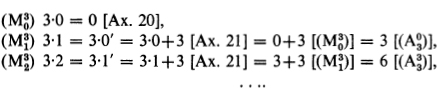
EXAMPLE 1. The following is a (formal) proof in N. Strictly speaking, the proof is the sequence of 17 formulas. In addition, numbers have been supplied at the left, and explanations at the right.

Thus (the reflexive law of equality) is a provable formula; or in symbols, (Here "" is not a formula, but a statement in our metamathematical shorthand that the formula is formally provable.)

Now we give informal proofs in the formats (A) and (B₂) (cf. §§ 13, 25) of the fact that (i.e. that a formal proof of exists).

1. true because the formula concerned is Axiom 16.

(A) 2. from 1 by substituting , for (Theorem 21 Corollary 2 (d) for empty).

3. true because is Axiom 18.

4 from 3 and 2 by two applications of ⊃-elim

Substituting for in Axiom 16,

(B₁) From this and Axiom 18 by ⊃-elims., .

Repeating in part some points made in Chapters I and II (especially §§ 10, 13, 25), formal proofs even of simple formulas tend to be long, as Example 1 illustrates. We are interested in what formulas there are formal proofs of, i.e. in what formulas are formally provable. We shall be satisfied to know whether formal proofs of these formulas exist, and we shall not ordinarily care about actually seeing such formal proofs when we have shown that they exist. Therefore we find it satisfactory to use informal proofs to show that the formal proofs exist, when it is easier to do so and when the informal proofs are by “finitary” methods (§ 36, §37).¹⁵³ If challenged to find the formal proofs we have demonstrated to exist, we are then able to supply them. Continuing in the manner illustrated, our methods for informally proving (in metamathematics) the existence of formal proofs (now in the system N) can be brought quite close to the methods of the ordinary mathematician in developing the elementary theory of the natural numbers. However, we must not forget that we are doing something somewhat different than he; i.e. we must not lose sight of the path by which our informal proofs can be converted into formal proofs in N.

We shall go a bit further in illustrating the beginnings of the development of number theory in N, by giving a few more metamathematical or informal proofs that certain formulas expressing theorems of elementary number theory have formal proofs in N.

From the reflexive property of equality (*100) and Axiom 16, we readily obtain the symmetric and transitive properties (*101) and (*102).¹⁵⁴ (If it isn’t obvious, refer to Theorem 29 in § 29.)

Having the reflexive, symmetric and transitive properties of equality, we can use chains of equalities analogously to chains of equivalences in § 5, except that we do not yet have the general replacement theorem (Theorem 30, analogous to Theorem 5) to use in justifying links of the chains. We use chains to simplify the presentation in the next example.

EXAMPLE 2. We show that (*104). (In the terminology of § 29, this is one of the two open equality axioms for +.) Preparatory to using ⊃-introd., assume (a) . Preparatory to applying Axiom Schema 13 (“mathematical induction”) with as the x, A(x), we need to deduce (from ) the two formulas and I. (Basis.) [Ax. 18 with substitution; this gives (cf. Example 1 (A) Step 2), whence by the symmetric property of equality ]. So (using the transitive property of equality, implicit in the chain method) . II. (INDUCTION STEP.) Preparatory to ⊃-introd., assume (b) Then [Ax. 19 with subst.] [using (b) and Ax. 17, with subst. and ⊃-elim.] [Ax. 19 with subst.]. By the planned ⊃-introd. (discharging the assumption (b)), Thence by ∀-introd. (since our remaining assumption (a) does not contain free), . III. By Ax. Sch. 13 with the results of I and II and &-introd. and ⊃-elim., . By ⊃-introd. (discharging (a)),

Next we can establish (the provability of) the other equality axiom for +, namely (*105), though this isn’t quite so easy (Exercise 38.2). The two for · can be shown to be provable similarly. Then we will have all the axioms of the predicate calculus with equality (§ 29) which go with the symbolism of N. So by Theorem 30 in § 29, we will have the replacement property of equality in general; so chains of equalities can be constructed using any replacements based on available equalities. (Before we had to be careful to use replacement steps only when we had special justification, as by Axiom 17 in II of Example 2.) Now (or earlier, after establishing just the equality axioms for +), we can prove the associative law for addition (*117; Exercise 38.3), etc.

The foregoing gives only enough of a beginning to convey an impression of how the development of number theory in N would go. A week or two of study would bring us quite far in this development.

By carrying such a development quite far, partly in a straightforward way as illustrated, and partly through investigations of a general nature, it can be said to be established that the system N is adequate for the usual elementary number theory such as occurs in standard texts (but not for analytic number theory, end § 36). By this we mean that, first, the predicates and propositions commonly used in informal elementary number theory can be expressed by formulas in N, and, second, for those propositions which are commonly proved as theorems in informal number theory, the formulas expressing them are formally provable in N (as illustrated by a few simple examples just now).

The first part calls for a little explanation. We have already seen that, although is not provided directly in the formal symbolism, a formula is so provided which under the (intended) interpretation expresses a<b. By introducing “<” as a symbol of abbreviation, we can thus express inequalities. That a divides b can be expressed by which we abbreviate “”. That a is a prime number can be expressed by , which we abbreviate “Pr()” . Euclid’s theorem that there are infinitely many primes can be expressed by . The provability of this formula is established in IM p. 192 *161, where it appears about 60 results later than our Exercise 38.3. (By no means all intervening results are used in its proof.)

Since 0, ′, +, · are the only function symbols in N, besides which variables are available, no function other than a polynomial can be expressed by a term of N. This is undoubtedly a limitation in the symbolism of N, but it can be circumvented. For what can be expressed informally using functions can in fact be paraphrased using predicates instead. Thus, say f(x_l , . . . , x_n ) is a number-theoretic function of n variables, and let F(x_l , . . . , x_n , y ) be the predicate of n+1 variables which is true for exactly those n+1-tuples (x_l , . . . , x_n , y) such that f(x_l , . . ., x_n) = y. We call F(x_l , . . . , x_n y) the representing predicate off(x_l, . . . , x_n) . What can be stated using f(x_l , . . . , x_n) can be paraphrased using F(x_l , . . . , x_n y) instead. For example, consider the function x! (where 0! = 1 and (x+1)! = 1 · 2 ·. . . . · (x+1) with x+1 factors). Let F(x, y) express x! = y, Take the proposition (x+1)! = x!(x+1) which is an (informal) theorem about the factorial function. This can be paraphrased in terms of the predicate F(x, y) e.g. thus:

Now it turns out that, although only polynomials can be expressed in N by means of terms, the representing predicates F(x_l,. . ., x_n, y) of a vastly greater class of functions can be expressed in N.¹⁵⁵

Furthermore, not only can the propositions using such functions be expressed indirectly by using their representing predicates, but all the reasoning that could be carried out with the functions can be paralleled too.¹⁵⁶

Thus it comes about that N is adequate for the usual elementary number theory despite its obvious shortage of function symbols.

One might ask: Would it not be better to remedy this deficiency by constructing another system with more function symbols ? One can do this, but for foundational questions it is often best to keep the system as simple in its structure as possible. In fact, the theory just cited allows us to use such systems richer in functions than N and construe all the results in terms of N.

Another question is whether we could still get the same results with even fewer function symbols in the symbolism. Specifically, could we omit as a formal symbol, and omit Axioms 20 and 21, and then get the effect of · in the same way that in N we get the effect of x ! etc. ? The answer is “No”.¹⁵⁷

So far, in the case of N, we have used Hilbert’s idea of studying the formal system from outside by “finitary” methods (in metamathematics) mainly in developing short cuts by which we prove metamathematically (informally) that various formulas are formally provable. Hilbert intended of course that metamathematics should concern itself also with general questions about the formal system, such as those as to its consistency and completeness. (We did deal with both of these for the propositional calculus in §§ 11, 12, and with consistency for the predicate calculus in § 23.)

Ackermann in 1924-5 thought he had proved metamathematically the consistency of N. But von Neumann in 1927 pointed out that Ackermann’s proof is limited to the subsystem of N in which the use of Axiom Schema 13 (the induction schema) is restricted to the case of an A(x) which does not contain any free occurrence of x in the scope of a quantifier, i.e. in the B of a part ∀yB or ∃yB; at the same time von Neumann gave another meta-mathematical consistency proof for that subsystem.

The failure of metamathematicians to establish the consistency of N in the next few years was illuminated in 1931 by results of Gödel, which we will present in a general setting in Chapter V (especially §§ 43 44). These results begin with an answer to the completeness question (in which we ask whether N suffices for all elementary number-theory, not just for what is usually developed).

In the following chapters, N can always refer to the particular formal system described in this section (which is the simplest way to read those chapters), and sometimes (when we so indicate) N can also refer more generally to any system with similar properties.

Exercises. 38.1. Translate Example 2 (as given in the format (B₁)) into statements using the symbol (in the format (B₃)), and check it in the latter format (cf. §§ 13,25).

38.2*. Show that

38.3. Assuming the result of Exercise 38.2, and using the general method of Example 2, show that .

38.4. Show that i.e. establish statements of formal provability corresponding to (A₀³), (A₁³), (A₂³) ,. . . .

38.5. Show that, using besides predicate calculus only Axioms 14 and 15: ....

* § 39.Some other formal systems. In this section, we give further examples [2]-[50] of formal systems (where [1] is the system N of §38).

We now describe [2] a system G, which formalizes the elementary theory of an unspecified “group” (explanation follows).

The formal symbols shall be

Variables are to be constructed as in § 38 for N. (The only difference in the formation rules between N .and G is that + ,·, ′ , 0 are replaced by · ^-1 , 1 .)

DEFINITION OF “TERM”. 1. 1 is a term. 2. The variables . . . are terms. 3-4. If r is a term, so are (r)·(s) and (r)^-1. 5. The only terms are those given by 1-4.

Given this definition of “term”, the definition of “formula” from “term” reads as in § 38.

Parentheses are omitted under the same conventions as there. Furthermore (as we could also have done in § 38), we shall abbreviate r·s (i.e. (r).(s)) as “rs” (omitting the dot).

As postulates, we take those of the predicate calculus, with the present notions of “term” and “formula” (§§ 21,28); just as for N, the r for the ∀-schema and the ∃-schema can be any term free for x in A(x). In addition, there shall be the following six particular axioms:

El. . . .

Gl. (Associative law.)

G2. (Right identity.)

G3. (Right inverse of .)

We do not intend a single interpretation of this formal system G, as we did of N. The system G may be interpreted by any “group” G, as we shall explain and illustrate in a moment. For any choice of a “group” G, the terms are interpreted as naming members (specified or unspecified) of G (or more precisely of G₀, below).

Axioms E1-E3 give what we need to postulate of the properties of equality (identity).¹⁵⁸

The axioms G1-G3 for groups will be familiar to many students. A group G is briefly any “system” of objects which “satisfies” these three axioms (with the variables in the generality interpretation §§ 20,38, and with = expressing “identity” or “equality”§ 29).

That is, a group G consists of a nonempty set G₀, a 2-place function a.b with arguments and values in G₀, a 1-place function a^-1 with arguments and values in G₀, and a member of G₀ (or 0-place function) 1, such that the closures of G1-G3 are all t in our model theory of the predicate calculus with equality § 29 when G₀ is the domain and a·b, a^-1, 1 are the values of · , ^-1, l. ¹⁵⁹

To give only a few particular interpretations, G can be (1) the positive rational numbers with ·, ^-1, 1 having their usual meanings. (The student should have no trouble verifying that G1-G3 are satisfied by each of our interpretations.) Alternatively, G can be (2) the rational numbers except 0, (3) the positive real numbers, (4) the real numbers except 0, or (5) the complex numbers except 0, with ·, ^-1, 1 in their usual meanings. Still again, G can be (6) all the integers, (7) all the rational numbers, (8) all the real numbers, or (9) all the complex numbers, with · , ^-1, 1 meaning a+b , — a , 0, respectively.

As an interpretation not by a number system, G can be (10) or (11) all the possible rotations of a square within its plane, or through three-dimensional space, into itself. That is, we are to rotate the square so that after the rotation it occupies the same portion of space as before, but the original corners may be in new positions; e.g. if the original square is ABCD, then after the rotation A may be where D formerly was, B where A formerly was, etc. Also, turning the square by —90° or 270° or 630° about an axis perpendicular to its center is considered the same rotation; so “rotation” really means “result of rotation”. Now · is interpreted to mean (the result of) the rotation a followed by the rotation b. The further details are left to the student (Exercise 39.1).

Similarly, G can be (12) or (13) all the possible rotations of a circle into itself, or (14) all the possible rotations in 3-dimensional space of a cube into itself, or (15) of a sphere into itself.

Now we demonstrate (informally) the (formal) provability of a number of formulas (writing “T” for “theorem”). Proofs not given are exercises. As was remarked for N in § 38, the direct rules of the predicate calculus, and also all of the introduction and elimination rules of THEOREMS 13 and 21, hold good for G .

T1. (Reflexive property of equality.)

PROOF (in the format (B₁)). By substituting for in Axiom E1 , . Thence using G2 and ⊃-elim. twice, . The next two follow as did *101 and *102 in § 38.

T2. (Symmetric property of equality.)

T3. (Transitive property of equality.)

Having now the reflexive, symmetric and transitive properties of equality, we can use chains of equalities (though without unrestricted replacement yet; cf. § 38).

T4. (Left inverse of , the same as our right one.)

PROOF. (by a chain of equalities) . [G2 (and substitution)] = .

T5. . (Left identity, the same as our right one.)

PROOF. .

T6. . (Uniqueness of right identity.)

PROOF. Assume for ⊃-introd., . Now x = 1 x [T5] = [by the assumption with E3] = 1 [T4] .

T7. . (Uniqueness of left identity.)

T8. . (Uniqueness of right inverse of .)

PROOF. Assume . Now = [by the assumption .

T9. (Uniqueness of left inverse of .)

T10. . (Equality axiom for ^-1.)

PROOF. Assume = Then [by the assumption = with E2] = 1 [G3]. So by T8, .

Now we have the equality axioms for all our symbols (in Tl, El, E2, E3, T10). So hereafter we can replace on the basis of equalities without restriction (Theorem 30 § 29).

Furthermore, having now both the replacement property of equality and the associative law Gl, we shall hereafter write (rs)t and r(st) as “rst”, so applications of Gl become tacit.

T11. . (Right cancellation.)

PROOF. Assume . Then .

T12. . (Left cancellation.)

T13. . (Inverse of inverse of .)

PROOF. .

T14. . (Inverse of a product.)

HINT FOR PROOF: Use T8.

Next we describe [3] a simpler formal system Gp of group theory. For this, we omit the function symbol ^-1 and the individual symbol 1 from the list of formal symbols, correspondingly simplifying the definition of “term” and thence of “formula”. We replace G2 and G3 by the following two axioms.

Gp2. .(Existence of right quotient.)

Gp3. .(Existence of left quotient.)

That is, the postulates are those of the predicate calculus and the six axioms E1-E3, Gl, Gp2, Gp3. This corresponds to defining a group G as a system satisfying the axioms Gl, Gp2, Gp3.

Thl. . (Reflexive property of equality.)

PROOF. Substituting for in Gp2, . Preparatory to ∃-elim., assume . Substituting into Using ⊃-elim. twice, . Now we complete the ∃-elim.

Th2. . (Symmetric property of equality.)

Th3. . (Transitive property of equality.)

Th4. . (Existence of right identity.)

PROOF (using E2, E3, Gl tacitly). Assume for ∃-elim. from formulas obtained from Gp2 and Gp3 by changes of bound variables (*74 § 24) and substitutions: , (The x of each ∃-elim. will be the underlined variable.) Now , so by . Also , so by . By . Now we complete five ∃-elims., discharging successively the assumptions (6)-(2), use ∀- and ∃-introd. to get , and finally discharge (1) by the sixth ∃-elim.

Now we shall sketch why Gp formalizes essentially the same theory as G. Since the axioms of Gp (unlike those of G) are symmetric with respect to · , without further work we can write down Th5.

Th5. . (Existence of left identity.)

Th6. . (Equality of right and left identity.)

Th7. . (Uniqueness of right identity.)

(Hint: use Th5, Th6.) For the abbreviation “∃!xA(x)”, cf. § 29.

Th8. abbreviated

. (Unique existence of right identity.)

(HINT: use Th4, Th7.) The formula expresses the representing predicate 1=i of the right identity 1 as a 0-place function (cf. end§ 38), and the provable formula of Th8 says that is a representing predicate. Now the conditions for the application of the eliminability theorem cited in Footnote 156 § 38 are fulfilled. By that theorem, we can add the individual symbol 1 to the symbolism of Gp, and the formula , or with the same effect G2, to its axioms, to obtain a system Gp₁ with the following properties. In Gp₁, exactly the same formulas not containing 1 are provable as in Gp. Each provable formula of Gp₁ containing 1 can be paraphrased, as illustrated at the end of § 38, by a provable formula of Gp.

Now we develop similarly the theory of the inverse a^-1 inGp₁.

Th₁14. (Unique existence of right inverse of .)

The formula =1 expresses the representing predicate a^-1 = b of a^-1. By a second application of eliminability, we can add to Gp₁ the function symbol ^-1 and the axiom G3, obtaining a system Gp₂. But by Exercise 39.2, Gp2 and Gp3 are redundant in Gp₂ (being provable in its "subsystem" G), and thus they can be omitted as axioms of Gp₂, doing which gives G.

We conclude hence that in G exactly the same formulas not containing ^-1 or 1 are provable as in Gp, while the provable formulas of G containing ^-1 or 1 can all be paraphrased by provable formulas of Gp. Thus G is in the same relation to Gp as the richer systems of number theory alluded to at the end of § 38 are to the system N.

Our examples of groups except (11), (13), (14) and (15) satisfy an additional axiom:

G4. . (Commutative law.)

Such groups are called commutative or Abelian. Formal systems [4] AG and [5] AGp for Abelian groups are obtained by adding G4 to the postulates of G and Gp, respectively.

To see that (11) does not satisfy G4, say the square is in a horizontal plane with edges running north and east. Let a be a clockwise rotation of 90° (as seen from above) about a vertical axis through the center of the square, and b be a rotation of 180° about a horizontal axis running east through the center. Then the results ab and ba of performing these two rotations in different orders are different, as the student may verify. Similarly with (13), (14) and (15).

Our groups are infinite, i.e. have infinitely many elements in the set G₀, except (10), (11) and (14), which are finite. —

As we remarked in § 37, we get specific formal systems of propositional and predicate calculus by supplying suitable definitions of “atom”, and of “ion” or of “ion” and “meson”.

We begin with [6] the pure propositional calculus P_p. For this, we introduce a new species of formal symbols . . . (script capitals), called proposition letters.¹⁶⁰ The problem of what to do after the twenty-sixth letter can be handled as we did for number theory N, by using a formal symbol _| to manufacture additional proposition letters. Most treatments simply assume there is a potentially infinite list of proposition letters (and likewise of variables for number theory). The other formal symbols are ~, ⊃ , &, V, ¬ and parentheses. “Formulas” are defined as in § 1 with the proposition letters now being the atoms (and with parentheses handled as in § 38, or in some other suitably explicit manner). If we have to talk about both these formulas and those of formal number theory N in the same context, the two kinds may be distinguished as proposition letter formulas and number-theoretic formulas. The postulates, of course, are Axiom Schemata la-10b and the ⊃-rule.

Similarly, we obtain [7] the pure predicate calculus Pd by using as the ions We call these predicate letters.¹" Infinitely many of them are to be available with each number n ≥ 0 of open places; we may get these either by assuming an infinity of script capital letters as formal symbols, or by using _| to manufacture others after the twenty-six the printer really has. The other formal symbols are ~ , ⊃ , &, V , ¬, ∀, ∃, variables . . . (infinitely many, or twenty-six with _| to form others), the comma and parentheses. Thence “formula”, or more specifically “predicate letter formula”, is defined as in § 16 with the predicate letters now being the ions (and an explicit treatment of parentheses). The postulates are Axiom Schemata la-10b, the ∀- and ∃-schema (as originally stated in § 21 with just variables as the terms), and the ⊃-, ∀- and ∃-rule.

By adding to the predicate letters as ions also (—) = (—) (read “ — equals — ”), and to the postulates the open equality axioms for = and for each predicate letter with n > 0 open places, we obtain [8] the pure predicate calculus with equality Pd =.

Now let us take as mesons (§ 28) the expressions , . . . , , . . . , which we call function letters.¹⁶⁰ Here .. . are lower case script letters from the middle of the alphabet, which are to be removed from use as variables. (We may either assume an infinite supply of these letters as well as of the letters for variables, or reserve finitely many for each use and manufacture others using _|.) With the rest of the formation rules and the postulates taken as in § 28 or § 29, we thence obtain [9] the pure predicate calculus with functions Pdf and [10] the pure predicate calculus with functions and equality Pdf=.

In these pure systems, the atoms or ions (or also mesons) are provided completely generally, without reference to any particular application of logic.

But also we can have formal systems of propositional calculus and of predicate calculus without or with equality by using the formation rules of a more complicated or more special system. Thus using “formula” as for Pd, Pd=, Pdf, Pdf=, N, G or Gp with just the postulates of the propositional calculus (Axiom Schemata 1a-10b and the ⊃-rule), we get respective systems [11]-[17] of propositional calculus. Using “formula” (or “term” and “formula”) as for Pd=, Pdf=, N, G or Gp with the postulates of the predicate calculus Pd or Pdf, we get systems [l8]-[22] of predicate calculus. Using “term” and “formula” as for N, G or Gp with the postulates of the predicate calculus with equality Pdf =, we get systems [23]-[25] of that. The treatments of propositional calculus, of predicate calculus and of predicate calculus with equality in Part I were framed to apply to any of these systems and others.

The systems of logic [15]—[17], [20]-[22] and [23]-[25] using the formation rules of N, G or Gp are examples of applied systems of logic, as their formation rules are chosen with a view to the application of the system to a more or less specific subject matter. Thus, an applied predicate calculus (illustrated by the “number-theoretic predicate calculus” [20]) has a list of s ≥ 1 predicate symbols or possibly other ions P_l,. . .,P_s (each with a specified number p_i ≥ 0 of open places) and a list of t ≥ 0 function symbols or possibly other mesons f_l,. . . ,f_t (each with a specified number q_i > 0 of open places).¹⁶¹ Thence “term” (= “variable” if t = 0) and “formula” are defined as above (§ 16, or for t > 0 §28, but with an explicit treatment of parentheses § 38). For the number-theoretic predicate calculus, P₁,..., P_s is (—) = (—) simply (s = 1, p₁ = 2), and f₁,. . ., f_t is (—)+(—) , (—) · (—) , (—)′ , 0 (t = 4, q_i= q₂ = 2, q₃ = 1, q₄ = 0). In an applied predicate calculus, the predicate and function symbols or other notations have one or more “intended” or “standard” interpretations. (Of course, these can play no part in the metamathematics.) Applied systems of logic give a formalization of the logic to be used in a particular subject, e.g. number theory, directly in the formalized language of that subject. This corresponds closely to how the mathematician or layman uses logic.

By using in place of Axiom Schema 8 the intuitionistic Axiom Schema 8¹, we obtain intuitionistic systems [26]-[50] corresponding to the classical systems [l]-[25]. (Cf. ends §§ 12,25.)

Exercises. 39.1. For the group of rotations of a square into itself, show that there are 4 or 8 elements according as the square must remain in its plane or not during the motion. What are the interpretations of 1 and ^-1 for this group ?

39.2. Using T1-T5, show that and .

39.3. Prove T7, T9, T12, T14.

39.4. The part of the proof of Th4 ending with (9) demonstrates that (1), (2), (3), (4), (5), (6) (9). Show explicitly the rest of the steps (after (9)) in the format (B₃), and verify the correctness of each ∃-elim. and the ∀-introd.

39.5. Prove Th6-Th8 and Th₁-Th₁.

¹²¹ That an infinite collection can be put into 1-1 correspondence with a proper part of itself was noticed a number of times before Gallileo. Steele (in his historical introduction to his 1950 translation of Bolzano 1851, who noted the same) cites Plutarch (467-125? A.D.) and Proclus (412-485 A.D.). Thomas 1958 cites Adam of Balsham (Parvipon- tanus) 1132, and Pierre Duhem “Le systeme du monde” 1954 ed. vol. 7 p. 123 cites Robert Holkot (d. 1349). Julius R. Weinberg supplied these references and also “Centriloquium Theologicum”, Conclusio 17 (erroneously attributed to William Ockham (d. 1349?)).

¹²² Some authors use “natural numbers” as a synonym for “positive integers” 1, 2, 3,. . . , obliging one to use the more cumbersome name “nonnegative integers” for 0, 1, 2,. . . . Besides, in this age, we should accept 0 on the same footing with 1 2, 3,. . .

¹²³ This is surely the more intuitive definition of finiteness of a set. But the property of the set of the positive integers noted in Gallileo’s “paradox” is characteristic of infinite sets. So, as Peirce 1885 and Dedekind 1888 proposed, a finite set can be defined alternatively as a set which cannot be put into 1-1 correspondence with a proper part of itself. Cf. IM pp. 13, 14 (after reading § 34 below).

¹²⁴ (1, 2, 3), (2, 1, 3), (2,1,1,3) are different finite sequences; but the sets with members shown in curly brackets {1, 2, 3}, {2, 1, 3}, {2,1,1, 3} are the same.

¹²⁵ We have formulas (i.e. finite names) for these five functions. But also functions are to be included whose successive values are determined by laws not corresponding to ordinarily used names, and even functions whose successive values are picked “irregularly” or in a “random” manner.

¹²⁶ A proof (to follow § 34) is given in IM pp. 16, 17.

¹²⁷ Cantor also developed a theory of point sets, much of which has now become familiar in the form of point set topology.

¹²⁸ Cantor 1895-7 is quite readable, and has been translated into English (cf. our bibliography). Fraenkel 1961 gives an excellent and very full account. A concise treatment is in Bachmann 1955.

¹²⁹ We are repeating a little from § 26 above to make the present chapter largely self-contained.^89,^91,^92,

¹³⁰ A treatment is given in IM pp. 12, 13 with Example 1 § 7 p. 22.

¹³¹ For some historical details and references, see Weyl 1949 p. 228 Footnote 2.

¹³² The pages in the 1953 edition are 21, 22, 24, 28, 42, 97, 123.

¹³³ Godel 1947 provides a very readable exposition.

¹³⁴ It reads: If two straight lines in a plane meet another straight line in the plane so that the sum of the interior angles on the same side of the latter straight line is less than two right angles, then the two straight lines will meet on that side of the latter straight line.

¹³⁵ This kind of treatment of axiomatic systems is well presented in J. W. Young 1911. Several of the topics mentioned briefly now will be elaborated below: independence proofs in § 57; categoricity in § 53; consistency proofs by interpretation in § 52.

¹³⁶ Hilbert and Bernays 1934 pp. 15-17; quoted on IM pp. 54-55.

¹³⁷ We gave a little fuller sketch in IM § 13. Excellent introductions are in Heyting 1934, 1955 and 1956. Kleene and Vesley 1965 is intended for readers familiar with IM Chapters I-XII (or as a minimum IV-VIII) or the equivalent.

¹³⁸ See Weyl 1949 pp. 50-62.

¹³⁹ W. W. Rouse Ball 1892 (pp. 80-81 in the 11th ed. 1939). Reproduced in J. W. Young 1911 pp. 143-145.

¹⁴⁰ If that informal or semiformal mathematics is ambiguous (like abstract group theory), admitting different interpretations, then we can use “interpretation” here in either the singular or the plural, depending on where the focus of our attention is, on the semiformal mathematics as the mathematician works with it while developing it, or on its interpretations in turn.

¹⁴¹ In our “proof theory” in Part I we did use only finitary methods, though we didn’t say so. In “model theory”, the methods are not restricted to be finitary. In modern “model theory”, we would likewise work with a completely symbolic language. Just as Hilbert is responsible for “proof theory” in its present refinement, Tarski 1933, 1935 etc. is the originator of much of modern model theory. Carnap 1935 did some work similar to Tarski 1933. Sometimes proof theory is called “syntax” and model theory “semantics”. For a full bibliography of model theory, see Addison, Henkin and Tarski 1965.

¹⁴² At the same time, as will appear in § 38, we need to be a little more explicit about how parentheses are used.

¹⁴³ Inversely, computers may be applied in metamathematics to seeking proofs of theorems, or to checking proposed proofs, etc.¹⁵³

¹⁴⁴ If it is more convenient to use “a₁” , “a₂” , “a₃”, . . . than “a_|”,“a_||” , “a_|||” , . . . we can do so in practice by regarding the former as metamathematical abbreviations for the latter.

¹⁴⁵ A point arises here with respect to all the formal symbols including the variables, which was discussed in § 1 Footnote 6 for ~, ⊃, &, V, ¬ when they are symbols of the object language (as here). To get names of the formal symbols in the syntax language, we simply use specimens of those symbols as names for themselves (“autonymously”).

¹⁴⁶ It is important to remember that the formulas of a formal system are not just any formulas of informal mathematics, or any finite sequences of (occurrences of) the formal symbols of the system; but they are just those finite sequences of the formal symbols which are formed in accordance with the rules defining “formula” (here the nine rules just listed).

To emphasize this, many authors call them “well-formed formulas” or “wfTs”. (To be consistent, if we did so here, we ought to say also “well-formed terms” or “wfts”, and “well-formed proofs” or “wfps”.) We find “well-formed formulas” and “wffs” a little aneuphonious (unwell-sounding). So we prefer, after the well-taken point has been well-emphasized, to say simply “formulas” (following Hilbert and Bernays 1934, 1939). For the infrequently needed arbitrary finite sequences of formal symbols, we have the longer name “formal expressions”.

¹⁴⁷ See IM pp. 23-24, 73-74.

¹⁴⁸ Most of the next remarks (down through (A) and (B)) apply similarly to any formal system consisting of the predicate calculus, or the predicate calculus with equality, plus nonlogical axioms. This includes the predicate calculus with equality itself as based on the predicate calculus without equality (§ 29). For systems based on the predicate calculus with equality, the “nonlogical axioms” are those added to the axioms of the predicate calculus with equality.

¹⁴⁹ We rely on the context to make it clear when 0, ’,+,*,· = are being used as formal symbols and ≠, <, >, 1, 2, 3, . . . in abbreviating formal expressions, and when they are being used informally.

¹⁵⁰ A closed formula is called a sentence by Tarski (in the Eng. tr. of 1933, in Tarski, Mostowski and Robinson 1953, etc.). We are using “sentence” simply for the linguistic objects (declarative sentences) in the informal language which are formal ized by formulas, open or closed.

¹⁵¹ A proof of B in N using as nonlogical axioms only A_i,..., A_m is not in general a deduction of B from A₁ .. ., A_m in the predicate calculus with all variables held con stant. For in the latter (§21), we are restricted in using the V-rule and the 3-rule below the first use of A₁,.. ., A_m to variables not occurring free in Ai,..., A_TO. In a proof in N, where A₁ .. ., A_m count as axioms rather than as assumption formulas with their variables held constant, this restriction is lifted. Hence the V’s are necessary in (A).

¹⁵² Peano dealt instead with the positive integers. A quite full explanation of these axioms is in IM §§ 6, 7 (and in § 8, which overlaps the present§ 36). That explanation is not essential to the present survey. The role of the fifth Peano axiom (Axiom Schema 13) is illustrated in Example 2 below; of the third and fourth, in Exercise 38.5.

¹⁵³ If computing machines are to be applied to seek or check proofs, a further step is appropriate. Some selection of the quicker and easier methods to which our metamathematical investigations have led us, or (for seeking proofs) possibly of other methods tailored to the machines strengths and weaknesses, should be stereotyped as a new formal system in which the computer is to make its searches or perform its checks. Here we are not referring just to formal number theory, but also to the predicate calculus and other systems obtained by adding mathematical axioms to it. Cf. Wang 1960, Davis and Putnam 1960, J. A. Robinson 1963, 1965.

¹⁵⁴ We give parenthetically the numbers with which these results appear in IM Chapter VIII.

¹⁵⁵ This is a consequence of work of Godel 1931 and Kleene 1936 (cf. IM §§ 48, 49,57, or specifically Theorem VII (b) p. 285).

¹⁵⁶ The basic step is the elimination of “proper definite descriptions” (§ 31), using a theorem of Hilbert and Bernays 1934 (cf. pp. 422-457 and 460 ff.). There is a treatment in IM pp. 407-419. The theorem gives directly conditions under which the effect of f(x₁ ..., x_n) can be secured in a system in which we have F(x_l, ...,x_n, y). It is a proof- theoretic version of Theorem 32 § 31.

¹⁵⁷ This follows by combining a result of Presburger 1930 and Theorem IV in § 43 below. (Cf. IM pp. 204, 407.)

¹⁵⁸ Alternatively, we could have started from the predicate calculus with equality (§ 29), thus automatically postulating five open equality axioms (or their equivalent),¹⁰⁸and have added just the three axioms G1-G3.

¹⁵⁹ Textbooks on (informal) group theory are e.g. Marshall Hall 1959 and Rotman 1965.

The symbols “·;”, “^-1”, “1” are often chosen differently. Particularly, “·” is often written as “ ° ” to suggest a variety of interpretations, in some of which ° will not be the usual multiplication, and “1” as “i” (the “identity”).

“Group theory” includes nonelementary parts (e.g. subgroups, isomorphism, representations), not formalized in G.

¹⁶⁰ In systems having particular axioms and a postulated substitution rule (in contrast to axiom schemata and a derived substitution rule),⁸⁶ . . . are called proposition variables. Cf. § 9 just after Example 4.

In similar treatments of the predicate calculus, what we call “predicate letters” are called “predicate variables” (or some by authors “functional variables”);⁵¹ and similarly with functions, our “function letters” becoming “function variables”.

¹⁶¹ This covers most uses of the term “applied predicate calculus”. One can also consider systems with infinitely many predicate or function symbols, and systems with a mixture of these notations and those of the pure systems.