CHAPTER II

THE PREDICATE CALCULUS

§16. Linguistic considerations: formulas, free and bound occurrences of variables. In the propositional calculus, we studied those logical relationships which depend on how some propositions are composed from other propositions by operations (expressed by the symbols ∼ , ⊃, &, V, ¬) in which the latter propositions enter as unanalyzed wholes. In the predicate calculus, we carry the analysis a step deeper to take into account also what in grammar is called “subject-predicate structure”, and we use two further operations, ∀ (“for all”) and ∃ (“for some” or “there exists”) which depend on that structure. (The predicate calculus includes the propositional calculus.)

Consider the proposition (expressed by the sentence) “Socrates is a man”. The part of this proposition (expressed by) “— is a man” or “x is a man” is a predicate; “Socrates” is a subject. Read “x is a man”, using the mathematical notation of a variable, the predicate is seen to be a propositional function, i.e. for each value of the (independent) variable “x”, it becomes (or takes as value) a proposition, true for example when x is Socrates, false in Greek mythology when x is Chiron, and in the Kleene household when x is Fleck. To take another example, “John loves Jane” is a proposition, which can be thought of as a value of any one of three propositional functions, “x loves Jane”, “John loves y” and “x loves y” In grammar, “x loves Jane” is a predicate, but not “John loves y” or “x loves y”; and a value of “x” is a subject, of“y” an object. Mathematically, these distinctions are unimportant. We shall simply adopt the term predicate as short for the more cumbersome propositional function P(x₁, . . . , x_n), for any number n ≥ 0 of (independent) variables ;⁵⁰ and the term object or individual for a value of any one of the variables. For n = 0, we have & proposition as a special case of a predicate; for n = 1 a property; for n = 2, a (binary) relation; for n = 3, a ternary relation; etc.

This explains the name predicate calculus for the logic of propositional functions. A fully descriptive (but cumbersome) name is calculus of propositional functions .⁵¹

The notation“x is a man” is a bit more concise than “— is a man”. The advantage of variables over blanks to show the “open places” in a predicate is increasingly apparent in examples like “—₁ loves —₂“, “—₁ loves —₁” (synonymous with “— loves himself”), and “—₁ is father of — ₂, or —₁ is mother of —₂” (synonymous with “—₁ is a parent of —₂”).

Such expressions as“—₁ loves —₂” ^or“x” loves“y” are not used directly in ordinary language.⁵² To relate them to ordinary language, we may begin by regarding the blanks or variables which we have introduced as“place holders” for words naming objects. Of course, the words to be supplied do not need to be proper nouns, like “John” and “Jane”. We can have, for example: (a₁) “Somebody loves Jane”, (a₂) “There is someone who loves Jane”, (b) “Nobody loves Jane”, (c) “Everybody loves Jane”, (d) “Everybody loves someone”, (e) “Someone is loved by everybody”, (f) “Everybody loves himself”, (g) “There is no one who does not love himself”. Using “L(x, y)” as short for “x loves y” and supposing for the moment that “bodies” or persons are the range of the variables “x” and “y”, these can be written using ∀ and ∃, thus: (a′) ∃xL(x, Jane), (b′) ∼∃xL(x, Jane), (c′) ∀xL(x, Jane), (d′) ∀x∃yL(x, y), (e′)∃y∀xL(x, y) (f′) ∀xL(x, x), (g′) . In this symbolism we have formed sentences expressing propositions, without displacing or completely displacing the variables "x" and“y". Note particularly that in (a′) as expressing (a₂) (which is synonymous with (a₁)), “someone” and “who” are each represented by an (occurrence of) “x”; similarly, three different words of (g) are each represented in (g′) by an “x”.

Here, rather than thinking of variables as simply (or always) “place ”, they may be thought of as a stock of names (nouns or pronouns), which are available to us to name various objects. What objects are named may depend on how they are incorporated into sentences, or on the context in which those sentences appear.

The use of variables is thus not basically so very different from constructions that are used in ordinary language.“Somebody” and“everybody” serve as names for unspecified persons; and even the proper name“Jane” isn’t specific, unless we have explained that we mean Jane Austen, or Jane Grey, or Jane Addams, or Jane who lives down the street. The legal“John Doe” is the equivalent of a variable (ranging over men) whose value is being left unspecified.

In the propositional calculus we studied logical relationships between propositions without taking into account what propositions are expressed by the prime formulas. This comes to the same thing as saying that, for the logical relationships we dealt with there, the propositions expressed by “P”, “Q”, “R”, . . . could be any propositions. Likewise, here we shall not identify the objects or individuals which may constitute values of the variables. To keep the symbolism as simple as we can in this chapter, we shall also not assume any other list of names for individuals to be provided than the one list of variables. So, if we wish to symbolize (a₁) “Somebody loves Jane”, we shall have to write e.g. ∃xL(x, y) (or ∃xL(x, j)) and agree that “y” (or “j”) is a name for the person Jane. This is not too great a sacrifice here, since we shall only be concerned in this chapter with general logical relationships, in which the special charms of Jane won’t figure (or at least only to the extent they are enumerated, and the relationships will then apply to any other lady possessing all those same charms). Later (§ 28), some symbols different from variables may be provided as names for particular individuals.

We return to the matter of notation for predicates. To take a mathematical example now,“x<y” can be used to name a predicate. Then when (x, y) become or take as values (2, 7) or (5, 100), x < y becomes or takes as value a true proposition. When (x, y) become (7, 7) or (100, 5), x < y becomes a false proposition. Now if we say (h)“For every (real) number x, there exists a number y such that x < y” (or in our new symbolism, (h′) ∀x∃yx < y) ,the “x < y” as part of (h) or (h′) is not being used to name a predicate, but to say something about two numbers, the first an arbitrary (i.e. completely unspecified) number named by “x”, and the second a suitably chosen number named “y” (the choice depending on the number named “x”). This example illustrates that it is necessary (but we think, easy) to distinguish between the use of an expression like “x < y” to name a predicate, and its use to express a proposition which is the value of that predicate when “x”, “y” are being thought of as naming objects.⁵³.only necessary to keep clearly in mind that a predicate P(x, y) is not a proposition, but a correspondence (or correlation) by which, from the various choices of pairs of objects as values of “x”, “y”, respective propositions arise.

So long as“x < y” is used just to name a predicate, it is quite satisfactory to think of“x” and“y” as place holders, not (or not yet) naming anything. But mathematicians, without changing“x” and“y” to anything else, then often go over to thinking of“x” and“y” as naming objects; so by a transformation in interpretation, the expression“x <y” for a predicate becomes an expression for a proposition, as we have illustrated. It is the ease with which this transformation can be made that accounts in part for the popularity of variables as a notational device.

The predicate (= propositional function) named by“x < y” can also be named simply “<”. Similarly, the function named “sinx” can be named simply“sin” or “sine”; but there is no commonly used name for the function x² + 3x + 1 that does not contain “x” (or some other variable instead). The vast majority of predicates we shall wish to name will not have commonly used names without variables.

A notation for a predicate using variables we may call a name form for the predicate. The variables used as part of such a notation constitute the name form variables in that notation, and have the predicate interpretation or the name form interpretation. We postpone further discussion of the use of variables in expressing propositions.

We began our study of the propositional calculus in § 1 by assuming that we are dealing with one or another object language, and that in this object language there are some (declarative) sentences (expressing propositions) which are to retain their identity throughout any particular investigation in the propositional calculus but are not to be analyzed in the investigation.

Now, to get started on our study of predicate logic, we need to assume that the object language contains some expressions or linguistic constructions for predicates (of given numbers of variables), which expressions shall retain their identity throughout any particular investigation in the predicate calculus but shall not be analyzed. These expressions we call prime predicate expressions or ions, and we denote them by “P”, “P(—)”, “P(—,—)”, “P(—, —,—)”, . . . , “Q”, “Q(—)”, “Q(—, —)”, “Q(—, —, —)”, . . . , “R”, . . . , also using subscripts when convenient.⁵⁴ Each capital Roman letter from the latter part of the alphabet will be used as a name for a different n-place prime predicate expression or ion for each number n ≥ 0 of variables; thus P, P(—), P(—, —), P(—, —, —) are four different ions (expressing respectively a 0-, 1-, 2- and 3-place predicate), and Q, Q(—), Q(—, —), Q(—, —, —) are four other ions. By including n = 0, we allow P, Q, R, . . . , expressing propositions, as in the propositional calculus; i.e. any atoms we had there which we do not now analyze further are allowed as the n = 0 case of n-place ions.

As in § 1, we are remaining silent here about what exactly the underlying object language is, both because we do not wish to be drawn into details about it now, and because we wish to leave the way open to various applications. The object language may be a symbolic language constructed by logicians using logical symbols, and perhaps also mathematical symbols; or it may be a suitably restricted and regulated part of English or some other natural language, without or with mathematical symbols added. Now we need to operate with variables; and we now agree to use the small Roman letters “a”, “b”, “c”, . . . , “x”, “y”, “z”, “a₁” , “a₂”, “a₃”, . . . , “x₁”, “x₂”, “x₃”, . . . as names for variables (or their equivalent as in (a₁)-(g) above) in the object language. Our convention here is that distinct small Roman letters will be names for distinct variables (or their equivalent) in the object language, except when we say they need not be distinct.⁵⁵

Sometimes it will be more convenient to consider the predicates expressed by the ions (with blanks as place holders) as named by expressions with variables (as above we had a choice between“— loves —₂” and “x loves y”). We call P(x, y, z), P(y, z, x), P(u, v, w), etc. different name forms for the same 3-place prime predicate expression or ion P(—, —, —); the variables x, y, z or y, z, x or u, v, w are the name form variables in these name forms, and they are to be distinct (as in the three examples). We also call P(x, y, z), P(y, z, x), P(u, v, w) prime predicate expressions (or ions) with attached (name form) variables. In a particular logical analysis, one name form for a given ion is the most we will need; however we may need to choose the name form variables in it to avoid conflict with variables already being used in other ways (e.g. in Exercise 19.1 below). We do not allow P(x, x, y), P(x, y, x) etc. as name forms for a 2-place prime predicate expression; for these are not prime, but exhibit that the predicate named arises by identifying two of the variables of a 3-place predicate expressed by the ion P(—, —, —). Because in a 3-place prime predicate expression we exclude considering any further structure (otherwise it wouldn't be prime for us), the blanks in P(—, —, —) are to be filled independently, so we don’t need subscripts thus: P(—₁ —₂> —3)- Similarly, as a prime predicate expression,“— loves —” must be “—₁ loves —₂”; and “— < —” (or simply “<”)⁵⁶ must be “—₁ < —₂”.

Now we are ready to describe a class of sentences assumed to exist in the object language called formulas, just as we were in § 1 after introducing the atoms there. But here we are starting further down in the structure of the object language (or assuming the object language has more than the minimum structure assumed there); i.e. we must now start with the ions.

For each n-place ion P(—,. . ., —) and each choice of variables r_l9.. ., r_w not necessarily distinct, P(r_1?. . . , r_n) shall be a. prime formula or atom. For example, from the ion P(—, —, —), we obtain as atoms P(x, y, z), P(y, z, x), P(u, v, w), P(x, x, y), P(x, y, x), P(u, u, u), etc. From the ion P, we get just P as atom. From Q(—) we get Q(x), Q(y), Q(u), etc. (With n = 0, the atoms of the propositional calculus are again atoms here. With n > 1, the atoms are a more extensive class than the name forms of ions, since in the atoms the variables replacing the blanks need not be distinct.)⁵⁷

The formulas shall comprise exactly the prime formulas or atoms, and the additional formulas (composite formulas or molecules) constructive from atoms by repeated introductions of the logical symbols ∼, ⊃, &, ∨, , ∀, ∃, thus. If A and B are any formulas (either prime formulas, or composite formulas already constructed), then A ∼ B, A ⊃B, A & B, A ∨ B and A are (composite) formulas. If A is any formula, and x is any variable, then ∀xA (read “for all x, A”) and ∃xA (read “for some x, A” or “(there) exists (an) x (such that) A”) are (composite) formulas.

∀x is called a universal quantifier, and ∃x an existential quantifier. The quantifiers act as unary operators in building formulas, and with our other unary operator are ranked last under the convention for omitting parentheses. Thus,“xA ⊃ B” means (∀xA) ⊃ B, not ∀x(A ⊃ B).⁵⁸

So that there will be no ambiguity as to what the atoms are, we stipulate that none of them be of any of the seven forms A∼B, A ⊃ B, A & B, A ∨B, ¬A, ∀xA, ∃xA which the molecules have. Also each atom shall come unambiguously from just one ion. In brief, the internal structure of the ions (whatever it may be) shall be such that it cannot get mixed up with what is added in building formulas and shown explicitly in our symbolism for formulas.

For example, “— is a man”, “— loves —”, “— = —”, “— < —”,“—+—= —”, “2 · 2 = 4” could be ions (with 1, 2, 2, 2, 3, 0 places,respectively). Then “x is a man”, “y is a man”, “x loves y” “x loves x”, “x = y”, “y” = “y” ,“x + y = z”, “x + x = y”, “2 · 2 = 4”, etc. will be atoms; and these can include “Socrates is a man” and “Chiron is a man”, or “John loves Jane”, if we interpret “x” and “y” as names for Socrates or Chiron, or John and Jane, etc. Examples of molecules would then be “x is a man and x loves y ” “x loves y or x loves z”, “for some x, x loves y” or ∃xL(x, y),etc. as in (a′)-(h′).

In § 1 we emphasized the distinction between our use of P, Q, R, . . . for distinct prime formulas and of A, B, C,. . . for any formulas not necessarily distinct or prime. Here we are again so using A, B, C,. . . ; and presently we shall so use A(x), A(y), B(x, y), etc. These capitals from the beginning of the alphabet, with or without variables, will be names for formulas built up from P, Q, R,. .., variables, parentheses, commas, and the logical symbols ∼, ⊃, &, ∨, ¬, ∀, ∃ and they can be names for the same or different such formulas.

In integral calculus, is not a quantity that depends on x though it does depend on y Similarly, does not depend on n,though it does on x. We can express ths by saying that in the first expression“x” is a bound variable and“y” is free; in the second,“n” is bound and "x"> is free. In “3x + ” the first occurrence of “x” is free and the other two are bound, while “y” is free in both occurrences. (The notation in the third example is unambiguous, though some people would prefer “3x + .)An example not presupposing calculus is “the least y such that 2y ≥ x”; here “x” is free and“y” is bound.

Similarly, we have bound and free variables or occurrences of variables in the predicate calculus, where the two operators which bind variables are the quantifiers ∀x and ∃x (rather than ∫... dx or “the least y such that”)⁵⁹

Consider the formula

In the part ∃xQ(x, z), each x is bound by the ∃x, which we can indicate by attaching a subscript ₁ to. these two x’s to show that they belong together. Similarly we can indicate by subscripts ₂ and ₃ the variable occurrences bound by ∃y and ∀x, respectively. Note that, since the x in Q(x, z) is already bound by ∃x, it is not free in the part P(x) & ∃xQ(x, z) ⊂ ∃yR(x, y) on which the ∀x operates (call that part the scope of that ∀x; cf. Example 1 in § 1), so the ∀x cannot bind it. In supplying the subscripts we therefore always work from the inside out, following the order of the steps by which the formula is built up from its atoms P(x), Q(x, z), R(x, y), Q(z, x). To standardize the method of numbering, we can further agree to work at each stage on the leftmost“eligible” quantifier, i.e. on the leftmost quantifier whose scope contains no other quantifier not yet treated. In this manner we obtain

The variable occurrences not thus receiving subscripts (two of z and one of x) are free. As another example, consider

Supplying subscripts,we get

Erasing the bound (occurrences of) variables in (la) and (2a) gives the same expression from both, namely

This illustrates that the two formulas (1) and (2) are congruent. They are not congruent to (3), (4) or (5) (below); for, upon supplying subscripts and erasing the bound variable occurrences, we would obtain expressions (3b), (4b) and (5b) each differing from (lb). For formulas of moderate length, it may be easier to use lines (instead of subscripts) to indicate which quantifiers bind which variable occurrences, thus:

The student can compare these figures to determine congruence or incongruence, disregarding the bound variable occurrences or imagining them erased. In (3) the seventh variable occurrence (an occurrence of x) is bound by the third quantifier (the second ∃x), whereas in (1) the seventh variable occurrence (an occurrence of x) is bound by the first quantifier (the ∀x). In (4) the fifth variable occurrence (an occurrence of z) is bound by the first quantifier (the ∀z), whereas in (1) the fifth variable occurrence is free. In (5) there are no such differences from (1) in the bound variable occurrences, but the last variable occurrence is a free occurrence of y, whereas in (1) it is a free occurrence of x.

Of course, if two formulas are not the same to within the choices of variables, they are incongruent anyway.

Each formula expresses a predicate of the number of variables which occur free in it (those variables serving as name form variables). For example, “x is a man”, “x+x = x” L(x, x), ∃xL(x, y) express predicates of one variable; “x < y”, “x < y ∨ x = y” L(x, y), ∀x(P(x) & ∃xQ(x, z) ⊃yR(x, y)) ∨Q(z, x) express predicates of two variables; and “2 · 2=4” expresses a predicate of 0 variables, i.e. a proposition. (Formulas can also be considered as expressing predicates of more variables. Thus“2 · 2 = 4” also expresses a constant predicate of one variable, or of two variables, etc.; and L(x, x) expresses a predicate of two variables x, y which is constant in the second variable y.)

But as we remarked above in our discussion of notation for predicates, by interpreting the variables as standing for particular objects the formulas come to express not the predicates but propositions taken as their values. (There are other ways in which a formula with free variables can be interpreted as expressing a proposition, as will be discussed in §§ 20, 38.)

The formulas (1) and (2) express the same predicate, with z, x as the name form variables, while (3) and (4) express two other predicates, again with z, x as the name form variables. (These three predicates depend on what predicates the ions P(—), Q(—, —), R(—, —) express.) This should be evident now from the words proposed for reading the quantifiers; and in § 17 it will be further emphasized. Formula (5) expresses the same predicate as (1) and (2), but using instead z, y as the name form variables. If we should prefix ∀x to (1), (2) and (5) after enclosing them in parentheses (to give ∀x their wholes as scope), the third resulting formula would not be congruent to the first two; indeed, the first two would express one-variable predicates, the third still a predicate of two variables. If we interpret x, y, z as names for objects, then (5) will express a different proposition than (1) and (2) if the objects named by x and y are different.

EXERCISE. 16.1. Show by subscripts (or lines) which quantifiers bind which variable occurrences. Which pairs of formulas are congruent?

§ 17. Model theory: domains, validity. We are now at the stage corresponding to the beginning of § 2 in Chapter I. There we said that, for the classical propositional calcus, each atom (or prime formula) is assumed to express a proposition that is either true or false but not both (but which is the case is not a datum for the propositional calculus).

Now, for the classical predicate calculus, we shall wish to make a corresponding assumption about each ion (or prime predicate expression). But the first step toward properly talking about the n-place predicate (= propositional function of n variables) expressed by an M-place ion is to consider what objects may be values of the variables, or in mathematical terminology what are the ranges of the variables. In examples like“x is a man” or “x loves y”, a meaningful statement, and thus one expressing a proposition which classically we can regard as true or false, will not necessarily result whatever noun is substituted for “x”or whatever nouns for “x”and “y”. It is debatable whether “x loves y” becomes false or simply meaningless, when we substitute for“x” and“y” names of vegetables. Furthermore, in ordinary language one can find borderline cases when it is not clear whether anything is named by an expression ostensibly serving as a noun. We shut off debate on these issues, at least for now, by assuming that there is a particular nonempty set or collection of objects, called the domain D, over which each of the (independent) variables of our propositional functions ranges; i.e. the members of D are the objects to be allowed as values of the variables.

This is not at all a trivial assumption, since it is not always clearly satisfied in ordinary discourse. In mathematics likewise, logic can become pretty slippery when no D has been specified explicitly or implicitly, or the specification of a D is too vague.

In saying that D shall be the range of each variable of our propositional functions, we mean that the predicate expressed by the ion P(—, —), or by its name form P(x, y), becomes a proposition, or as mathematicians say is "defined", for each pair of values chosen for x and y from the set D and similarly with P(x₁, . . . , x_n) for any n > 0. (For n = 0, D is not involved.) For example, the predicate x < y can’t be used when D is the set of the complex numbers a + bi since x < y isn’t defined (meaningful) for every pair x, y in that D. The predicate x < y can be used when D is the real numbers, or the natural numbers 0, 1, 2,. . .. But then is not “always defined”. In none of the three D’ just mentioned is x ÷y = z always defined (it isn’t defined when y = 0).⁶⁰

For our study of the predicate calculus in general (i.e. without a stated further restriction), we shall consider that we do not know what nonempty set D is. In other words, we undertake to develop the predicate logic applicable to any nonempty D whatsoever. Thus we are excluding from the sets as possible choices of D only the empty set; i.e. there shall be at least one object in the range of our variables. (E.g. D cannot be the real roots of the equation x² + 1 = 0.)⁶¹

In mathematics, often different variables are employed with different ranges, like x, y, z, . . . ranging over real numbers and m, n, p , . . . over natural numbers. To keep matters as simple as possible, we are not providing for this now; all our variables are to have the same range D (though what this D is can be varied in our applications). It is not difficult, after the predicate calculus has been treated thus (as one-sorted) to proceed to predicate calculus with two sorts of variables, some with one range D₁ and some with another D₂, called two-sorted predicate calculus. Similarly, with more than two sorts.⁶²

Another form of predicate calculus treats the ions as variables which may also be quantified, so ∀P, ∀Q, ∃P, ∃Q, . . . become part of the symbolism. This gives a more considerable extension of the predicate calculus (as we study it), called second-order predicate calculus; and on iteration, higher-order predicate calculi.⁶² To distinguish the form of the predicate calculus which we treat from these, it may be called restricted or lower or first-order predicate calculus.⁶³

Now we make one more assumption, for the classical predicate calculus, as we intimated we would do paralleling the treatment in § 2. This assumption is that, for each pair of values of x, y taken from D, the proposition which results as value of P(x, y) is either true (t) or false (†) but not both. (However we are not told which is the case.) Considering that this happens for each x, y in D, it comes to the same thing to say that there is correlated to the ion P(—, —) or its name form P(x, y) a function l(x, y) which, for each pair of values of x, y in D, takes either t or f as value (in mathematical terminology, a function l(x, y) from D × D to {t, f}).⁶⁴ Such a function I(x, y) we call a (2-place) logical function. Similarly, to each ion P(x₁..., x_n) with n attached variables, an n-place logical function l(x_l. . ., x_n is correlated. In the case n = 0, i.e. simply P, the logical function l(x₁, . . ., x_n) is simply a t or f, as in the propositional calculus.

The truth tables given for ∼,⊂,&, ∨, in the propositional calculus (§ 2) shall again apply. We also define now the process of evaluating ∀xA and ∃xA. We shall have occasion to evaluate these only when we are already in a position to evaluate A for each choice of a member of D as value of x at its free occurrences in A, or briefly when we can evaluate A by a logical function of x. We define ∀xA to be true (t) if this logical function has t for all its values, otherwise false (f); and ∃xA to be t if this logical function has at least one t among its values, otherwise f.

Now, can we compute a truth table for any formula E? To begin with, D, though supposed fixed, is unknown. Actually, only the number of members of D (still unknown) matters.⁶⁵

EXAMPLE 1. For illustration, however, let us suppose D is a domain of two objects, which for convenience we write simply “1” and “2”; i.e. D = {1, 2}. Take as E the formula P(y) ∨ ∀x(P(x) ⊂ Q). To compute a truth value for this, we must start from an assignment consisting of a logical function of one variable ranging over D as value of the ion P(—) or its name form P(x), a truth value (or logical function of zero variables) as value of Q, and a member of D as value of the free variable y; i.e. we shall compute a table to be entered from these three quantities. Before computing this table, we list the 4 (= 2²) possible logical functions of one variable over D (= {1, 2}), as follows:

Here is the table for P(y∨ ∀x(P(x) ⊂ Q):

,Here is the computation for the entry in Line 8 (explanation follows):

The first step is to substitute the assignment represented by Line 8 into the formula to be computed; this gives (i). Toward (ii), we get † as the value of I₂(2) by the table for I₂(x) above. But before we can evaluate the other part ∀x(l₂(x)⊂ †) of (i), we need to compute I₂(x) ⊂ † as a logical function of x; the result is shown in the supplementary table at the left below; and the computations of its two lines are at the right.

Continuing the main computation, since the supplementary table does not have all t’s, ∀x(I₂(x) ⊂f) is evaluated as f; so we get (ii). Finally we get (iii) by the table for ∨.

This illustrates the definition of the table for a formula E, for the given D. As before, shortcuts are possible. In our example, the observation that A ⊂ B is t whenever B is t shows that, whenever Q is t, P(x) ⊂ Q will have a supplementary table of all t’s, so by our prescription for evaluating ∀xA the value of ∀x(P(x) ⊂ Q) will be t, so by the table for ∨ the whole will be t. Thus we can write t in Lines 1, 2, 5, 6, 9, 10, 13, 14 without further ado.⁶⁶

EXAMPLE 2. Again with D = {1, 2}, we give several lines of the table for ∀x(∃xP(x) ⊂ P(x)) & P(x).

Here is the computation for the entry in Line 3.

In (i), we use the value 1 of x only at the free occurrence of x (the last one) in ∀x(∃xP(x)⊃ P(x))&P(x). To get (ii) we need a supplementary table for ∃xl₂(x) ⊂ I₂(x) as a function of x; in setting this up we ignore the value 1 previously assigned to x for the whole formula ∀x(∃xP(x) ⊂ P(x)) & P(x). The supplementary table follows at the left, with the computations of its two lines at the right.

For the two computations at the right, we need a further supplementary table, namely for (ignoring the values already given to x for the respective lines of the supplementary table at the left which we are engaged in computing); however this is simply the table for as given preceding (1) in Example 1.

It should be clear from these examples (and the others below) that, provided a domain D has been selected and is finite, a table can be computed for any given formula E, at least in theory (i.e. disregarding practical limitations). Of course, for large finite (or even for a small , if E is complicated), if no shortcuts are used, the computation may be of impractical length. If D is infinite, the table is no longer a finite object which in theory can be computed; but what is meant by the table should be clear enough (from the standpoint of classical mathematics), and we may be able to reason about it. When D may be infinite, we shall avoid the word“compute” and say instead“evaluate” or "determine".

When can a formula E be said to be true on the basis of only the predicate calculus? Considering that both the D (or ), and the logical functions over D as values of the ions in E (or truth values in the case of zero variables) and the members of D as values of the free variables of E, will be unavailable, the answer must be as follows: The formula E is true on the basis of the predicate calculus, exactly if, for each choice of D (or of the number of its elements), the resulting truth table has only t's in its value column. In this case we say E is valid (in the predicate calculus) and write E. (In this chapter, it will be understood that“valid” and refer to the predicate calculus, unless the contrary is stated.)

It is also often of interest to consider the predicate calculus supplemented by a choice of D (or of the number of members of D); we then say E is valid in the domain D or is -valid, and write -+ E, exactly if the truth table of E for the chosen D has all t’s. Interesting cases are = k (a positive integer), and D is the set of the natural numbers {0, 1, 2,.. .}.

There is a vast difference now from the situation we had in the propositional calculus. There each question as to the validity of a formula E could (in theory) be settled mechanically by computing the truth table. Now the definition of validity refers to awhole infinite family of truth tables, one for each , and for an infinite we cannot (even theoretically) compute the table. For validity, every one of these tables should give all t's. Despite this difficulty, we shall see that logical theory has gone quite far in solving problems of the predicate calculus.

For a demonstration of invalidity, it suffices to find just one D and one line of the table for this D which gives . Thus we already know that is not valid, because we found an in Line 8 of its table (1) for = 2.

The notion of validity, e.g. as applied to the E of Example 1, arose by considering E as expressing a proposition with its free variable y naming some member of D. Since we were in ignorance, not only of D and the values of P(—) and Q, but also of the member of D named by y, we could know (using the predicate calculus and nothing else) that E is true when and only when, for every D₉ the table for E has all s.

But formulas also serve as names for predicates, as we stressed in § 16. Indeed, we constructed the supplementary table for ⊂ from this point of view, and not because we were interested in whether P(x) ⊂ Q expresses a true or false proposition. For the chosen D, and the assigned values of P(x) and Q, the supplementary table gives the logical function which then evaluates P(x) ⊂ Q interpreted as standing for a predicate of x ^67,64

If we are interested in the whole formula E as expressing a predicate rather than a proposition, the distribution of t’s and f’s in its truth table will interest us, not just whether they are all t’s or not all t’s. This we can illustrate by going one step further to construct the formula ∀yE or the formula ∃yE from the formula E of Example 1. For D = {1, 2}, ∀yE and ∃yE each have an 8-line truth table, – since their tables are entered from a value of P(x) and of Q, but not of y. The supplementary tables that we need in the next to the last step of computation appear as subtables of (1); indeed, the pairs of lines 1-2, 3-4, . . ., 15-16 give these supplementary tables. Thus inspection of (1) enables us at a glance to write the tables for ∀yE and ∃yE:

From (2), we see that is not valid, but is at least 2-valid.

EXAMPLE 3.   As another illustration, we shall show that is not valid, by computing one suitable line of its table for the domain D = {1,2}. This table must be entered from a logical function as value of P(x, y). We first list the 16 (= 2⁴) possible such logical functions, as follows:

Here is the truth table for our formula showing the entry for Line 10; the fact this entry is f proves the invalidity of the formula.

Here is the computation for the entry in Line 10 (explanation follows):

The first step is to substitute the assignment represented by Line 10 into the formula to be computed; this gives (i).

Before we can evaluate the part we need to compute as a logical function of x. We construct the following table (a), in which we tabulate this logical function (explanation follows).

.To compute the truth values in (a), we must in turn construct subsidiary tables as follows, (b) for the case in which the value of x is 1, and (c) for the case in which x is 2.

The values in (b) and (c) we of course obtain from our table of the possible logical functions of two variables over D. In (b) a t appears, so that by the evaluation rule for the existential quantifier ∃y we get t in Line 1 of (a); and similarly in Line 2.

In Table (a) we now have all t's, so by the evaluation rule for ∀ we get t to use as the value of in (ii).

Proceeding similarly to evaluate , we need to compute as a logical function of y. We construct the following table (a'), in which we tabulate the truth values of this function.

To determine the truth values in (a′), we must again construct two subsidiary tables (b′) and (c′).

In each of (b′) and (c′) we fail to have a solid column of t’s, so by the rule for evaluating ∀ the two values in (a′) are t. Since we do not have any t in the value column of (a′), the rule for evaluating ∃ gives us f as the value of to use in (ii).

Thus we reach the situation depicted in (ii) of the computation of the entry in Line 10, and can proceed to (iii) to get the value f in Line 10 for the whole formula.

EXAMPLE 4. We shall now show the formula to be valid. In doing so, we cannot help using some general reasoning, as we must show that we get all t's in the table for any . However, to help ourselves picture the situation, we begin by taking D = {1, 2, 3}. The 1-place logical functions are now 8 (= 2³) in number, as follows:

The table for will have 24 (= 8 · 3) lines, since all 8 logical functions have to be listed under P(x), each with each of the 3 members of D as y. We show two lines as a sample.

For Line 14, note that l₅(x) has a t in its table, e.g. for x = 2. Hence by the rule for evaluating ∃x, the part ∃xP(x) takes the value t; so by the table for ⊂, the whole is t. This consideration suffices for the first 21 lines of the table, in each of which the l(x) has a t in its table; i.e. it suffices for every except . For Line 22 on the other hand, is ; so by the table for ⊃, the whole is t. This consideration suffices for the last three lines, in which, since has only ’s in its table, and thus P(y) will be f whatever y is. It should be clear now that for any D, even an infinite one, the table for P(y)⊂∃xP(x) will have all t’s. The demonstration is given by classifying the assignments to P(x), y (or the "lines"). First, consider any assignment with an I(x) as value of P(x) other than the logical function with all f’s; then ∃xP(x) is t, so the whole is t. Second, consider any line with the whose table is all f’ s as value of P(x); then P(y) is f whatever the value assigned to y, so again the whole is t.

The same reasoning shows that is valid; for any assignment, the value assigned to x for the whole formula is ignored in evaluating ∃xP(x) from the logical function assigned as value to P(—). (Cf. Example 2.)

Altogether, we can thus say that , for any variables x and r, where r is not necessarily distinct from x.

EXERCISES. 17.1. How many lines are there in the truth table for D= {1, 2}? Compute in full detail the line indicated.

(a)  

(b)  

17.2.   Show that is 1-valid, by computing in full its table for D = {1}. (By Example 3, it is not 2-valid.)

17.3.   Show that each of the following formulas is invalid.

(a) .

(b)   .

(c)   .

17.4.   Give a demonstration by cases (classifying the assignments) that is valid.

17.5.   Is the formula valid? (Show why or why not.)

(a)  .

(b)   .

(c)   .

(d)   .

(e)  . (Cf. the right column in (2).)

17.6.   Show that, for any variable x and formula if and only if . Similarly, with more variables.

17.7*.   Find (a) a formula which is 1-valid and 2-valid but not 3-valid, and (b) a formula which is 1-, 2- and 3-valid but not 4-valid.

§ 18. Model theory: basic results on validity. It is a little fussy to extend Theorem 1 § 3 to the predicate calculus, so we postpone that to § 19 (Theorem 17). However, in the special case that the formula E into which we substitute is a formula of the propositional calculus, the reasoning we used in § 2 suffices. Thus: THEOREM 1 holds (with“” referring to the predicate calculus) when E is any formula of the propositional calculus containing only the atoms (i.e. 0-place ions) P_l. .., P_n but A_l.. ., A_n are any formulas of the predicate calculus. Consequently: THEOREM 2 holds when A, B, C are any formulas of the predicate calculus. Also by the same reasoning as before: THEOREM 3 holds when A, B are any formulas of the predicate calculus. We defer the extensions of Theorems 4-7a to § 19.

In the next theorem (Theorem 15), we generalize the results of Example 4 and Exercise 17.4. This will come under the extension of Theorem 1 to the predicate calculus (Theorem 17), but again the special case in question is simpler.

To generalize the result that) (Example 4), we shall replace the two atoms P(x) and P(r) by any two formulas suitably related to each other, i.e. so related that the reasoning in Example 4 will still apply. Toward this end, consider any formula whatsoever, which we shall call“A(x)” rather than simply“A". Now we denote by "A(r)” the result of substituting r for the free occurrences of x in A(x). For example, if A(x) is and r is y, then A(r) is . With this notation, our proposed generalization of "" will read "", as though it simply consists in changing“P” to "A"; but we must not forget what is behind the notation.

Will the reasoning which in Example 4 established that now give that ? It will if A(r) differs from A(x) exactly by A(r) having a free occurrence of r in each position where A(x) has a free occurrence ofx. For then, whatever domain D we consider and whatever assignment (or line in the table) for that D, the value of A(r) will be among the values in the supplementary table for A(x) used in evaluating ∃xA(x); namely, the value of A(r) will be the same as the value of A(x) when x has the value of r. This is what was essential to our reasoning in Example 4. (A concrete example will follow.)

By the way we obtained A(r) from A(x), A(r) differs from A(x) exactly by A(r) having an occurrence of r wherever A(x) has a free occurrence of x. But are these occurrences of r in A(r) all free? It depends on what variables and formula x, r and A(x) are. If these occurrences (i.e. the occurrences of r in A(r) resulting from the substitution of r for the free occurrences of x in A(x)) are all free, we say that r is free for x in A(x) or that the substitution of r for x in A(x) (with result A(r)) is free. In this case, as we have said, the former reasoning carries over and establishes that .

Thus we obtain (b) of the theorem. Similarly, (a) generalizes Exercise 17.4. First, we repeat the key notational convention and definition. Whenever we introduce a notation like“A(x)” for a formula showing a variable x in the notation, we shall thereafter understand by“A(r)” for any variable r the result of substituting r for the free occurrences of x in A(x). (It is not required that the formula denoted by“A(x)” actually contain x free; if A(x) does not contain x free, then A(r) is simply A(x) itself. Also it is not excluded that A(x) may contain free other variables than x.) We call rfree for x in A(x), or say the substitution is free, if the resulting occurrences of r in A(r) are free.

THEOREM 15. Let x be any variable, A(x) be any formula, r be any variable not necessarily distinct from x, and A(r) be the result of substituting r for the free occurrences ofx in A(x). Ifv is free for x in A(x), then:

(a)   .

(b)   .

The proof has already been indicated; but we shall illustrate it in an example. Also we shall show how the reasoning (and also the conclusion) fails in another example that does not satisfy the final hypothesis.

EXAMPLE. 5. Let A(x) be and r be y. Then A(r) is , where exactly the first and third occurrences of y result from the substitution for the free occurrences of x in A(x). These occurrences of y are both free. Thus r is free for x in A(x). So the theorem applies, and tells us that , i.e.

is valid. To illustrate how the proof of the theorem applies to this case, consider for example the domain D = {1,2} and the assignment of I₄(x), I₇(x, y), 2 to Q(x), P(x, y), y respectively (cf. Examples 1 and 3). We get the two entries in the supplementary table for A(x) entered from x (as required to evaluate ∃xA(x)) by evaluating the two expressions

A(l):   ,

A(2):  ,

while the value of A(r) is that of the expression

A(r):   ;

the latter is the second of the two expressions to be evaluated for the supplementary table. If fact, the supplementary table has only f’s (as in the second case in Example 4); and since the value of A(r) is one of the values in the supplementary table (the second in fact), it is f, so is t. If we change the example to use I₆(x, y) instead of I₇(x, y), then the supplementary table has a t (in the first line, for A(l)); so ∃xA(x) is t, and is t anyway. Similarly whatever the domain D and the assignment, will be t in one of the two ways illustrated.

EXAMPLE 6. Let A(x) be as in Example 5, but let r be z. Then A(r) is. Exactly the second and fourth occurrences of z result from the substitution; and these are not both free (in fact, neither is). So the substitution is not free, and the theorem does not apply. To see how the reasoning which establishes the theorem fails to apply here, consider for example the domain D = {1, 2} and the assignment I₄(x), I₇(x, y), 2. The values in the supplementary table for A(x) are those of A(l) and A(2) as in Example 5, but the value of A(r) is that of
A(r):  .

In this example, the latter expression is not one of the former two. In fact, the latter is t, while as before both the former are f and hence ∃xA(x) is f; so is f. Therefore is not valid. —

In the next theorem, we again denote a formula by a notation“A(x)” showing a variable x. (The formula denoted by“A(x)” is not required to contain x free; it may contain other variables free.) In this case, we do so to contrast A(x) with another formula, denoted by "C", which shall not contain x free. (Usually, when we simultaneously denote some formulas by notations showing a variable x and others by notations not showing x, this is to help us remember that the latter formulas are not to contain x free, while the former are allowed but not required to contain x free.)

THEOREM 16.   Let x be any variable, A(x) be any formula, and C be any formula not containing any free occurrence of x. Then:

PROOF, (a)   Suppose . We must show that . Choose any domain D. For this D, consider any assignment of logical functions and members of D to exactly the ions and free variables of (i.e. consider any line of the table entered from exactly these); call this the“given assignment". Since x does not occur free in C, this does not include an assignment of a member of D to x. CASE 1: for the given assignment, C is f. Then, by the table for ⊃, is t. CASE 2: for the given assignment, C is t. Then, for the given assignment supplemented by any assignment to x, C is still t (cf. the discussion preceding Theorem 3), so, since C ⊃ A(x) is t (by the hypothesis , A(x) is t (by the table for ⊃). As this was for any assignment to x together with the given assignment, ∀xA(x) is t for the given assignment, by the rule for evaluating ∀. Hence, by the table for ⊃, is t for the given assignment, (b) By a similar argument by cases (Exercise 18.2).

EXERCISES. 18.1.   Does Theorem 15 justify concluding that the formula is valid? (If not say why Theorem 15 does not apply; and try to settle by other methods whether the formula is valid or not.)

(a)   .

(b)  .

(c)  .

(d)  

(e)   .

(f)   .

18.2.   Prove Theorem 16 (b).

18.3.   Show that Theorem 16 would not hold in general without the restriction that the C not contain the x free. (HINT : try P(x) as both A(x) and C.)

^*§ 19. Model theory: further results on validity.⁶⁸ We shall now examine under what conditions the reasoning which gave us Theorem 1 in § 3 will hold good in the predicate calculus. (The student should review the proof of Theorem 1.)

First, we consider the mechanics of substituting for an ion. Since an ion, e.g. P(—), stands for a propositional function, the process of substitution for P(—) is similar to that for a function variable in mathematics rather than simply for a number variable.

For example, consider the statement

  ,

which is true for some functions fand false for others. (So long as we are concerned only with the mechanics of substitution, the truth or falsity of the formulas is beside the point.) In analyzing substitutions into (a), it will be convenient to pick a name form, say“ƒ(w)” for the function ƒ Now if we substitute“cos w” or“w³ – w” for“ƒ(w)” in (a), we obtain respectively :

  ,

  .

Notice that in performing these substitutions, the arguments " —x", "x" and“0” of“ƒ” in (a) get substituted for the name form variable“w” in“cos w” or "w³ – w". A simpler alternative analysis is available in the case of (b); namely, we can regard the substitution as simply of "cos" for "ƒ". In the case of (c), this alternative is not available, because our only permanent name for the function to be substituted is "w³ – w", which has "w" in it. Of course, we could introduce a name for w³ – w without“w” in the name, say "g", by putting g(w) = w³ – w. Then, simply substituting "g" for "ƒ"in (a), we get:

..

But we don’t want to tie up "g" permanently as a name for the function w³ – w; so we have to evaluate "g(-x)", "g(x)" and“g(0)” in (c′). This brings us back to (c) with "-x", "x" and“0” substituted for the“w” of "w³ – w".

The second example is like those we will usually have in the predicate calculus, and we deal with them in the same manner. For illustration, say we are to substitute for P(w) in . (We are slightly altering the example preceding Theorem 15 to fit our present aims better.) We shall substitute a formula ordinarily (but not necessarily) containing w free; and for this formula we adopt“A(w)” as a temporary notation. Then the result of the substitution can be written (simply changing“P” to "A"); but in getting rid of the temporary notation "A(w)", the arguments y and x of P in are substituted for the free occurrences of w in the formula abbreviated by "A(w)". Here we are using the notational convention introduced just before Theorem 15, but with w in the role of the x there, and y and x successively as the r there. Having now described the mechanics of substituting for P(w) in , we show the result for five choices of A(w):

Of these five substitutions, we shall regard only I, III and V as "free". In II and IV the evaluation of a line for the truth table for (with a given domain D) will not always split into two parts, the first being the determination of a logical function (described by a supplementary table entered from w) as value of A(w), and the second coinciding with the evaluation of from that logical function as value of P(w). Such a split is necessary to the reasoning to generalize Theorem 1. Briefly stated, the trouble in II is that the free y in P(y) becomes bound by the ∀y of the A(w), and in IV that the free x in the A(w) becomes bound by the ∃x in ∃xP(x). We shall say this more fully.

In the examples I-V of , the parts which originate from have been underlined, leaving nonunderlined the parts which originate from the respective A(w)’s. Thus in II, the 2nd and 4th y’s originate from the y of , while the 1st, 3rd, 4th and 5th originate from the y’s of the A(w), i.e. of . The trouble in II is that the first ∀y (originating from the A(w)) binds not only the 1st and 3rd y’s (as it should) but also the 2nd and 4th. Similarly in IV, the ∃x (originating from binds not only the 2nd, 3rd and 5th x’s (as it should) but also the 4th (originating from the A(w)).

For a“free” substitution we wish to avoid such mix-ups in the way the variables are bound after the substitution. So we say a substitution is free, if in the resulting formula (A) no nonunderlined quantifier binds an underlined variable, and (B) no underlined quantifier binds a non-underlined variable.

Now we describe the mechanics of substitution for ions in the general case. Say E is a formula which contains only the distinct ions having the respective name forms

(where n ≥ 1 and P₁,.. . p_n≥ 0), i.e. each prime component of E is of the form P_i(r₁, . . ., r_πi.) where 1 ≤ i ≤ n and r_l. . ., r_πi is a list of variables not necessarily distinct from each other or from the variables W₁, w₂, w₃ . . .. The substitution of formulas

for (1) in E with result E* is effected by replacing simultaneously each prime component P_i(r₁, . . ., r_ρi.) of E by A_i(r₁,,. . ., r_ρi.), where (extending the notation introduced in § 18) A_i(r₁,. . ., r_ρi)) is the result of substituting simultaneously r_l . . . , r_p for the free occurrences (if any) of w_x,. . ., w_p respectively in A^w^ .. ., w_p.).

The rule for underlining, in terms of which we have expressed our definition of free, is the following: First, underline all of E outside the parts P_i(r_l.. ., r_ρi.) to be replaced in passing to E*. Second, in the replacements A_i(r₁, . . ., r_ρi.) for those parts, underline those occurrences of r_l.. ., r_ρi. which take the places of the free occurrences of w₁. . ., w_ρi in A_i(w₁,. . ., Wρ_i.) (i.e. the occurrences of r_l. . ., r_ρi. in A(r₁,. .., r_ρi) resulting from the substitution for w₁. . ., w_ρi. in A(w₁. . ., w_ρi)).⁶⁹

When E* comes from E by a free substitution, the evaluation of any line of the truth table for E* (for a given D) can be analyzed into, first, the determination of logical functions

as values of (2), and second, further steps corresponding to the underlined operators in E* (the underlined ∃x and ⊂ in our illustrations). These further steps coincide with the evaluation of E from (3) as values of (1) and the same values of the free variables of E as in that line for E*. So, if E, then = E*. Thus:

THEOREM 17. (Substitution for ions, extending Theorem 1.) Let E* come from E by substituting (2) for (1) as described above. If this substitution is free, then: If E, then E*.

Considering only the part of the preceding discussion which relates to A(w_1?. . ., w_ρ) and A(r₁, .. ., r_ρ) (taking n = 1 and omitting "i"), we have the next theorem. Indeed, under the stated condition, any line in the table for A(r₁. . . , r_ρ) receives the value we obtain by first determining a logical function I(w_l. . ., w_ρ) as value of A(w₁,. . ., w), and then using the value of this function when w_l..., w_p have the values assigned to r_l . . . , r_p

THEOREM 18. (Substitution for individual variables.)⁶³ Let w_l. . ., w_p be any (distinct) variables,A(w₁, . . ., w_p) be any formula, r_l. . ., r_p be any variables not necessarily distinct from each other or from the variables W₁, . . , ,w_p, and A(r_l . .., r_p) be the result of substituting r_l . . ., r_p simultaneously for the free occurrences of w_l . . ., w_p respectively in A(W₁,. . ., w_p. If this substitution is free (i.e. the occurrences of r₁. .., r_p in A(r₁..., r_p) resulting from it are free), then: If A(w₁.. ., w_p), then A(r_l. .., r_p).

We resume our quest for results in the validity theory of the propo-sitional calculus (through § 6) which we can take over for the predicate calculus.

THEOREM 19. (Theorem 4 adapted to the predicate calculus.) (a) For each domain D and assignment, A ∼ B is t if and only if A and B have the same truth value. Hence: (b)° A ∼ B if and only if for each domain D, A and B have the same truth table.

THEOREM 5 and COROLLARY, and (α)-(ζ) in § 5 (and thence the chain method) extend to the predicate calculus, no change being necessary in their wordings. (Also, for each particular D, these results hold reading "-" in place of "".)

Two formulas which are congruent (end § 16) have the same truth tables, for any given domain D. For, the alphabetical differences in the bound variables will make no difference in the process of determining the tables. Hence, by Theorem 19 (b):

THEOREM 20. If A is congruent toB, A ∼ B.

We could now give a list of valid forms of formulas, similar to Theorem 2 for the propositional calculus. However we shall wait till we are ready to establish the results in proof theory (Theorem 26 § 25). We give just two of them now, for the purpose of extending Theorems 6 and 7.

PROOFS. *82a. For any D, and any assignment to the ions and free variables of , consider the supplementary table for A(x) as a logical function of x. CASE 1: this table has a t in some line. Then ∃xA(x) receives the value t, and ¬∃xA(x) the value f. The supplementary table for ¬A(x) then has an f in some line (each one where A(x) has t); so also has the value f. So by the table for ∼ (or Theorem 19(a)), is t. CASE 2: the supplementary table for A(x) has only f’ s. Then similarly, and both have the value t, and hence again is t.

*82b. Using the chain method: .

THEOREMS 6 (and COROLLARY), 7, 6a and 7a all extend now to the predicate calculus, when the operations ^t and ′ are extended to include the interchange of ∀ with ∃. To establish Theorem 6 thus extended, *82a and *82b take care of moving a ¬ rightward across a quantifier. For Theorem 7, the substitution rule is again available (as Theorem 17), and and indeed the substitution simultaneously of ¬P_i(w₁ . . ., w_ρi) for each ion P_i(W₁,. . ., w_ρi.) (i= 1,...,n) is free (quite trivially). For Theorems 6a and 7a, we observe that the evaluation rule for ∀ when written in terms of the Martian’s T, F reads just like ours for ∃ in terms of t, f; and vice versa. In the compilation of results to be given later (Theorem 26), it will be possible to recognize many pairs in which (with ) one entails the other by duality (the extended Theorems 7, 7a).

EXERCISES. 19.1. Perform each of the following substitutions. For each, say whether the substitution is free or not; if not free, say why.

19.2. Analyze Example 5 as an application of Theorem 17 to , and show why Theorem 17 does not apply in Example 6.

19.3.  (a) Give an argument (by classifying the assignments) that . (b) Under what conditions can you thence infer that where A and B(x) are formulas? (c) Show that does not hold for all choices of formulas A and B(x).

19.4.   Find an equivalent formula containing ¬ only applied directly to atoms.

(a)  

(b)  .

§ 20. Model theory: valid consequence . In § 7, we defined“valid consequence” in the propositional calculus. Adapting this definition to the predicate calculus in the obvious way, we say that (for m ≥ 1) B is a valid consequence of A_l . . ., A_m (in, or by, the predicate calculus), or in symbols A₁. . ., A_m B, under exactly the following circumstances: For each domain D, in truth tables entered from a list including all the ions and free variables of A_l. . ., A_m, B, the formula B is t in all those lines in which A_l. . . , A_m are simultaneously t. As before, it is immaterial which such list of ions and variables is used. (We define "A₁ . . . , A_m - B" similarly, using a domain D with elements; cf. § 17.)

EXAMPLE 7.   Which of the four formulas ¬P(x), ¬P(y), ∀x¬P(x), ¬∀xP(x) are valid consequences of ¬P(x); or in symbols, which of the four statements , hold? We must compare the truth tables for the four formulas with the truth table for the assumption formula ¬P(x) (which is the first formula). We begin by constructing the truth tables with D = {1, 2}, using I₁,I₂,I₃,I₄ as before, namely:

For convenience, we enter all four tables (a)-(d) from P(x), x, y, although ""

We must consider those lines in which (a) has t, namely Lines 7, 8, 9, 10,13, 14, 15, 16. In each of these lines (a) and (d) have t. Thus and both hold so far as the test by D = {1, 2} goes. To prove that they hold (without restriction to = 2), we need to reason that we would get the same result no matter what (nonempty) D is used. We leave this to the student (Exercise 20.1). In Line 7, (b) has f and so does (c). Thus (without having to consider other D’s), we find that and do not hold.

As before (§ 7), "A B" is stronger than "If A, then B".

With the definition of“valid consequence” just given, THEOREM 8 and COROLLARY extend to the predicate calculus. The proofs are essentially as before.

Now we must notice that the foregoing definition of“valid consequence” (call it "(I)") is not the only one that arises in the predicate calculus (and in mathematics).

In that definition, we treated the ions and the free variables of A_l . . ., A_m both in the same manner as in § 7 we treated the atoms (now 0-place ions). Thus, we considered each ion as standing for a predicate, and each variable in its free occurrences as standing for a member of D. That predicate, or member of Z), is to be the same throughout any discussion in the predicate calculus, though what it is, is to be unknown to us or not to be taken into account in the predicate calculus. So we entered tables from all the ions and free variables of A₁,. . ., A_m, B in testing whether B is t whenever A_l. . ., A_m are all t.

In the alternative definition of“valid consequence” which we shall presently give (call it "(II)"), we shall treat the free variables or some of them differently. Specifically, we shall not require the member of D which a free variable names to be the same throughout the discussion encompassing both A₁, . . ., A_m and B, but shall allow it to be different in different formulas or different applications of the same formula.

To see how these two possible treatments of the free variables arise in practice, we consider some examples in the language of informal mathematics. The story is really a familiar one to students of elementary algebra from the difference between (I) a conditional equation and (II) an identical equation. Examples of conditional equations are (1) x² – 2x – 3 = 0 and (2) y = x + 1; of identical equations, (3) x + y = y + x and (4) (x + l)² = x² + 2x + 1. From (1) we should not infer that 2² – 2 · 2 – 3 = 0 or y² – 2y – 3 = 0, though we can infer (x – 3)(x + 1) = 0, thence x – 3 = 0 ∨ x + 1 = 0, and thence x = 3 ∨ x= -1. From (3) we can infer 3 + 1 = 1 + 3 and (x + z) + 2x = 2x + (x + z).

We say that in (1) and (2) the variables have the conditional interpretation (I), in (3) and (4) the generality interpretation (II). Under the conditional interpretation of x in an assumption formula A(x) containing x free, any conclusions we draw containing x free should refer to the same member of D as in the assumption A(x), which expresses a "condition on x"; so the conclusion applies to any member of D satisfying the condition. Under the generality interpretation, we are justified in inferring whatever follows from A(x) being true for all x or true "identically" or "true in general". In the inferences from (1) we can say the variable "x" is“held constant” since it stands for the same number throughout the deductions. In the inferences from (3),“x” and“y” are "allowed to vary", since their values may be changed.⁷⁰

There would not be any problem of distinguishing these two interpretations, if only bound variables were used. But the use of free variables is very convenient, as is shown by their frequence in mathematical writings.

The result of the above inferences from (1) can be written with x bound, after discharging the assumption (1), thus:

.

In (3) we could have used bound variables in the assumption itself (thus: ∀x∀y(x + y = y + x)); and the first result can be written, after discharging the assumption, thus:

.

Note that in (a) the parentheses close after the ⊃, in (b) before the ⊃.

Which interpretation (I) or (II) to use is for us to choose in each case we propose to infer consequences from assumptions, depending on the role we intend the assumptions to have. The choice can be made independently for each free variable of each assumption.

An inappropriate choice will not result in error, unless we subsequently misstate what we have done. For example, using the generality interpretation of x in (1) (which is inappropriate), we can infer 2² – 2 · 2 – 3 = 0, and thus establish

which is a correct but uninteresting result. Only if we claim that 2² – 2·2 – 3 = 0 follows from (1) under the conditional interpretation, and thus claim to establish

do we make an error. From (d) by specializing to x = 3 and simplifying, 0 = 0 ⊂ -3 = 0, and thence -3 = 0.

The valid consequence relationship (I) formulated at the beginning of this section and illustrated by Example 7 corresponds to using the conditional interpretation of all the free variables of the assumption formulas A₁. . ., A_m. The alternative one (II) to be formulated next corresponds to using instead the generality interpretation of some or all x₁. . ., x_q of those variables. To keep matters as simple as possible, we shall suppose here that the variables x_l. . ., x_q having the generality interpretation in any of A_l. . ., A_m have the same interpretation in all of A_l. . ., A_m which contain them free.⁷¹

The intervening discussion should have made it clear that to get (II) from (I), all we need to do is to prefix universal quantifiers ∀x₁.. . ∀x_q to the assumption formulas A₁. .., A_m (with each whole one of A_l..., A_m as the scope of the prefix ∀x₁. . . ∀x_Q) before applying (I), i.e. before constructing the truth tables called for under (I).

In formulating (II) "officially", we shall use a concise notation for the prefixed universal quantifiers.

We call a formula A closed, i it contains no variables free (i.e. it has at most bound occurrences of variables); otherwise, open. By the closure of A, abbreviated "∀A", we mean the closed formula ∀z₁. . . ∀z_ρA (i.e. ∀z₁. .. ∀z_ρ(A)) where z_l. . ., z_p are the distinct free variables of A, taken for definiteness in order of first free occurrence in A. If A is closed (i.e. p = 0), ∀A is simply A. "∀A ⊃ B" means (∀A) ⊃ B, etc.

Now let be the operation of closure with respect to (just) x_l. . ., x_q which we get from ∀by omitting from ∀z₁. . . ∀z_p the quantifiers other than on x_l ..., x_q, For example, if x_l.. ., x_q is x_l x₂, x₃ (q = 3), and A contains in order of first free occurrence exactly the distinct variables y_l, x₃, y₂, y₃, x_l then ∀A is and ∀′A is . Thus ∀′ is ∀x₁. .. ∀x_q apart from the order of quantifiers and omissions of quantifiers on variables not free in the scope. Where it does not matter for our purposes (as is usually the case), we may not bother to distinguish carefully between ∀′ and ∀x₁. . . ∀x_q.

Now we say B is a valid consequence of A_l . . . , A_m (in, or by, the predicate calculus) holding constant all variables except x_l. . . , x_q or allowing x_l . . ., x_q to vary or with x_l . . ., x_q general, or in symbols B, exactly if B. Thus B holds exactly if, for each domain D, in truth tables entered from a list including all the ions and free variables of ∀′A₁,. . ., ∀′A_m, B, the formula B is t in all those lines in which ∀′A₁,. . ., ∀′A_m are simultaneously t.⁷²

This definition and notation need not be restricted to the case each of x_l. . . x_q occurs free in some of A_l. . ., A_m but any variable not so occurring can be added or removed without affecting the meaning. The order of listing the superscripts, and the presence or absence of repetitions, is likewise immaterial.

EXAMPLE 8. Which of the formulas ¬P(x), ¬P(y), ∀x¬P(x), ¬∀xP(x) are valid consequences of ¬P(x) with x general; or in symbols, which of the four statements hold? We must now compare the tables (a)-(d) with the table for the closure of the assumption formula ¬P(x) (which closure is the third formula). Thus we must now consider those lines in which (c) has t, namely Lines 13, 14, 15, 16. In each of these lines (a), (b), (c) and (d) have t. This is for D = {1, 2}; but we easily convince ourselves of the like for any D. So and all hold.

Say A contains only x free. The statement "A B" is stronger than ; i.e. if A B then , but not in general conversely. To establish this, consider any D, and take tables entered from x and the other quantities required to evaluate A and B. For to hold, it is only required that B be t in those lines in which the other quantities cause ∀xA to be t, i.e. cause A to be t for all values of x (in Example 8, where A is ¬P(x), Lines 13, 14, 15, 16). For A B to hold, it is required that B be t in all lines, entered from a value of x and the other quantities, in which A is t for that value of x. So we have to consider all the lines that had to be considered for and in general others as well (in Example 7, Lines 7, 8, 9, 10 as well).

Generalizing this to any number of assumption formulas and variables:

If, then;but not in general conversely. Of course, the converse does hold whenx_q+1, . . . ,x_r do not occur free in any of A_l..., A_m.

The valid consequence relationship (I) ("A₁. . ., A_m B") is the one which will have the principal role in this book. When we say "B is a valid consequence of A₁ . . . , A_m" we shall mean that one, though for emphasis we may say more fully "B is a valid consequence of A_l. . ., A_m holding all (free) variables (of A₁.. ., A_m) constant".

EXERCISES. 20.1. Supply the reasoning for Example 7(a) and (d).

20.2.   Show that:

(a)   Not

(b)  

(c)  Not

(d)  

20.3.   Show that: if and only if .

20.4.   Note that Exercise 7.6 holds for the predicate calculus. Now use Exercise 20.3 to infer that it also holds with in place of "".

20.5.   Show that for any variable x and formula A: (a) .(b) . (c) "" does not hold in general.

20.6.   Show that: if and only if, and also if and only if , and also if and only if ; but A B if and only if , and if and only if . (Cf. Exercise 17.6.)

20.7.   Show that, when C does not contain x free: if and only if ; but if and only if .

20.8*.   Does Theorem 5 §5 hold in the predicate calculus with "" in place of "" (For m = 0, cf. end § 19.)

§ 21. Proof theory: provability and deducibility. To establish the proof theory of the predicate calculus, we begin with the axiom schemata and rule of inference of the propositional calculus (i.e. Axiom Schemata la-l0b, and modus ponens or the ⊃-rule; cf. §9). Of course, these are now to be used with the present sense of formula (§ 16).

To these, we add two new axiom schemata, (the ∀-schema) and (the ∃-schema), where r is free for x in A(x) etc. (cf. Theorem 15 § 18). That is, the axioms are now to include also any formulas having either of these forms.

We also add two new rules of inference: the ∀-rule allows us to pass from , and the ∃-rule from , when C does not contain x free (cf. Theorem 16).⁷³

The definition of a proof B_l . . ., B_l (of B_l) and of B is provable or in symbols B, are as before (§ 9), allowing that now we have two more axiom schemata and two more rules of inference.

The definition of a deduction B_l. . ., B_l (of B_l) from A_l . . ., A_m is likewise as before.

Moreover, we say that in such a deduction all (free) variables (of A_l..., A_m) are held constant, if the following is the case: the ∀-rule and the ∃-rule are not applied with respect to a variable (as the x of the rule) occurring free in A₁. .., A_m except preceding the first occurrence of A_l.. ., A_m (as such) in the deduction. (We can disregard occurrences of A_l. . ., A_m in the deduction B_l. . ., B_l which are justified otherwise than as assumption formulas.)⁷⁴

Thus, if we say that in the deduction B_l..., B_l from A_l. .. , A_m all variables are held constant, we mean the following: Let B_k be the first of B_l. . ., B_l which is justified as an assumption formula, if any of B_l. . . ,B_l is so justified; otherwise, there is no B_k and B_k-1 shall be B_l. In the part B_l. . ., B_k-1 of the deduction (if it exists), any variable may be the x of an inference (with conclusion in that part) by the ∀-rule or the ∃-rule. In the part B_k+l. .., B_l (if it exists), only a variable not occurring free in A_l. . ., A_m may be the x of an inference (with conclusion in that part) by the ∀-rule or the ∃-rule.

If there is a deduction of B from A_l . . . , A_m holding all variables constant, we say that B is deducible from A_l. . ., A_m (holding all variables constant), and write A_l. . ., A_m B. In this book we usually omit the words "holding all variables constant".

We say that B is deducible from A_l. . . , A_m holding constant all variables except x_l. . . , x_q or allowing x_l. . . ., x_q to vary or with x_l. . . , x_q general,and write in the foregoing sense, where indicates closure with respect to x₁,. .., x_q. The significance of this notion should be evident from the parallelism of here to "" in § 20. In this book, we shall scarcely use more than as a shorthand for prefixing to each of the assumption formulas.⁷⁵

We can take over automatically most of the results of the proof theory of the propositional calculus. For, all proofs and deductions (with formulas in the present sense) which we can construct or show to exist in the propositional calculus (i.e. using only Axiom Schemata 1a-l0b and the ⊂-rule) are proofs and deductions (with all variables held constant) in the predicate calculus, since in the predicate calculus all the same reasons are still available to justify each formula in them (and the ∀-rule and ∃-rule are not used). In particular, if B in the propositional calculus, then B in the predicate calculus. If in the propositional calculus, then in the predicate calculus. (In the terminology of § 13, direct rules established for the propositional calculus hold ipso facto in the predicate calculus.)

But from “If , then ” in the propositional calculus (Theorem 11 (a)), we can not immediately infer the like in the predicate calculus, but only "If in the propositional calculus, then in the predicate calculus". (Subsidiary deduction rules do not automatically extend.)

EXAMPLE 9.   The following is a deduction of from .

1.   — ∀-schema.

2.   — ∀-rule, 1.

3.   — assumption formula.

4.   — ∀-schema.

5.   —⊂-rule, 3, 4.

6.   —∀-rule, 5.

7.   — Axiom Schema la.

8.   — ⊂-rule, 2, 7.

9.   — Axiom Schema lb.

10.   — ⊂-rule, 6, 9.

11.   —⊂-rule, 8, 10.

Since no variables are free in , all variables are held constant in this deduction. Thus .

If we omit from 1-11 the two formulas 3 and 4, and justify 5 instead by "assumption formula", we obtain a deduction of from . But we cannot say all variables are held constant. For, the ∀-rule is used at 6 with respect to the variable y; and the variable y occurs free in the assumption formula used at 5 (above 6). Thus we are not justified in saying "". In fact, this is not true, since by the theory to follow (§§ 22, 23) it could only be true if "" were true; and that is not the case by Example 20.2 (a) (where it is immaterial whether the free variable is x or y).

EXAMPLE 10.   For any formula A, the following is a deduction of A from . (By our convention in § 16, x and y are distinct variables.)

1.  — assumption formula.

2.  — ∀-schema, with (the present) x, , x as the x, A(x), r of the schema.

3.   — ⊂-rule, 1, 2.

4.   — ∀-schema with y, A, y as the x, A(x), r.

5.   A — ⊂-rule, 3, 4.

There are no applications of the ∀- or ∃-rule, so all variables are held constant. Thus . More generally, for any list of variables x_l. . ., x_q,.

In the predicate calculus, especial care is necessary to be sure that the r is free for the x in the A(x) each time we use the ∀-schema or the ∃-schema (cf. Theorem 15), and that the C does not contain the x free each time we use the ∀-rule or the ∃-rule (cf.Theorem 16).

EXAMPLE 10   (concluded). In the two applications of the ∀-schema, the r is free for the x in the A(x), since each time the r is the x itself: the resulting occurrences of the r in the A(r) are simply the original free occurrences of the x in the A(x). Here the r and x are x in Step 2, and y in Step 4.

EXAMPLE 11.   In the left column below, we give a proof of . In the right column, we generalize this to a proof of under suitable conditions on the formula A(x) and the variables x and y (to be stated in a moment). The reasons given are the same for both columns. The reader should first check their correctness for the left column (Exercise 21.1).

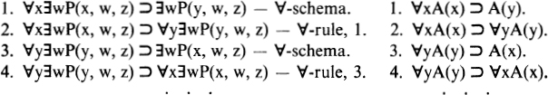
Axiom Schema 9a with 2 and 4 and the ⊂-rule.

For the right column, we shall suppose that x is any variable, A(x) is any formula, y is any variable (not necessarily distinct from x) such that

(i)   y is free for x in A(x),

(ii)   y does not occur free in A(x) (unless y is x),and A(y) is the result of substituting y for the free occurrences of x in A(x). (Recall that (i) means that none of the occurrences of y resulting from this substitution is bound.)

Let us check the requirements that 1-7 be a proof in the right column. They are easily verified when y is x. Now take the case y is not x. For 1, y is the r, and A(y) is the A(r), for the application of the ∀-schema; and using (i) the requirements of the ∀-schema are met. For 2, is the C, and y is the x, of the ∀-rule; and by (ii) the x does not occur free in the C; so again the requirements are met. For 3, we need to see that is of the form , where B(r) comes by substituting r for the free occurrences of y in a formula B(y) and r is free for y in B(y) (then y and B(y) will be the x and A(x) of the ∀-schema). We got A(y) by substituting y for the free occurrences of x in A(x); and by (i) each of the occurrences of y in A(y) resulting from this substitution is free, while by (ii) there are no free occurrences of y in A(x); thus A(y) has free y's exactly where A(x) had free x's, and hence A(x) does come by substituting x (as the r) for the free occurrences of y in A(y) (as the B(y)). Furthermore none of the occurrences of x which enter A(x) by this substitution are bound, as they are simply the original free occurrences of x in A(x). So 3 is justified. For 4, we need merely verify that ∀yA(y) contains no free occurrences of x. This is so because A(y) comes by substituting y for all the free occurrences of x in A(x).

In this example, the left column illustrates the right for the case the A(x) is ∃wP(x, w, z).

EXAMPLE 12.   Now suppose instead that the A(x) of the right column is ∃yP(x, y, z) (with its x and y as the x and y). Then (i) would fail, and the ∀-schema would not be applicable at Line 1. At Line 1 would be . In fact, this formula is unprovable. For, by its truth table for D = {1, 2}, it is not valid, and hence by the theory below (Theorem 12 extended to the predicate calculus in §23), it is unprovable.

Similar examples were given in § 18, where the question whether the conditions of Theorem 15 are met is now synonymous with whether the ∀-schema or the ∃-schema applies.

EXAMPLE 13.   Suppose instead that the A(x) is ∃wP(x, w, y). Then (ii) would fail. Line 1 is correct (i.e. the ∀-schema applies). But at Line 2, the application of the ∀-rule with result would be incorrect, since the x and C of the application would be y and , with the C containing the x free. Indeed, is unprovable.

THEOREM 10 and COROLLARY in §9 again hold, with no change in wording or proof.

EXERCISES.   21.1. Check the left column of Example 11.

21.2. Is the list of formulas a deduction from its first formula? If not, find and explain the mistake.

(a)

         1.   — assumption formula.

         2.   — ∃-schema.

         3.  —∃rule, 2.

         4.   — ⊂-rule, 1, 3.

(b)

         1.   — assumption formula.

         2.   — ∃-schema.

         3.   —∃-rule, 2.

         4.   — ⊂-rule, 1, 3.

(c)

         1.  . — assumption formula.

         2.   — ∃-schema.

         3.   —∃-rule, 2.

         4.   — ⊂-rule, 1, 3.

21.3.   State conditions on x, A(x), y, A(y), C under which the result of Example 9 generalizes to .

21.4.   Add to the following proof to obtain a deduction of from (check all requirements).

State the result which this construction establishes, using the symbol "⊂E". Does the result hold good when P(x), Q(x) are changed to any formulas A(x), B(x)?

21.5. Show that, under the conditions of Theorem 15:

(a) .

(b) .

§ 22. Proof theory: the deduction theorem. We now reprove the deduction theorem (Theorem 11 § 10) for the predicate calculus. Essential use is made of the condition, now incorporated into the meaning of the hypothesis “”, that in the given deduction (α)

of B from A₁,. . ., A_m-1, A_m all variables are held constant.

We use the former proof (§ 10) with some modifications and additions. (The treatment is illustrated by Example 14 below.)

If the last assumption formula A_m is not used (as such) in the given deduction (α), we shall now construct the resulting deduction simply by adding the following at the end of the given deduction: l+1′. – Axiom Schema 1a.

l+2′. — modus ponens (⊂-rule), l′, l+1′.

Now suppose the last assumption formula A_m is used (as such) in the given deduction (α); say the first use of it is B_n, i.e. this is the first of the formulas B₁..., B_l which is justified in (α) on the ground of its being the last assumption formula A_m. We now begin by prefixing "A_m ⊂" only to the formulas B₁,. . ., B_l in the given deduction, to obtain

Now insertions will be required preceding A_m ⊂ B_i, only for i= n... , l, instead of for i = 1,.. ., l. We again specify the method of making these insertions by cases, depending on the reason given for the inclusion of B_i, in (α).

In CASES 1-3 the former treatment applies unchanged. In Case 4, that B_i with i > n comes from B_g and B_h(g, h < i) by modus ponens, we formerly had to provide steps to lead from A_m ⊂ B_g and A_m ⊂ B_h to A_m ⊂ B_i, where B_g, B_h, B_i are of the respective forms A, A ⊂ B, B. (In § 10, these steps were left to the student in Exercise 10.1, but here they are illustrated in Example 14 by 12′-14′ and by 17′-19′.) Now, if g < n we must first supply the following two steps to get A_m ⊂ B_g: — Axiom Schema 1a. A_m ⊂B_g- modus ponens, g′ —. Similarly, if h < n. (This is illustrated by 15′, 16′ in Example 14.) After these preliminaries, the former treatment of Case 4 applies.⁷⁶

CASE 5: B_i with i > n comes from a preceding formula B_g (g < i) by the ∀-rule. So B_g, B_i are of the respective forms C ⊂ A(x), , where C does not contain x free. If g < n, we first supply two steps to get A_m ⊂ B_g, as in Case 4. Remember that i > n, i.e. the application of the ∀-rule comes after the first use B_n of the assumption formula A_m (as such). Hence x does not occur free in A_m; this is by the hypothesis that all variables are held constant in (α), with the definition in § 21 of a deduction in which all variables are held constant. By the stipulation for the ∀-rule, C does not contain x free. Hence A_m & C does not contain x free. This fact is used in justifying the new application of the ∀-rule at k₂+1′ below (top p. 114).

CASE 6: B_i with i > n comes from a preceding formula B_g(g < i) by the ∃-rule. Left to the student (Exercise 22.1).

We have now seen how to construct a particular deduction of A_m D B from A_l9..., A_m___v In this "resulting deduction", all the applications of the V-rule and the 3-rule are on the same respective variables, and occur in the same order relative to the uses of A_l9. .., A_m__x, as the applications in the given deduction. Hence, since all variables are held constant in the given deduction, all are held constant in the resulting deduction. Therefore , as was to be proved.

EXAMPLE 14. As the left column illustrates, , . So by the theorem, . The right column shows the deduction of from resulting by our uniform method from the deduction of ∀xQ(x) from ∀ , ∀xP(x) given in the left column. Because the second assumption formula enters only at 4, the prefixing of “” begins there.

COROLLARY THEOREM 11 follows from the theorem as before.

We now observe that THEOREM 9 (i) and (ii) hold for the predicate calculus with no change in statement.

However (ii) requires a new method of proof. If we simply combined the given deductions as in § 9, it could happen that applications of the ∀-rule or the ∃-rule to variables which occur free in A_l. . ., A_m would come under the first use of A_l. .., A_m in the resulting deduction. By an obvious rearrangement we could mend this with respect to such applications coming from the p given deductions of B₁,. . ., B_p respectively from A_l. . ., A_m. A more serious difficulty is that such applications, with respect to variables occurring free in A_l. . ., A_m but not in B_l..., B_p might come from below the first use of the assumption formulas B₁ . . . , B_p (as such) in the given deduction of C. This difficulty we shall overcome by use of the deduction theorem.

As the hypotheses of (ii) we have: (1) and (2) . Applying Corollary Theorem ll_Pd to (2):⁷⁷ (3) . Now we build a deduction of C from A_l . . ., A_m as follows. Take the p deductions of B₁ . . ., B_p respectively from A₁,. . ., A_m (which exist by (1)); write them consecutively; and then move to the front of the combination the part of each which precedes the first use in it of an assumption formula (as such). To the sequence of formulas thus obtained, prefix the proof of (which exists by (3))). Finally, suffix applications of modus ponens which lead from .

In the deduction of C from A_l . . . , A_m thus constructed, there are no applications of the ∀-rule or the ∃-rule coming below uses of the assumption formulas (as such) except ones which came in from such applications in the deductions given by (1). By the hypothesis (implicit in our using“⊃E” without superscripts) that all variables are held constant in those deductions, the variables for these applications do not occur free in A₁ . . ., A_m. Thus in our deduction all variables are held constant, so .—

Having reinstated Theorem 9, we now have all the general properties of (written without superscripts) that were noted in § 13.

EXERCISES. 22.1. Treat Case 6 in the proof of the deduction theorem.

22.2. Is the deduction theorem applicable to 3-12 of Example 14 as the“given deduction” (with 3 justified by "assumption formula")?

§23. Proof theory: consistency, introduction and elimination rules. The.corollaries to Theorems 10_Pd and 1_Pd in §§ 21, 22 reduce the notion of deducibility "" to that of provability " E" in a manner parallel to the reduction by Corollary Theorem 8_Pd in § 20 of valid consequence "" to validity " E".⁷⁷ (Likewise, using ∀′, we have parallel reductions of "" and "".) So now to show the equivalence of model theory and proof theory for the predicate calculus, it remains to show that E if and only if E.

The “if” part is easy. THEOREM 12 and COROLLARY of § 11 hold again. The proofs are as before, using now 1a-10b in Theorem 2 _Pd, and Theorems

3_Pd, 15 and 16, in § 18. The present corollary does not require the full force of the theorem, which refers to any D. It can be inferred from the theorem with “” replaced by "", i.e. using only D = {1}. This is the way the simple consistency of the predicate calculus was first proved by Hilbert and Ackermann in 1928.

The “only if” part, E only if E (extending Theorem 14 to the predicate calculus), is not as elementary as the theorems we have thus far given. This proposition is included in Gödel’s completeness theorem 1930, which we shall postpone to Chapter VI (Theorem 37 § 51).

In classical logic (with which we are primarily concerned), we are interested in the valid formulas because they express universal logical truths, and in the provable ones because they are valid.

In the case of the (classical) propositional calculus, constructions of truth tables (or truth-value analyses, § 8) constitute a sure and unimpeachable method of demonstrating validity, directly from its definition in model theory. However, this method isn't always very practical, and it usually doesn't resemble actual thought processes, in which the utmost economy is essential. This is partly why we introduced also proof theory. Of course, we didn’t stop with the postulated form of proof theory, but we proceeded thence to derived rules (§ 13). The postulated form of proof theory can be regarded there as a very convenient way station between model theory (validity, etc.) and the derived rules of proof theory.⁷⁸

Now, in the (classical) predicate calculus, direct application of the definition of validity is no longer a simple matter. For, demonstrations of validity by considering the truth tables are no longer purely mechanical, but require general reasoning about the truth tables for all (non-empty) domains D; and for infinite Z>’s, the truth tables are infinite objects.

Hence, in the predicate calculus, proof theory has the advantage over model theory, not only of convenience, but of greater concreteness. We are on firmer ground in establishing provability from its definition in § 21, with the help of elementary theorems such as the deduction theorem and results based on the proof theory of the propositional calculus, than in demonstrating validity from its definition in § 17. By Theorem 12_Pd, demonstrations of provability do establish validity, for anyone who accepts the reasoning in its proof.⁷⁹

Gödel’s completeness theorem for the predicate calculus has the significance that, for all true statements of validity, this method of demonstration suffices. In using this method, we escape from having to reason further in terms of the validity notion, after handling the few cases of it that we needed for the proof of Theorem 12_Pd. Demonstrations of all other true statements of validity can be put together out of repetitions of the reasoning used in handling those few cases.

Because of our preference for the proof-theoretic approach to the predicate calculus on the ground of its greater concreteness, we now develop some of the further results proof-theoretically, including some which in Chapter Ior § 19 we did model-theoretically.

THEOREM 13 again holds. For, as we remarked early in § 21, the direct rules carry over automatically from the propositional to the predicate calculus; and the three subsidiary deduction rules in Theorem 13 are established now by the same proofs from Theorem ll_Pd in § 22 as before from Theorem 11. We now add four more derived rules.

THEOREM 21. Let x be any variable, A(x) be any formula, r be any variable not necessarily distinct from x,and A(r) be the result of substituting r for the free occurrences of x in A(x). Also let Γ be any list of (zero or more) formulas, and C be any formula. Then the following rules hold, provided:

(A)   For ∀-elimination and ∃-introduction, r is free for x in A(x).

(B)   For ∀-introduction and ∃-limination, Γ does not contain x free.

(C)   For ∃-elimination, C does not contain x free.

There is some arbitrariness whether our particular set of postulates or some other is accepted. The problem of completeness (solved by Godel, e.g. for our postulates) only appears to a person who is not merely accepting a set of postulates as the starting point of logic.

PROOFS. ∀-elimination, ∃-introduction. Cf. Exercise 21.5. ∀-introduction. Let C be an axiom not containing x free.

1.   — by hypothesis.

2.   — Exercise 13.2, 1.

3.   — Theorem 1 _Pd, 2.

4.   — from 3 using the ∀-rule, or in more detail thus: Consider a given deduction B₁ . . ., B_l of C ⊂ A(x) from Γ with all variables held constant. To this we can add as B_l+1 the formula , justified by the V-rule with B_l as premise, since C does not contain x free. In the resulting deduction from Γ, all variables are held constant, since the new application of the ∀-rule is on x, which by Proviso (B) does not occur free in Γ

5.   — Theorem 10_Pd (or modus ponens), 4.

6.   — Exercise 13.2, 5. ∃-elimination.

1.   — by hypothesis.

2.   — Theorem ll_Pd, 1.

3.   — from 2, using the ∃-rule (and Provisos (B), (C)).

4.   — Theorem 10_Pd, 3.

In Exercise 23.1 below we shall illustrate the importance of watching Provisos (B) and (C) in using these rules. The importance of (A) should appear from examples in §§ 21 and 18 which deal with essentially the same matter.

The subsidiary deduction rule of ∀-introduction is unlike our other subsidiary deduction rules in having the same assumption formulas in the given or subsidiary deduction and the resulting deduction. It is stated as a subsidiary deduction rule because of Proviso (B). Except for this proviso, Example 13.3 would apply and give "". That however does not hold; for then, by Theorem 12_Pd (with Theorems ll_Pd and 8_Pd) we would have ""; and this is not the case e.g. when A(x) is P(x) or (as we saw in Example 7 § 20) —≠P(x).

COROLLARY 1.   Let w₁. . ., be distinct variables, A(w_l..., ) be a formula, r_l. . ., be variables not necessarily distinct from each other or from w₁. . ., , and A(r_l . . . , ) be the result of substituting r_l. . ., simultaneously for the free occurrences of w_l. . . , respectively in A(w₁,. . ., ). If this substitution is free (i.e. if the resulting occurrences of r₁ ..., in A(r₁. .., ) are free), then:

(a)   . (p-fold ∀-elimination.)

(b)   . (p-fold ∃-introduction.)

PROOFS, for p > 1. (For p = 0, (a) and (b) are simply Theorem 9_Pd (i) for m = 1. For p= 1, they are in the theorem.) (a) For illustration,

suppose p = 2, and w₁, w₂ are x, y, and A(w₁, w₂) is ∃wP(w, x, y), and r_l, r₂ are y, z. Then the substitution is free. (It would not be if r_l, r₂ were w, z.) We must show that . Evidently we should use ∀-eliminations, but a little care is necessary. We cannot first eliminate ∀x with y as the r to obtain , as the resulting occurrence of y (the second) would not be free. To use an easily-described uniform method, let x_1? x₂ be two distinct new variables, i.e. variables distinct from each other and all the others in the illustration. By two successive V-elims. (with Theorem 9_Pd (ii)):

(1)  . Thence by two successive ∀-introds.: (2) . By two successive ∀-elims.: (3) . Combining (2) and (3) by Theorem 9_Pd (ii): (4) (b) Left to the student (Exercise 23.2 (b)).

COROLLARY 2.   (Substitution for individual variables.)⁶³ Under the circumstances of the theorem or Corollary 1, and provided Γ does not contain free occurrences of x or w₁,. . . , respectively:

(c)   If then .

(d)   if then .

PROOF is Exercise 23.3.

EXERCISES.   23.1. In each of the following, the formula in the last statement is not valid (by Exercises 17.3, 17.5) and therefore (by Theorem 12_Pd) not provable, contrary to what is asserted. Locate the fallacy.

23.2.   (a) Write out the six ∀-elims. and ∀-introds. in the illustration of the proof of Corollary 1 (a), and verify that the provisos are satisfied. (b) Give the proof of Corollary 1 (b) with the same illustration.

23.3.   Prove Corollary 2. Also simplify the statement for the case Γ is empty.

23.4.   Show that: For each variable x and formula A, A if and only if ∀xA; and hence, A if and only if ∀A (cf. § 20 for "∀").

23.5.   Show that: if and only if (where as in § 20).

23.6.   True or false (and why)?

(a)   "."

(b)   "."

23.7.   For each of the following modifications of the predicate calculus, say which of the two implications (Theorem 12_Pd and
Chapter VI) continue to hold for all formulas E, and why.

(a)   Add as a new axiom schema .

(b)   Add as a new axiom schema .

(c)   Omit the ∀-schema, ∀-rule, ∃-schema and ∃-rule.

§ 24. Proof theory: replacement, chains of equivalences .

Theorem 22. Let x be any variable, and A, B, C, A(x), B(x) be any formulas, and for *69a-*72a let "image" be any list of {zero or more) formulas not containing xfree.⁸⁰

(Intrduction of a logical symbol into an implication, including contraposition with double negations supressed.)

(Intrduction of a logical symbol into an equivalentce)

(Special cases of the binary propositional connectives.)

PROOFS. All of the results except the four involving quantifiers (*69a-*72a) can be established in the propositional calculus. This can be done automatically with , by truth table computation with P, Q, R, followed by substitution in the form of Exercise 7.3 ;⁸¹ and then can be changed to h by completeness (Theorem 14 with Theorems 8, 10); or we can use the rules of Theorem 13, employing *6-*12 in the proofs of *26-*30. Then they can be taken over into the predicate calculus, by beginning § 21. (Exercise 24.1.)

*69a, *70a. *70a is the result of Exercise 21.4, when we employ a deduction of A(x) ⊂ B(x) from Γ instead of from . *69a is obtainable similarly, or by generalizing Example 14 from P(x), Q(x) to A(x), B(x) and replacing the first three steps by the assumed deduction of A(x) ⊂ B(x). Or we can use the rules of Theorems 13 and 21 (Exercise 24.2).

*71a, *72a. *71a is established as follows, and *72a similarly.

1.   — hypothesis; ∼-elim.³⁵

2.   — *69a, 1.

3.   — similarly.

4.   — ∼-introd., 2, 3.

Now we can extend Theorem 5 to the predicate calculus with "Γ in place of " (The extension with "" is in § 19.)

THEOREM 23. (Replacement theorem.) Let C_A be a formula containing a formula A as a specified (consecutive) part, and let C_B come from C_A by replacing that part by a formula B. Let x_l . . ., x_q be the free variables of A or B which belong to quantifiers of C_A having the specified part within their scopes (i.e. x_l. . . , x_q are the variables having free occurrences in A or B which become bound occurrences in C_A or C_B). Let Γ be a list of (zero or more) formulas not containing any of x_l...x_q free. Then:

.

PROOF. We illustrate the proof by four examples.

EXAMPLE 15.   Let C_A be with the specified part A underlined. Let“” be “” (with Γ empty), which holds by *82a in Theorem 26; i.e. the formula 1 below is provable. Using *29a, *71a and *27 we infer successively that 2-4 are also provable.

Thus , which is what the theorem asserts in this example.

EXAMPLE 16. Let C_A be with the specified part A underlined. Let"" be "", which holds by double ∀-elim.; i.e. the formula 1 below is deducible from the Γ Using *26, *72a (since the Γ does not contain y free), *71a (since x isn't free in Γ), *29b, we infer successively that 2-5 are also deducible from the Γ.

Thus , which is what the theorem asserts in this example.

EXAMPLE 17.    In Example 16 change B to . Since w does not become bound in replacing the specified P(x) by , it is permitted to be free in the Γ Thus .

EXAMPLE 18.   Changing the specified occurrence of P(x) in Example 16 to be the first one, C_A ∼ C_B is deducible from P(x) ∼ B (using simply *29a), whatever the B.

COROLLARY 1. For C_A, C_B, x_l..., x_q as in the theorem:

PROOF.   Apply the theorem with as the Γ, as in Examples 16, 17. Remember that “” means “”.

COROLLARY 2.   (Replacement property of equivalence.) Similarly:

(a)   If , then Γ C_A C_B.

(b)   .

Now we can return to (α)-(Ζ) in § 5, and verify that they hold with "" replaced by "Γ " (Exercise 24.3). So with Theorem 23 (or its Corollary 1), we have all the ingredients for using chains of equivalences in proof theory, with "Γ " standing before the chains (instead of "" as in §§ 5, 19). The formulas Γ must not contain free any of the variables x_l. .., x_q of quantifiers within the scopes of which replacements are performed (or such variables which they do contain free must be written as superscripts on ""). In most of our applications (e.g. those in the proofs of Theorems 25 and 26), Γ is empty (as in Example 15); i.e. the equivalences are provable, and we need not worry about x₁,.. ., x_q.

Suppose that in C_A (as in Theorem 23) the specified part A is not in the scope of any ∼ (i.e. it is not in the D of any part D ∼ E or E ∼ D). We then say the specified part A is positive or negative according as it is in the D of an even or odd number of parts of the form ≠D or the form D ⊂ E. For example, in the part P(x) is odd (count the underlined operators), and the part Q is even (count the overlined operators).

THEOREM 24.   Under the circumstances of Theorem 23, and supposing further that the specific part A is not in the scope of any ∼

If , then if the specified part A is .

COROLLARY. if that part A is.

PROOFS is Exercise 24.4.

LEMMA 5.   Let x be any variable, A(x) be any formula, y be any variable (not necessarily distinct from x) such that

(i)   y is free for x in A(x),

(ii)   y does not occur free in A(x)(unless y is x),andA(y) be the result of substituting y for the free occurrences ofx in A(x). Then:

*73. .   *74. .

PROOFS.   *73. By the right column in Example 11. *74. Similarly.

THEOREM 25. If A is congruent to B, then .

PROOF.   We illustrate this by the example (1) and (2) of congruent formulas end § 16. In order to employ a uniform method applicable in all cases (though short cuts will generally be available in particular cases), we pick a set of new variables x_l9 x₂, x₃ to correspond to the three quantifiers of either. By successive replacements of the variable-occurrence bound by one quantifier at a time, we can transform 1 (= (1)) into 4 (cf. (lb), (2b)) and that into 7 (= (2)), thus:

The proof that (here A is (1) and B is (2)) is given by the chain method. E.g. for the "third link", the hypotheses of Lemma 5 are satisfied by x, , x₃ as the x, A(x), y; so by *73 the underlined parts of 3 and 4 are equivalent (i.e. the formula expressing their equivalence is provable); so by Theorem 23, 3 is equivalent to 4.

EXERCISES.   24.1. Run through all steps in the proofs of *6, *7 and *26 by each of the suggested methods.

24.2.   Establish *69a and *70a by the rules of Theorems 13 and 21.

24.3.   Verify that (α)-(Ζ) in § 5 hold for the predicate calculus with "Γ ". (For (β)-(Ζ), cf. *19-*21 in Theorem 2.)

24.4.   Prove Theorem 24 and Corollary.

24.5.   Justify the following. Format (B₁) § 13 Is used in (b).

(a)   1. .

         2.  .

         3.  .

This expresses the traditional Aristotelian syllogism "Baroco": All P are M. Some S are not M. Therefore some S are not P.

(b)   Assume . Thence successively , . — Thus

("Festino").⁸²

§25. Proof theory: alterations of quantifiers, prenex form.

We shall use the proofs for Theorem 26 below to provide further illustrative and practice material in the technique of § 13 for using our derived rules. Formats "(A)", "(B₁)", "(B₂)", "(B₃)" are used as there. Now we have in addition the four introduction and elimination rules for the quantifiers (Theorem 21). The provisos for these rules must be observed carefully, as always.

The rule of ∀-introduction was stated in Theorem 21 as a subsidiary deduction rule in which the assumption formulas are not changed from subsidiary to resulting deduction. The effect is that, when we are listing formulas deducible from assumptions Γ not containing x free, we can proceed by ∀-introduction from A(x) to ∀xA(x).

The rule of ∃-elimination serves to eliminate the ∃x from ∃xA(x) preparatory to inferring from ∃xA(x) (and possibly other assumptions Γ not containing x free) a consequence C not containing x free. The procedure corresponds to the following familiar form of reasoning in mathematics:“There is an x such that A(x); now pick such an x;. . .” or "There is a number with the property A; let x be such a number . . .". If through a chain of reasoning using x a conclusion is reached not containing x, the conclusion can be taken to be established without the assumption about x.

One of the purposes of studying logic formally is to improve our reliability in the use of logic. This improvement is obtained by our being able, in cases of doubt, to trace how our proposed reasoning (or the reasoning of others) can be effected by the principles we have studied, or in brief how the reasoning can be "formalized". Also, as will appear in Chapter IV, we may sometimes wish to do so to make clear the bases of the reasoning, whether or not we have doubts about its validity.

Therefore, it is an objective of the formal study of logic to bring the methods of recognizing that formulas are provable in the strict sense of proof theory (§§ 9, 21) as close as possible to the methods which are used informally.

This we imdo not claim can be done once and for all, for all kinds of reasoning. However, in our opinion, the rules for introducing and eliminating logical symbols do this very successfully for the ordinary use of predicate logic, not just for proving results within logic (as in our next illustrations) but also in the application of logic in mathematics and elsewhere. The remarks at the end of § 13 on supplementing these rules appropriately by other devices should be kept in mind.

The introduction and elimination rules are due essentially to Gentzen 1932, 1934-5, 1936 § 5 (who profited from earlier work of Hertz 1929) and Jaskowski 1934.⁸³ These authors were primarily interested in formulations of logic with such rules as postulated rules, while we have them as derived rules; cf. § 13. Our format (B₂) corresponds closely to Gentzen’s“natural deduction” and Jas´kowski 1934.

It is controversial whether one does better to start with a postulated formulation of logic based on modus ponens (a "Hilbert-type system",§§ 50, 54) and derive the introduction and elimination rules, as we have done, or to start out with a version of the latter as the postulated rules (a "Gentzen-type system").

No one formulation is most convenient for all purposes. One formulation with postulated axioms and rules is necessary to give a firm starting point for proof theory. But it is our view that, no matter what formulation one begins with, he will not want simply to use it, but rather he will soon wish to escape its limitations by devising short cuts, proving theorems that introduce new methods, etc. The history of mathematics is one of continually building on previous discoveries, and of devising methods which telescope or reorganize steps previously carried out separately into new processes of reasoning.

This being the case, we have preferred to start from the structurally simpler Hilbert-type systems in §§ 9, 21. These also lend themselves well to the addition of mathematical axioms and axiom schemata to establish systems of logic and mathematics, of which we shall have more to say in Chapter IV.⁸⁴

THEOREM 26. Let x, y be any (distinct) variables, A(x), B(x), A(x, y) be any formulas, and A, B be any formulas not containing x free. For *79 and *80, further let A(x, x) be the result of substituting x for the free occurrences ofy in A(x, y), and suppose that y is free for x in A(x, y) (i.e. the occurrences of x in A(x, x) resulting from this substitution are all free).⁸⁵

PROOFS.

         *75. 1. ∀xA A — ∀-elim. (with x as both the x and the r and A as the A(x), so trivially the r is free for the x in the A(x)).

— ⊂-introd., 1.

4.   — ∀-introd., 3 (which is legitimate since A does not contain x free).

5.   — ⊂-introd., 4.

6.  — ∼-introd., 2, 5.

I. Assume ₁∀xA (preparatory to ⊂-introd.). By ∀-elim., ₂A.

(B₁)   II. Assume ₄A, which does not contain x free. So by ∀-introd., ₅∀xA.

*76. 1. A A.

  2. ∃xA A — ∃-elim., 1 (noting that A as the C does not contain x free).

(A) 3. — ⊂-introd., 2.

  4.   — ∃-introd. (with x as the r).

  5.   — ⊂-introd., 4.

  6.   — ∼-introd., 3, 5.

*80. 1. — ∃-introd. twice (first with y as the x and x as the r, using the hypothesis that x is free for y in A(x, y); then with x as both the x and the r); or by Corollary 1 (b)

(A) Theorem 21.

2.   —∃-elim., 1 (noting that as the C does not contain x free).

3.   — ⊂-introd., 2.

*82a. 1. .

2.   — ∃-introd. (with x as the r).

3.   — ≠introd., 2, 1.

4.   — ∃-introd., 3 (noting that as the T does not contain x free).

5.   — – ⊂-introd., 4.

6..

(A) 7.   — ∀-elim.

8.   — weak ≠-elim., 6, 7.

9.   — ∃-elim., 8 (noting that neither as the C nor as the Γ contains x free).

10.  .

11.   — ≠-introd., 10, 9.

12.  — ⊂-introd., 11.

13.   — ∼-introd., 5, 12.

I. Assume ₁. Preparatory to reductio ad absurdum (≠-introd.), assume ₂A(x). By ∃-introd., ₃∃xA(x), contradicting ≠∃xA(x). So by the ≠-introd. (discharging the assumption A(x)), ₄≠A(x). By ∀-introd. (as the remaining assumption doesn’t contain x free), ₅. II. Assume ₇. For ≠-introd.,

(B₁)   assume ₈∃xA(x). Preparatory to ∃-elim., assume ₉A(x). From by ∀-elim., ₁₀≠A(x), contradicting A(x). By weak ≠-elim., ₁₁. Since neither this formula nor the assumption formulas , ∃xA(x) other than A(x) contain x free, we can now complete the ∃-elim., and then (noting the contradiction to ) the ≠-introd., to obtain ₁₃≠∃xA(x).

At each step the results in (B₂) which are opposite no other arrows are available. Thus for 4, we can use 1 as one of the two“given deductions” for the ≠-introd., since from we have (by general properties of ) A(x), . Though we could suspend the assumption ∃xA(x) for Lines 9-11, we prefer to keep it in force throughout Lines 8-12, so the immediate result of the ∃-elim. applied to 11 is ∃xA(x), ∃xA(x), . (Cf. Lines 12-17 in (B₃) of Example 9 §13.)

*82b.   We use the chain method (available by § 24). .

*87-*94.   All of these can be established in pairs, as we illustrate next for *91 and *92. (Also *88, *90, *94 can be established by direct methods, like *91.)

*91. I. Assume for ⊂-introd., ₁A &∃xB(x). Thence by &-elims., ₂A and ₃∃xB(x). Assume for ∃-elim., ₄B(x). By &-introd., ₅A & B(x). By ∃-introd., ₆∃x(A & B(x)). Now complete the ∃-elim. and ⊂-introd.

(B₁)   II. Assume ₉∃x(A & B(x)). Assume for ∃-elim., ₁₀A & B(x). By &-elims., ₁₁A and ₁₂B(X). By ∃-introd., ₁₃∃xB(x). By &-introd., ₁₄A & ∃xB(x). Complete the ∃-elim. and ∼-introd.

*92. [*56] ∼

*95-*99b.   These can all be obtained by the chain method from *88 *90, *92, *94 via *59 , *82a, *82b (and *34). The transformations can be performed mentally (with a little practice), so this can be used to remember them from *88-*94. (Also some of them can be established by direct methods.)

It can be remembered that *87 and *88 hold rather than the similar formulas with ∀ and ∨ or with ∃ and & (cf. *94, *93), since ∀ and & are kindred operations (∀ can be thought of as a conjunction extended over D; e.g. if D = {1, 2, 3}, then ∀xP(x) is synonymous with P(l) & P(2) & P(3) in the extension of the predicate calculus having the symbols "1", "2", "3" as names for the members of D), and so are ∃ and ∨.

THEOREM 6° and COROLLARY° now extend to the predicate calculus with (instead of ), where the operation † now includes the interchange of ∀ with ∃. The proof is as before, now using also *82a and *82b.⁸⁶

A prenex formula is one with all its quantifiers (if any) at the front, with all the rest of the formula as scope of the prefixed quantifiers. Thus is prenex but not . If E is equivalent to F (i.e. E ∼ F) and F is prenex, F is a prenex form of E.

THEOREM 27°  . Each formula E has a prenex form.

PROOF. Say for example E is . We can transform this E to a prenex formula F by a chain of equivalences, thus:

In the first application of *92 (with *34), ∀xQ(x) (which does not contain x free) is the A and ≠P(x) is the B(x). Then we use Theorem 25 to replace ∀xQ(x) by ∀yQ(y), so that in the final application of *92 (with y as the x) the A will not contain the x free.

THE INTUITIONISTIC PREDICATE CALCULUS. (Cf. end § 12.) Simply by using Axiom Schema 8¹ in place of Axiom Schema 8 (i.e. basing the predicate calculus on the intuitionistic propositional calculus instead of on the classical propositional calculus), we obtain the intuitionistic predicate calculus (proof-theoretically). Results established using only the derived rules of Theorems 13 and 21, except double negation elimination, hold good for it.⁸⁷

Exercises. 25.1. Translate the following from the format (B₁) and (B₂), and check that all steps in (B₄) are correct.

(a)    The proof of *91 given above.

(b)    The following proof of *96: I. Assume (preparatory to introd.) B. Assume (for introd.) A(x). By introd. , and by elim. B. By introd. (discharging the assumption A(x)), A(x) B. By introd., B). II. Assume B) and . By elim. from the former, A(x) B. Assume preparatory to elim. from the latter, A(x). By elim., B.

25.2. Give proofs of *82 and *90 by direct methods in the format (B_x), and rewrite them in the formats (B₂) and (B₃).

25.3. Attempt similar treatment, and locate the fallacy. (Reduce the step in question to a proposed explicit application of one of the introduction and elimination rules, and show what requirement would be violated.)

(a)   The converse of *82 (Vy3xA(x, y) D 3xVyA(x, y)). (Cf. Example 3.)

(b)   *92.⁸⁸

25.4. Prove *83, *95, *98 from earlier results by the chain method.

25.5. Prove *99b from *94, and also give a direct proof in the format (B1).

25.6. Give proofs in the format (B₁) of:

(a) (cf. *82b).

(b) & & B(x)).

25.7°. Establish h V B(x)) D .

25.8*. Show that *80 does not hold in general without the restriction stated in the second sentence of the theorem.

25.9. Show that *91 does not hold in general without the restriction
that A not contain x free.

>25.10. Do Exercise 19.4 with“A is equivalent to B” now meaning .

25.11. Reduce to prenex form:

(a)    &.

(b)   . Save steps by applying Theorem 6_Pd to the result of (a).

(c) . Come out with only two quantifiers.

(d)   . Use *63a first.

25.12°*. (a) Prove the theorem:⁶⁶ For each formula E andO-place ion P: h E ~ (P & F₁) V (~iP & F₂) where F_iis P or P or a formula not containing P (i= 1, 2).HINT: Use *49, *40a-*48 (in § 24), *75, *76, to obtain F_l F₂ as described such that P E F₁ and P E ,F₂.

(b)   The theorem comprises 9 (= 3 ? 3) cases, since each of F_x and F₂ can have one of three forms. Simplify (P & F₁) V (P & F₂) in 8 of these cases.

(c)   State and establish a similar theorem with two 0-place ions P₁ and P₂ in place of one P.

*§ 26. Applications to ordinary language: sets, Aristotelian categorical forms. We continue from §§ 14, 15. Now a richer system is available for our logical analyses: the predicate calculus, or more specifically the restricted, one-sorted, classical predicate calculus, §§ 16, 17.

In translating verbal expressions into logical symbolism, we must as before (§ 14) set clearly before ourselves the interpretation, or possible models, of the symbolism.

So, when a translation using only the propositional calculus will not suffice, we must be able to regard all the sentences for the given application of the predicate calculus as speaking about the members of some one nonempty set D. After translating, we will test the translated argument for validity without assuming that we know what nonempty set D is. Therefore, we are not compelled before translating to be specific about what D is, so long as we agree that there is some nonempty set D to which all the objects under discussion belong, and which can serve as the range of the variables in the translations of statements using "all", "some", etc.

Having envisaged a D, we must next be able to select a list of predicates, i.e. of propositional functions (each of some number n > 0 of variables), as the independent basic predicates which the sentences concern; no one of these predicates is to be regarded (for the purpose of our analysis) as composed out of other predicates. Each of these predicates, when each of its variables becomes (or takes as value) a member of D, is to become (or take as value) a proposition, which is either true or false (but not both). We then establish the symbolism for our application of the predicate calculus by picking prime predicate expressions or ions, which we usually write from the beginning with attached name form variables, to express these predicates.

In these two steps, of picking a D and of picking predicates over D which take values that are each either true or false, we may be representing what we believe to be the actual situation, or we may be making simplifying assumptions to enable us to reason exactly.

Let us digress for a moment to introduce a little standard terminology about sets. We do not undertake now to criticize the notion of a“set” or“collection” or“aggregate” or“totality” or“class” C, as constituted by objects thought of together and said to“belong” to C or to be“members” of C or“elements” of C. We assume the reader has a sufficient understanding of this for present purposes. We write“ ” to say that x is a member of C; and“ ” to say that x is not a member of C (i.e.“” abbreviates ).

A set is to be completely determined by what objects are members of it. Thus C₁ and C₂ are the same set exactly if the same objects belong to each; in symbols C₁=C₂ if and only if .

A set C is included in a set D or C is a parf of Dor C is a subset of D, or in symbols C D, exactly if each member of C is a member of D. In symbols, CDif and only if . (Then C = D if and only if For any set D, this definition makes D itself a subset of D; we call D the improper subset of Z). Any other subset C of Z), i.e. any set C such that every member of C is a member of Z), but some member of D is not a member of C), we call a proper subset of Z), and write C D). The set containing no objects as members, which we call the empty set, is a subset of every set D).89

For example, suppose D is the set of three elements a, b, c; in symbols, D = {a,b, c}. Then D has eight subsets:

The first { } is the empty set; the last {a, b, c} the improper subset of D; and the second, third and fourth {a}, {b}, {c} are unit sets, i.e. sets with just one element each.

The domain D for an application of the predicate calculus may also be called the universal set or the universe or universe of discourse. It is to be simply a set, fixed for the given application, which contains as members all the objects which we are considering in that application. Thus, if a given piece of reasoning concerns natural numbers 0, 1, 2,. . . and no other objects, then D can be the set of all the natural numbers, but need not include shoes, ships, sealing wax, cabbages and kings. In the following example, which we didn't successfully analyze in § 14, it wouldn't do to take D to be just the natural numbers.

Example 19.“All men are mortal. Socrates is a man. Therefore Socrates is mortal.” If D, including Socrates, whom clearly we are talking about, were just all men, the second sentence would be unnecessary to the argument. If the set D of all the objects we are talking about, including Socrates, were by definition exactly the mortal objects, the argument itself would be redundant. So we had better think of D as consisting of, say, the "beings", which includes men, mortal objects and maybe more (as in Greek mythology, gods). D could include natural numbers and minerals, if "a; is mortal" is construed as meaningful when x is a natural number or a mineral; but this seems far fetched. Using H(x) to express "z is a man" (human being), M(x) to express "x is mortal", and s to express "Socrates", the argument can be symbolized thus:90

To say that this is correct reasoning would mean that

(cf. § 20). We have chosen (2) rather than

because in (1) as a rendering of the verbal argument the variable s is supposed in both H(s) and M(s) to name the same member of D, i.e. Socrates. The reader will have no trouble in establishing (2) directly, or (by beginning § 23) via

Since thus far we have been doing without“constants” as symbols separate from variables, it was important here to give s in (1) and thence in (2) the conditional interpretation ((I) in § 20). We could avoid any uncertainty about the status of free variables in premises by writing the premises in the form where V is closure with respect to all variables not intended to be held constant. This probably corresponds best to usage in ordinary language (outside of mathematics), where constructions equivalent to the use of free variables not held constant scarcely occur. However, in mathematics premises are very often stated with free variables having the generality interpretation ((II) of § 20), e.g. x+y = y+x and . Hence we see no reason not to allow this practice here. We can avoid ambiguity then by writing the variables x₁,. . ., x_q which are not necessarily held constant as superscripts on “∴”, just as we did on “” beginning in § 20, and on " " in § 21.

The requirement that all the objects considered belong to one nonempty set D called the domain, does not prevent our talking about the members of other sets C_l C₂, C₃,. . ., provided those other sets are included in D (i.e. provided Thus we can regard Example 19 as dealing with three sets D = {the beings}, H={the humans} = {the x's in D such that H(x)} = , M = {the mortals} = {the x's in D such that M(x)} = .⁹⁰ As this illustrates, to each one-place predicate C(x), where the variable x ranges over A we can define a subset C of D as containing just those x's for which C(x) is a true proposition; in symbols, .⁹¹

Inversely, if we have first introduced some subset C of A we can define a predicate C(x) by C(x) = . In particular, if the sets H of humans and Af of mortals (as subsets of D) were first introduced, then“H(x)” and“M(x)” could be considered as standing for and respectively.⁹²

Notice that in (1)-(3) the subsets H and M of D are mentioned via the ions H(—) and M(—). But D itself is not mentioned explicitly; D enters implicitly, as the range of the variable x, and also of s in the validity treatment, where we disregard its interpretation as naming Socrates.

Example 20. "Every odd natural number is a difference of two squares. 5 is an odd natural number. Therefore 5 is a difference of two squares". For this argument, no objects need to be considered which are not natural numbers. So let us take the domain D = {the natural numbers}. Using O(x) for "x is odd", and D(x) for "x is a difference of two squares", and f to express 5, we obtain the symbolization:

Apart from the letters used, this is the same as (1) in Example 19; so the argument is valid. (The demonstration of validity there encompasses both the argument about Socrates and the argument about five.) The D of this application is quite precise (or so mathematicians usually think), while that of Example 19 is a rather vaguely defined totality.

This example is similar to the second illustration [2] for material interpretation early in § 2. We weren’t ready there to talk explicitly about a domain D (say the positive integers > 1) or to use a quantifier Vx. So there we let n be a number which was fixed by being written on a paper in your pocket, but was unknown to me. So my assertion could be considered as simply OF, where O is "n is odd" and F is "xⁿ + yⁿ is factorable" for that fixed n. But since I was in ignorance of the particular number n in your pocket, I had to consider all the possibilities. Using our present notation, I can now say that, before risking a wager with you, I convinced myself of , where D = {all positive integers > 1}, O(x) is "x is odd" and F(x) is "xⁿ + yⁿ is factorable". Thence I passed by elimination to O(x) F(x) (or briefly OF) with x referring now to the number n in your pocket. In this illustration, material implication , used in combination with a universal quantifier, enables us to make the statement about just the odd positive integers > 1, while using a variable x that ranges over the set of all positive integers > 1. We are able to do this because we made the truth table for A B give t whenever A is f. The relationship between propositional functions 0(x) and F(x) (rather than just propositions) expressed by is called “formal implication”. Similarly, expresses“formal equivalence” between propositional functions P(x) and Q(x). —

In the logic of Aristotle (384-322 B.C.) and his followers, down into the nineteenth century, a paramount role was given to four forms of statement called “categorical”. We show these forms below at the right, and our symbolizations of them at the left. Here S(x) stands for “x possesses the property S” and P(x) for “x possesses the property P”. The first premises in Examples 19 and 20 illustrate the A form.⁹³ In these forms, when S is expressed in the singular,“are” becomes“is”. “Every” or“each” can replace “all”.

We have stipulated that the range of our variables, here x, be some nonempty set D. But, in the symbolizations of the first two forms, the effect of "S(x)" is to remove from our attention the part of D outside the set S, so that the assertion that P(x) holds (first form) or fails to hold (second form) is made only for

If for the moment we allow a second sort of variables, where x ranges over D is synonymous with where £ ranges over S (with SD); and is synonymous with . Similarly, in the third form is synonymous with ; and in the fourth 3x[S(x) is synonymous with .

It would not be worth while to complicate the symbolism by introducing a second sort of variables, unless we were to make a great deal of use of them. (For simplicity in this book, we are avoiding them in any case.) So we now revert to the one-sorted predicate calculus, in which we can get the effect of a variable over a subset of the domain D by prefixing S(x) D to the scope of a universal quantifier and S(x) to the scope of an existential quantifier.

We excluded the empty set as a possible choice of D. This only means that the (complete) range of our variables is not to be empty; there is to be at least one value of x. But when we confine our attention to a subset of D by using , this subset S may be empty. I may develop the theory of angels in our form of the predicate calculus; but if I am in doubt whether angels exist, I shall first have to embed the set S of angels in some totality D that I am sure is not empty.

Under our translations, when S is empty,“All S are P” and“All S are not-P” are true, while“Some S are P” and“Some S are not P” are false. For example, on the supposition that there are no angels, we can truthfully assert“All angels have wings” and also“All angels are wingless” or equivalently "No angels have wings".

This is a point on which ordinary language is ambiguous, just as in everyday speaking“or” is sometimes intended inclusively and sometimes exclusively. People wouldn't ordinarily say“All S are P” if they already knew that S is empty; but they might say it when they were in ignorance that S is empty or had not considered that possibility. Then if confronted with the fact or possibility that S is empty, they might disagree on whether to regard“All S are P” as true in that case (as we do) or as false. Indeed, Aristotle took the latter interpretation; i.e. he took“All S are P” to include the assertion that there are some S. Under Aristotle's interpretation, the translation of“All S are P” into our symbolism is .94When S is nonempty, i.e. when is true, this is equivalent to our . (By *45 in § 24,

Our reason for preferring to use“All S are P” and“All S are not-P” in the respective senses is that these senses are simpler and thus more useful. (In translating someone else's English, we must be ready to prefix if that is what he meant.) This simplicity is emphasized by writing them in the notation of set theory. Indeed, can be expressed as and where We call P the complement ofP (with respect to our universal set D).

Let us introduce the further set-theoretic notations (the intersection of S and p) (the union of S and P).95 Recalling that = {the empty set} = we can express as and as

Aristotle and we and the man on the street usually agree in rendering“Some S is P” by , and“Some S is not P” by If there are no angels,“Some angels have wings” and“Some angels are wingless” are both false in everyone's usage.

However, in everyday language,“some” (especially if accented) is sometimes used to mean “some but not all”. When a politician says “Some politicians are crooks”, he means “Not every politician is a crook, although some are”, where the first con-junctand is the part he is primarily interested in communicating.

In everyday language,“all” or“some” may be omitted.“Men are mortal” means “All men are mortal”. But “Men have climbed Mt. Everest” means “Some men have climbed Mt. Everest”.

* § 27. Applications to ordinary language: more on translating words into symbols. As has been amply illustrated in §§ 16 ff., the universal and existential quantifiers can be combined with each other and with propositional connectives in all sorts of ways; and modern logic has gone far beyond the analysis of statements of just the four categorical forms A, E, I, O of Aristotle.

As in § 14, we give a list of expressions at the right usually translatable as shown at the left. In the translation of expressions using pronouns like “everybody”, “somebody”, etc., a variable is to be introduced. This is illustrated by our examples (a)-(g) at the beginning of § 16.

⁹⁶

When negations and quantifiers appear together, care is necessary to get them in the intended order. A "not" before or after the quantifier seems unambiguous in examples like the following. (The list could be prolonged by using others of the verbal expressions for the quantifiers.)

Now consider “All S are not P”. The word order here, which contrasts with “Not all S are P”, would seem to call unambiguously for the translation However in examples like (a)“All that glisters is not gold” (Shakespeare, Merchant of Venice (1596-7), II, 7) and (b) “All women are not gold diggers”,97 the intended meaning is evidently or equivalently .⁹⁸It would seem that in these examples the clear logical structure of the language has been corrupted. In (a) Shakespeare, and Chaucer before him, needed their meter.⁹⁹ In (b), the speaker could have avoided the ambiguity by saying“Not all women are gold diggers” if she meant what we think she did, or“Each woman is not a gold digger” (or equivalently “No woman is a gold digger”) if she intended the meaning which is even more favorable to the fair sex. (Here we have a context in which "all" and“each” do not behave alike.) Of course, our job in translating is to take the language as it is used or misused, and attempt to supply the logical expression that fits best.

Because the meaning of“any” depends on the context, we left“any” out of the preceding lists (except for when“There exists” or“There is” indicates clearly the existential quantifier). When an any-expression stands by itself,“any” has the same logical force as “all”.

But when an any-expression D is put into either of the contexts D or (cf. preceding Theorem 24), the meaning of“any” normally alters from“all” to "some", thus.

Here are a few specific examples. “I would do that for anyone”: ∀xA(x). But "I wouldn't do that to anyone": —i. "If any man is godfearing, he is just": But "If any man is just, Aristides is just": (here the any-expression is just the antecedent of the implication, not the whole implication). "If Vidkun Quisling was a patriot, then any man is a patriot": (here the any-expression is the consequent of the implication, which does not give“any” the force of "some"). There is a simple explanation of the rule by which "any" alters from“all” to“some” in the but not of “Any” before "x", "one", "body", "thing", etc. shall indicate that the "x", "one", ... is chosen arbitrarily (in "any" way) from the domain D. But this choice is to be made for the sentence as a whole, i.e. treating the "x", "one",... as a free variable under the generality interpretation ((II) in § 20). This amounts to using "any" like "all", "every" and“each” except that for“any” the quantifier is placed at the beginning of a composite sentence, rather than where the“any” actually appears, thus:

Now when we move the Vx inward if possible in the composite expressions by *82a, *96 or *95, we get the results given by the rule. It may appear to be an exception that“Any S is P” is but“Not any S is P” and“No S is P” are rather than. But if we use a variable over S to write“Not any S is P” as ), and then use the rule, we get upon changing to Clearly“any” is tricky. Not every user can be counted on to follow the above principles invariably, so the translator must be on guard.

The indefinite article“a” or“an” sometimes has the force of "all", sometimes of "some". "A child needs affection": "A man was here": (Cf. end § 26.)

The scopes of quantifiers in relation to implications are usually clear.“For all x, if S(x), then P(x)” and“For all x, S(x) only if P(x)” are .“If, for all x, S(x), then P(x)” and“P(x) if, for all x, S(x)” are .

Here are a few examples of translating quantifiers with & or V.

“No cats or dogs are allowed in apartments” is clearly or equivalently . But“All cats and dogs must be licensed” would be mistranslated as (the set is empty); the correct translation is , or equivalently (*87 and Exercise 13.8).

Sometimes“all” is used not as a quantifier but to describe a set.“All the kings horses and all the kings men could not put Humpty Dumpty together again” presumably does not mean simply that no one of the horses and men working alone could effect the repair, as the translation or equivalently

would say. Similar usage occurs with “and”.100 “John and William couldn’t push the car out of the ditch” can be translated where P(x) is “# could push the car out”, or in strictly predicate calculus symbolism where t stands for the team John + William. But “John and William will pass ”this course“ is P(j) & P(w) where P(x) is “a; will pass this course”; John and William are not supposed to collaborate in writing the final examination. —

Our discussion early in this section of picking the domain D led us naturally to the consideration of subsets of D such as and and thence to the Aristotelian categorical forms and how to translate into them. But after picking D, and before introducing quantifiers and propo-sitional connectives, we must pick the basic predicates and select ions or prime predicate expressions to stand for them.

Example 21. “When I am tired and hungry, I want to go home. Now I am tired and hungry. So I want to go home now.” Let E(x) be “at time x₉ I am tired and hungry”, H(x) be “at time x, I want to go home” and n be “now”.

Valid, as already noted in Examples 19 and 20.

Example 22. “When I am tired, I want to go home. When I am hungry, I want to go home or to a restaurant. Now I am tired and hungry. So I want to go home now.”

Again valid. The second premise is redundant, i.e. the argument is valid without it.

In Example 21, it sufficed to represent the compound notion“tired and hungry” simply by an ion E(x), since the argument was valid without further analysis. In Example 22, this wouldn't have sufficed. Example 21 illustrates that to confirm the validity of an argument, it may not be necessary to analyze it to the maximum possible extent. On the other hand, to establish the invalidity of an argument in a given system (in Chapter I, the proposi-tional calculus; here, the predicate calculus), we must carry out the fullest analysis possible in the system. (We first remarked this in § 3 when we proved Theorem 1 and refuted its converse.)

In retrospect, Example 15 at the end of § 15 might now seem to call for predicate letters P(x), Q(x), R(x) and universal quantifiers, with the conclusion becoming

. However, we analyzed it successfully there by thinking of x as naming a fixed (but unspecified) member of the club. (Cf. Exercise 17.6.)

Example 23. Consider the Aristotelian syllogism“Barbara”: “All M are P. All S are M. Therefore all S are P.” Using the Aristotelian A form, this becomes:

Its validity means

But simply by *2 in Theorem 2_h, and modus ponens,

in the propositional calculus. Thence using elims. and introd.,

More essential use is made of the predicate calculus with quantification of one-place predicates in Example 19 and the syllogisms Baroco, Festino, etc. (Exercise 24.5).

Now we give an example in which two-place predicates are essential. This example is beyond the resources of the traditional Aristotelian logic, which concerned itself with the syllogisms and related matters, which we have expressed in terms of one-place predicates.

Example 24.“The relation x < y is both transitive and irreflexive. Therefore it is asymmetric.” In our symbols,

or equivalently with free variables in the formulas (imitating the notation

of mathematics text books, but making the generality interpretation of x, y, z explicit by our superscripts)

′

To establish the validity of (1) and (′1′), it will suffice (by Theorem 12_Pd and beginning § 23) to establish

′

(where “” means “”). We do this in the format (B₁) of §§13, 25. Assume . By ∀-elims., and , whence by propositional calculus . In this example the original notation “<” is concise enough so we use it directly.

EXERCISES.   27.1. Translate each of the following arguments into logical symbolism, and establish the validity or invalidity of the result.

(a)   Everyone loves himself. Therefore someone is loved by somebody.

(b)   Everybody loves Jane. Therefore everybody is loved by someone.

(c)   No animals are immortal. All cats are animals. Therefore some cats are not immortal.

(d)   Only birds have feathers. No mammal is a bird. Therefore each mammal is featherless.

(e)   Some students are studious. No student is unqualified. Therefore some unqualified students are not studious.

(f)   Each politician is a showman. Some showmen are insincere. Therefore some politicians are insincere.

(g)   Nothing effective is easy. Something easy is popular. Therefore something popular is not effective.

(h)   All of his friends are devoted. Some of his friends are insincere. No insincere person can be devoted. Therefore all of his friends are crooks.

(i)   There isn't anyone who would believe that. Therefore the judge wouldn't believe it.

(j)   Any fool could do that. I cannot do that. Therefore I am not a fool.

(k)   If anyone can solve this problem, some mathematician can solve it.Cabot is a mathematician and cannot solve the problem. Therefore the problem cannot be solved.

(l)   Any mathematician can solve this problem if anyone can. Cabot is a mathematician and cannot solve the problem. Therefore the problem cannot be solved.

(m)   Anyone who can solve this problem is a mathematician. Cabot cannot solve this problem. Therefore Cabot is not a mathematician.

(n)   Anyone who can solve this problem is a mathematician. No mathematician can solve this problem. Therefore the problem cannot be solved.

(o)   If any of the numbers (strictly) between 1 and 101 divides 101, then a prime number less than 11 divides 101. Each prime number less than 11 does not divide 101. Therefore no number between 1 and 101 divides 101.

(p)   The person responsible for this rumor must be both clever and unprincipled. Cabot is not clever. Lowell is not unprincipled. Therefore neither Lowell nor Cabot is responsible.

(q)   No one can interpret this message unless someone can supply the code. Therefore there is someone who can interpret this message only if he can supply the code.

(r)   Every liberal advocates changes. Some conservatives favor no one who advocates changes. Therefore some conservatives favor no liberal.

(s)   A man is an animal. Therefore the head of a man is the head of an animal. (Let M(x), A(x), H(y, x) be “x is a man”, “x is an animal”, “y is the head of x”, respectively.)101

(t)   One person being the father of another is an asymmetric relation; i.e. for any persons x and y, if x is the father of y, then y is not the father of x. Therefore, no person is his own father.

(u)*   If each of two persons is related to a third person, the first person is related to the second. Everyone is related to someone. Therefore, if John is related to William, and William is related to Edith, then John is related to Edith.¹⁰²

(v)   For any persons x and y, x is brother of y if and only if x and y are male and x is a different person than y and x and y have the same two parents. Therefore, if x is brother of y, then y is brother of x.

(w)   Hope is not lost. Therefore all is not lost.

27.2. In the following enthymemes (premise(s) or conclusion missing, § 15), attempt to supply what is missing to make a valid argument. Is the result sound?

(a)   Only the brave deserve the fair. She is fair. He is not brave.

(b)   Adults are admitted only if accompanied by a child. I am admitted. Therefore I am either a child or accompanied by a child.

(c)   John is taller than Susan. Susan is taller than Peter. Therefore John is taller than Peter.

(d)   San Francisco is west of New York. Tokyo is west of San Francisco. London is west of Tokyo. Therefore London is west of New York.

---

⁵⁰ The term “independent variable” arises from the mathematical practice with functions like x² + 3x + 1 or sinx of writing “y = x² + 3x + 1” or “y = sinx” where “y” is another variable (the dependent variable) assuming the values of the function. We shall not do thus here.

⁵¹ The name functional calculus is often used. This name has seemed to us a little unhappy (though historical precedence can be claimed for it), as it leaves out of account the most descriptive part, that the functions are propositional. Thus it might suggest functions from numbers to numbers (like x² + 3x + 1 and sin x, where for each number as value of “x”, x² + 3x + 1 and sin x become numbers); these functions are commonly called simply "functions" when propositional functions are being called “predicates”. A further possibility of confusion is with functional, in the sense of functions from functions of the last sort to numbers (e.g. which, for each suitable function like x² + 3x + 1 or sin x as value of ƒ, becomes a number); the branch of mathematics called “functional analysis” deals with these.

⁵² Except as the mathematical notation of variables has come to be adopted in such examples as “A loves B”, “If A does this, B will do that”, with “A”, “B”, “C”,... as variables for persons.

⁵³ If those objects are unspecified, the proposition expressed then by“x < y” may be called the“ambiguous value” of the predicate. Cf. IM pp. 33, 227.

⁵⁴ There is some analogy with chemistry, where positive one-atom ions are atoms with some electrons missing. When the places for those electrons are filled by electrons, the ions become atoms, just as when the places for names in prime predicate expressions are filled by names of objects they become prime formulas. (For the present, our only names are variables.)

A chemist friend suggested“neucleons” as more appropriate; but, since the analogy with chemistry will be imperfect anyway, we prefer the shorter

⁵⁵ In fact, we shall reserve “”,“r₁”, “r₂”, “r₃”,... as names for variables that need not be distinct from each other and the other variables present. Under our convention in this chapter, however, we shall repeat this each time they are used.

Later we shall be obliged to use some of the Roman lower case letters for other purposes than naming variables (§§ 28, 38, 57).

⁵⁶ Since“ ≤;” is a permanent notation for a binary predicate. Likewise, in a discussion where P(—, —) but not P, P(—), P(—, —, —),... occur, we can write simply“P” for“P(—, —)” without ambiguity; etc.

⁵⁷ So long as one is working only in the predicate calculus, as treated in this chapter, “P(x)”, “P(x, y)”, “Q(x, y, z)”, ..., and the similar expressions “A(x)”, “A(x, y)”, “B(x, y, z)”,. . . with capitals from the beginning of the alphabet (introduced below), can be simplified by omitting parentheses, or commas, or both thus: "Px", "Pxy", "Qxyz", "Ax", "Axy", "Bxyz". We should do so if we planned to dwell on the predicate calculus for a long time. However, we plan to advance rapidly to more complicated systems, where the "arguments" may not be simply variables x, y, z, but also for example 5, 12, xy (= x • y) etc., which would render the notations without commas ambiguous, or even ones that would render the notations without parentheses difficult to read if not actually ambiguous. So we prefer to keep the parentheses and commas that are usually (but not invariably) taken as part of the notation for functions in mathematics. (The student is welcome to omit them in this chapter, if he won't have trouble putting them back later.)

⁵⁸ The predicate calculus (or what it adds to the propositional calculus) is sometimes called “quantification theory”. In the literature, “(∀x)”, “(x)”, “∧_x”, “∏_x” are often used for our “∀x”; “(∃x)” ,“(Ex)”, “∨_x”,“Σ_x” for “∃x”.

⁵⁹ Hilbert and Bernays 1934, 1939 and some other authors use different letters for free ajpd for bound variables, say “a"”, “b"”, “c”,... for free occurrences only and “x"”, “y”, “z”,... for bound occurrences only (contrary to the practice in informal mathematics). The writer did so during a decade in teaching the material of Part II of IM, before changing in 1946; he is now convinced that using one list of variables for both free and bound occurrences has a slight but definite advantage.

⁶⁰ In such situations, mathematicians often get around the difficulty, if they need to, by extending the D or extending the definition of the predicate on the original D.

⁶¹ The predicate calculus with the empty domain allowed presents some differences (that on the whole are not advantages) compared to the treatment here. Cf. Mostowski 1951a, Jaskowski 1934.

⁶² See IM pp. 179-180, and references given there (or, for higher-order predicate calculi, Hilbert and Ackermann 1949, Church 1956).

⁶³ Our one kind of variables may be called“individual variables” or“object variables” to emphasize that they range over the domain D of individuals or objects. This is in contrast to e.g.“predicate variables” in second-order predicate calculus, or in first- order predicate calculus with a postulated substitution rule for such variables.

⁶⁴ Here we are deviating from our usual notational conventions, under which we should (and occasionally will) write instead: a function I(x,y) which, for each x, y in D (or for each pair of values of “x” and “y” in D) takes either t or f as value.

For, it is convenient to use the same variables x, y in our name“l(x, y)” for the logical function as in the name form P(x, y) for the ion P(—, —) to which it is correlated or assigned as value. So here, where the actual variables in the formula P(x, y) are unspecified, we use our names“x” and“y” for them in our name“l(x, y)” for the logical function. Similarly, with P(x_l. . ., x_n) and“l(x₁,..., x_n)” (and rarely in naming predicates expressed by formulas).

Then, in the computations or evaluations (below) we shall simply substitute our names for logical functions (“1₁(x)”, “l₂(x)” “l₁(x, y)”, etc.), for truth values (“t”, “f”) and for members of D (“1”, “2”, etc.) into the formulas of the object language (or into our names for them). So there we manipulate an object language augmented by “1₁(x)”, “t”, “1”, etc. (We did this already with “t”, “f” in Chapter I; and we shall do the like, with also functions having values in Z>, in Chapter III §§ 28, 29, etc.)

⁶⁵ As will appear below (§ 34), we can talk about the number even when D is infinite.

⁶⁶ The method of truth-value analysis, illustrated by (3) in § 8, can be applied successively to each proposition letter in E (i.e. in this example, just to Q).

⁶⁷ We can think of truth values and logical functions as X-ray pictures of propositions and predicates. Thus “1 < 2"”, " ",“Socrates is a man” and“Madison is an inland city” are four propositions, with quite different meanings; but under the X-ray the flesh becomes invisible, and only t shows. Likewise, "2 < 2",", “Chiron is a man” and“New York is an inland city” are four other propositions, which appear under the X-ray as simply f. For D = {1,2}:“x < 2” “” when 1 and 2 are themselves,“x is a man” when 1 is Socrates and 2 is Chiron, and “x is an inland city” when 1 is Madison and 2 is New York, are four different predicates (their respective values, listed above, are eight different propositions); but under the X-ray all four of them appear as the logical function l₂(x)

⁶⁸ Some of the results in this section will not be used later, and the others will be obtained independently in proof theory.

⁶⁹ In testing for freedom in the substitution of (2) for (1), we only need to underline variable occurrences. (The rest of the underlining we did was to cite in the proof below.)

Of course, the definition of“free substitution” can be stated without recourse to underlining. Cf. IM p. 156 with p. 79.

⁷⁰ In mathematics, letters are often classified as “constants” and “variables”. Close inspection shows that the distinction in use is relative to a context (whatever the terminology; cf. IM p. 150). A given letter is used as name for some object, and throughout some context every occurrence of it is as a name for the same object. From outside this context, it is indicated that the object may be any one (some one, etc.) of the members of some collection or set D. Thus the letter is "held constant" within the context, while from outside it may be “varied”.

It is important to know exactly the duration of the context, irrespective of how often the letter occurs in it; e.g. and have different meanings even when x does not occur free in B. As we have illustrated, in our logical formulas and likewise in formulas as written in mathematics, when a variable appears free, it names any member of D, but there are two possibilities as to the duration of the context: (I) the context is an extended discussion, specifically here an entire deduction, (II) the context is just the whole formula.

The universal quantifier ∀x is necessary in logic as a device by which the context throughout which a variable x names the same arbitrary member of D can be made less than the whole formula.

⁷¹ In IM §§ 22-24, (II) is treated in proof theory without this restriction.⁷⁵

⁷² The phrase “except x₁ ..., x_q” merely removes the variables x₁..., x_q from the assertion about all variables being held constant. It does not exclude the possibility that B is a valid consequence of A with all variables held constant or intermediate possibilities.

⁷³ These four simple postulates for the quantifiers are due to Bernays (according to Hilbert and Ackermann 1928 p. 54). But as in §9 (following von Neumann 1927) we are using axiom schemata, instead of particular axioms with a postulated substitution rule. (There were defects in all the early formulations of the substitution rule for the predicate calculus; cf. Church 1956 pp. 289-290.)

⁷⁴ Thus this definition applies to the deduction B₁..., B_l together with an analysis of it, i.e. a reason for the inclusion of each formula in it.³⁴

⁷⁵ In IM §§ 22 ff. the derived rules are formulated so as to provide for manipulations of statements using“ ” with superscripts allowed. We are foregoing that here, in order to simplify the present treatment.

In IM,“ ” is used in some passages with a“systematic ambiguity” to stand for a notion equivalent to what we write here as “ with various lists of variables x₁..., x_q (q > 0), and the word “deducible” is used there similarly. Thus rules with“ ” in hypothesis and conclusion can be applied there introducing superscripts on “” in the hypothesis, if then the superscripts are carried forward to the conclusion; cf. IM p. 103. In H-statements standing by themselves, the superscripts are generally shown (when applicable) in IM, as here.

In IM, instead of using just one list x₁..., x_q of variables with the generality interpretation in all the assumption formulas A₁,..., A_m, a different list x_il,..., x_iqi can be selected to have the generality interpretation in each respective assumption formula A_i (i = 1,..., m). To do this here, we can simply employ (where instead of .

The equivalence of the present treatment of variables having the generality interpretation to that in IM follows from IM Lemma 8a p. 104.

cf. IM p. 103. In H-statements standing by themselves, the superscripts are generally shown (when applicable) in IM, as here.

In IM, instead of using just one list x_ls..., x_Q of variables with the generality interpretation in all the assumption formulas A_x,..., A_m, a different list x_tl,..., x_iQi can be selected to have the generality interpretation in each respective assumption formula A< (i = 1,..., m). To do this here, we can simply employ VjAx, ..., VA_m (where V ~ Vx_a . . . Vx_f(7.) instead of V'A ..., VA_m.

The equivalence of the present treatment of variables having the generality interpretation to that in IM follows from IM Lemma 8a p.104.

⁷⁶ The changes so far described from the plan in § 10 could have been used there, and would often have been made the resulting deductions shorter.

⁷⁷ In citing theorems taken over, or slightly adapted, from the propositional calculus, to the predicate calculus without being fully restated, we may use the old numbers with“_Pd” suffixed (e.g.“Theorem 11_Pd” here). We may also suffix “” if at the same time the "" is changed to “”, etc. (e.g. “Theorem 6_Pd” end § 19, “Theorem 6_Pd” end § 25, “Theorem 12_Pd=” § 29).

⁷⁸ Our form of proof theory of the propositional calculus, so far as it consists in rules for establishing logical truths (§ 3 Paragraph 2), could be avoided by developing our derived rules entirely as propositions about model theory, beginning with la-lOb in Theorem 2, and Theorem 3 (cf. § 13 Paragraph 3).

Then in the proof theory of the predicate calculus, one could simply take all tautologies (valid formulas) of the propositional calculus as axioms en masse (instead of postulating our Axiom Schemata la-lOb or something similar).

There are some good reasons for not thus leaving out our postulated form of proof theory in the propositional calculus. Some of the results in the proof theory of the predicate calculus and more complicated systems are most easily obtained by beginning with a treatment in the propositional calculus. In any case, it is good to practice with proof theory in the simpler situation first. In the intuitionistic propositional calculus (end § 12), a simple truth-table method is not available.

Then in the proof theory of the predicate calculus, one could simply take all tautologies (valid formulas) of the propositional calculus as axioms en masse (instead of postulating our Axiom Schemata la-lOb or something similar).

There are some good reasons for not thus leaving out our postulated form of proof theory in the propositional calculus. Some of the results in the proof theory of the predicate calculus and more complicated systems are most easily obtained by beginning with a treatment in the propositional calculus. In any case, it is good to practice with proof theory in the simpler situation first. In the intuitionistic propositional calculus (end § 12), a simple truth-table method is not available.

⁷⁹ A person has the option of taking the postulates as the starting point of logic, without attempting to put behind them an argument like the proofs of Theorem 2_Pd, 3_Pd, 15,16. Something very similar to those postulates must go into the intuitive reasoning in those proofs anyway. On the other hand, giving those proofs explicitly does help to guard against mistakes, such as were made in formulating the postulated substitution rule in the early systems of the predicate calculus.⁷³

There is some arbitrariness whether our particular set of postulates or some other is accepted. The problem of completeness (solved by Gödel, e.g. for our postulates) only appears to a person who is not merely accepting a set of postulates as the starting point of logic.

⁸⁰ As before (Theorem 2), we are numbering results in agreement with IM, as far as possible. (*69a-*72a are modifications of IM *69-72. *25a, *25b, *40a, *40b do not occur as numbered results in IM.)²⁹

⁸¹The tables (I) in § 8 provide shortcuts to *40a-*48.

⁸² The translation into our symbolism is explained in § 26 below. Thirteen others of the Aristotelian syllogisms can be established similarly, while four fail to hold when similarly translated. Cf. Example 23 § 27, Hilbert and Ackermann 1928 Chapter 3 § 3.

⁸³ These rules include the deduction theorem, originating in 1930 and before with Herbrand and Tarski.³³

⁸⁴ For purposes which will arise in Chapter VI, we shall then also want postulated Gentzen-type systems, proved equivalent to our present Hilbert-type system.

⁸⁵ The numbering follows IM. (*82a, *82b are the *86, *85 of IM renumbered to come earlier. *99b is not stated in IM.)

⁸⁶ All that is lacking to extend Theorem 7 (duality) to the predicate calculus with where ´ now includes the interchange of ∀ with ∃, is an easy special case of the substitution rule (Theorems 1, 17) in the predicate calculus with (to give E _†* from E_†).

The idea of the proof-theoretic treatment of substitution for atoms in the propositional calculus and for ions in the predicate calculus (and of some other subsidiary-deduction substitution rules) is to perform throughout an entire proof the substitution desired in the proved formula, and then to argue that the result is still a proof. This is straightforward in the propositional calculus (except that, if the substitution involves a change in the underlying language, it must extend to the atoms if any in the proof that are not in the proved formula); cf. IM Theorem 3 pp. 109 ff. In the predicate calculus, there are the risks that the substitution into a proof might introduce a free x into the C of an inference by the ∀-rule or the ∃-rule (invalidating the inference), or introduce quantifiers into the A(x) of an axiom by the ∀-schema or the ∃-schema so that the r would no longer be free for the x (invalidating the axiom); cf. IM pp. 159 ff. (on p. 159 line 3 from below, add “or no free variables”)- Neither of these two complications can arise in the very simple cases of substitution for ions that are needed in this book (as here, the substitution of negations of the ions for the ions). Substitutions into deducibility relationships can be treated similarly, or via the deduction theorem etc. as in Exercise 7.3.

⁸⁷ Fuller lists of results like those in Theorems 2 (but with “ ”), 22 and 26 that hold intuitionistically (written without“°”) are given in IM in Theorems 5,7,17 and Corollary on pp. 114,119, 163, 165-166.

⁸⁸ is interesting as an example of a formula not con taining —j, but which (by IM § 80), cannot be proved without using Axiom Schema 8.

⁸⁹ Some books, including IM, use “⊂” as we are using “⊆”. Our “∅” is written O in IM.

⁹⁰ Our convention is to use Roman letters (capitals and small letters) to name linguistic objects (like formulas and variables), while using italic letters to name mathematical or empirical entities (like predicates, sets, and members of the domain D).

It seems preferable to us here to write “H(x)” as a name for “x is a man” (which makes “x” simply a name for “x”) than to mix the Roman and italic letters by writing “H(x)” But we might also want to use “H(x)” as a shorter notation for the predicate “x is a man”, whereupon “H(x)” can be a name for either of the linguistic expressions “H(x)” and “x is a man” we choose.

⁹¹ Other notations for xˆC(x) are “{x: C(x)}” and “{x | C(x)}”.

⁹² We have been considering two predicates C₁(x) and C₂(x) to be the same if and only if, for each x, C₁(x) and C₂(x) are the same propositions, i.e. have the same meaning. So it could happen that C₁(x) and C₂(x) are different predicates, but, for each x in Z>, C₁(x) is true if and only if C₂(x) is true, which would make xˆC₁(x) and xˆC₂(x) the same set.

If we are to maintain this point of view while defining a predicate C(x) by C(x) = xC,we must think of the set C as given together with some particular way of describing it which determines the meaning of x C.

This distinction makes no difference in classical logic, where in considering whether a logical relationship holds the predicates are in effect subjected to the X-ray of Footnote 67 § 17, leaving only logical functions.

The set C = xˆC(x) can be called the extension of the predicate C(x). A predicate as we have been considering it is an intensional concept, since the meaning or “intension” matters, while a logical function is extensional.

⁹³ The letters “A"”, “E”, “I”, “O” come from the italicized vowels in the Latin “affirmo” (affirm) and “nego” (negate). The A and I forms are “universal affirmative” and “particular affirmative”; and the E and O forms are “universal negative” and “particular negative”. The letters “S” and “P” correspond to the two parts of the sentence considered respectively as “subject” and “predicate”.

⁹⁴ If a person on the street has said, “All S are P”, and we then raise a doubt about whether ∃xS(x), he could respond in two ways: (1) “What I said was contingent on there being some S; i.e. ∃xS(x)⊂ was intended to be prefixed to my statement.” (2) “I was meaning to claim that there are some S; i.e. ∃xS(x) & was intended to be prefixed.” These lead to the respective translations and

. But (1′) is equivalent to our translation .

⁹⁵ Sometimes S ∩ P is called the “meet”, and S ∪ P the “join”, of s and P.

⁹⁶ To translate “At most one is A”, “Exactly one is A”, “At least two are A”, etc., we must wait till Chapter III.

⁹⁷ Example from Ambrose and Lazerowitz 1948 p. 236.

⁹⁸ To avoid this ambiguity, we are hyphenating “not-P” when we write “All S are not-P” intending .

⁹⁹ Bartlett, “Familiar Quotations”, 13th ed. 1955, p. 77b says that Tyrwhitt says that Chaucer took it from the “Parabolae” of Alanus de Insulis (d. 1294): “Non teneas aurum totum quod splendet ut aurum (Do not hold everything as gold which shines as gold)”. Here it is unambiguously ”.

¹⁰⁰ The preceding anomaly about “cats and dogs” is connected with the use (sometimes) of “and” to describe a union of sets: {cats and dogs} = xˆ(C(x) ∨ D(x)) = C ∪D.

In the next example (John and William) we could use instead the translation P(j, w) with a binary predicate, but then we would need a ternary predicate for “John, William and Henry couldn’t push the car out”.

¹⁰¹ Given by DeMorgan 1847 p. 114 as an inference not possible by Aristotelian syllogistic.

¹⁰² The solution is essentially the same as of Exercise 29.3 (f). n is essentially the same as of Exercise 29.3 (f).