CHAPTER VI

THE PREDICATE CALCULUS (ADDITIONAL TOPICS)

§48. Godel’s completeness theorem: introduction. We shall continue our series of theorems about the propositional and predicate calculi, begun in Chapters I—III.219

In the propositional calculus, theoretically every question of provability or deducibility is answerable by using truth tables. Of course, practical difficulties arise, if we ask the questions about too many or too complicated formulas. In the predicate calculus, we cannot actually complete the construction of the truth tables when variables are present, except in finite domains.

This difference between the propositional and predicate calculi has now been underlined by Theorem VII in § 45. By its proof with (A) in § 46, there is a formula of the pure predicate calculus Pd (§ 39) whose unprovability is equivalent to the truth of Fermat’s "last theorem" (§ 40). In effect, mathematicians have labored unsuccessfully for over 300 years to settle the question whether this one particular formula of the predicate calculus is unprovable or provable. Of course the predicate calculus as we know it hadn’t been formulated 300 years ago.²²⁰ But this example illustrates the futility of approaching all questions of provability and unprovability in the predicate calculus by using just the ideas of Chapter II. The predicate calculus is such a rich system that a host of particular problems that are commonly considered in mathematics, using the predicate calculus as a tool in successive short arguments, can be clothed entirely in the pure predicate calculus. Indeed, as the proof of Theorem VII illustrates, this is the case for all problems whether a given statement holds in a formal axiomatic theory whose axioms are finite in number and expressible in the symbolism of the predicate calculus with predicate, (individual) and function symbols.

Nevertheless, there is more that can be learned by the study of the predicate calculus, pure or applied (§ 39), as a logical system.

We mentioned in §23 that Godel’s completeness theorem 1930 will extend Theorem 14 § 12 to the predicate calculus: For each formula F of the predicate calculus (§ 16), if F is valid (§ 17), then F is provable (§ 21), or briefly if F then F. The theorem will include some further information, and have some other versions. For the present, we address ourselves to the problem of how to prove the italicized statement just given.

We now adopt the term "parameters" (after Beth 1953 and Craig 1957a) as a name for the symbols or syntactical entities in a formula or formulas to which values are assigned in entering truth tables (and similarly in terms).221 A proposition{al) parameter is an atom in the propositional calculus (§ 1), and in the predicate calculus a 0-place ion (§ 16). A predicate parameter is a n -place ion for n>0. An individual parameter is a free variable or 0-place meson (§ 28). A function parameter is an n-place meson for n > 0.

A parameter of a formula or list of formulas is one which actually occurs in the formula or in some of the formulas. But sometimes we enter tables with values of other parameters; cf. beginning § 4.

In this chapter, for definiteness we will usually speak of formulas as constructed using individual, function, proposition(al) and predicate symbols, as in an applied predicate calculus § 39. But the treatment will also hold good using instead any 0-place mesons, n-place mesons, 0-place ions and n-place ions allowable under formation rules as in §§ 16, 28.

Returning to our problem, a formula F in the predicate calculus is not valid, exactly if F is falsifiable in the following sense: there is some (nonempty) domain D and some assignment in D to the parameters of F for which F takes the value . In this case, we call such an assignment a falsifying assignment for F in D, and we say F is falsifiable in that D or is -falsifiable. The D and falsifying assignment together may be called a counterexample to F.²²² (Replacing by t, we get the notions satisfiable, satisfying assignment, -satisfiable and example.)

We now ask whether it is not possible to search for counterexamples to formulas F in such a systematic manner that the following will be the case,

for any given formula F of the predicate calculus: (I) If any counterexample to F exists (i.e. if not F), then the search will lead to one. (II) If no counterexample to F exists (i.e. if F), then as we pursue the search that fact will eventually manifest itself by the closing to us of all the avenues along which we are searching, whereupon we will be in a position to prove F (i.e. then F).

This idea was used independently by Beth 1955, Hintikka 1955, 1955a, Schutte 1956 and Kanger 1957 to give proofs of Gödel’s 1930 completeness theorem in which the connection between model theory and proof theory comes in very naturally. The treatment below is quite close to Beth 1955, which gave the present writer the idea for it.223

So we consider how we can search systematically for counterexamples to formulas F of the predicate calculus.

EXAMPLE 1. Let F be ∃x(P ⊃ Q(x)) ⊃ (P ⊃ VxQ(x)). We seek a (non-empty) domain D and an assignment in D to P, Q(x) which makes (1) ∃x(P ⊃ Q(x)) ⊃(P⊃ VxQ(x)) . By the truth table for ⊃ in § 2, a D and assignment which do this must make (2) ∃x(P ⊃ Q(x)) t and (3) P ⊃ ∀xQ(x) ; and doing both the latter is also sufficient for doing the former. For the same reason, to make P ⊃ ∀xQ(x) , it is both necessary and sufficient to make (4) P t and (5) ∀xQ(x) .

By the evaluation rule for ∃ in § 17, to make ∃x(P ⊃ Q(x)) t (cf. (2)) it is necessary and sufficient to pick the domain D so that it contains an element, which we may call a₀, such that (6) P ⊃ Q(a₀) is t.

To make P ⊃ Q(a₀) t, we have two alternatives. It is necessary and sufficient either (i) to make (7) P or (ii) to make (8) Q(a₀) t. We don’t need to do both (i.e. it isn’t necessary, though of course it would be sufficient). So here our search for a counterexample to F splits, and we can follow either of two paths or avenues.

Consider the first path (i), along which we seek to make P f. But at (4) we already had to make the same formula P t. These two requirements are incompatible. Thus, along this path we cannot have a counterexample. This avenue is closed to us; it constitutes a “blind alley” or “dead end”.

So, if we can get a counterexample at all, it has to be by following the second path (ii). Continuing along this path, to make ∀xQ(x) (cf. (5)), it is necessary and sufficient that the domain D contain an element a_x such that (9) Q(a_x) is . We have no right to assume this element is the same as

the element a₀ introduced at (6), so we are using another letter a_x for it. But now, along this path (ii), we indeed have been led to a counterexample. For, our successive analytical steps have shown that it is sufficient for our purpose to pick a domain D containing at least elements named a₀ and a₁ and an assignment to the parameters a₀, a₁ P, Q(x) such that (4) P and (8) Q(a₀) are both t while (9) Q(a_x) is f. This we can do as follows. We pick D to be a domain of exactly two elements; say D = {0, 1}. To a₀ and a₁ we assign the respective values 0 and 1. To P we give the value t. We evaluate Q(x) by the logical function l(x) such that 1(0) is t (so Q(a₀) is t) and 1(1) is f (so Q(a_x) is f). (This is the logical function l₂(x) of § 17 Example 1, allowing for the difference in notation, the elements being named “1” and “2” there, “0” and “1” here.) Thus F is falsifiable; so not F.

This analysis has taken considerable space to give verbally. We now adopt a symbolic representation of such analyses. We choose our method of representation with the aim of putting before our minds an absolutely clear picture of the structure of our searches for counterexamples, including both the situations obtaining initially and after successive steps, and the over-all structure. These symbolic representations can be somewhat cumbersome. But our purpose is to reason about them, rather than to use them extensively in practice; so it does not much matter if they are cumbersome.

As a search for a counterexample proceeds, initially and after each step, along whichever path we are pursuing (if we have had a choice or successive choices), we have two (finite) lists of formulas: a list Δ of (zero or more) formulas which we are aiming to make t, and a list λ of (zero or more) formulas which we are aiming to make f. The steps of analysis up to the one just completed (inclusive) have shown that making simultaneously all of Δ t and all of λ f will suffice to make the original formula F f. (Initially, Δ is empty and λ is simply F.)

Also at any stage in the search as a whole, our analysis has shown that, to make F f, it is necessary that we make all of Δ t and all of λ f in the lists Δ and λ last reached, along at least one of the paths (if we have had choices).

So the situation, initially or after any step, is represented by an ordered pair {Δ ; λ}. For reasons partly historical, we elect to write “Δ→ λ” instead of “{Δ ; λ}”. Here → is a new formal symbol (which may be read “give(s)”). The formal expression Δ → λ (for any two finite sequences Δ; and λ of zero or more formulas each) we call a sequent; and we call A its antecedent and λ its succedent.

It remains to represent the structure of our searches as a whole. This we do by arranging the sequents in the order in which we are led to them. For reason partly historical, we write the initial sequent → F at bottom of the figure. Each time we perform a step, we draw a line above and write the one or (in case we have a choice) two sequents to which the step leads.

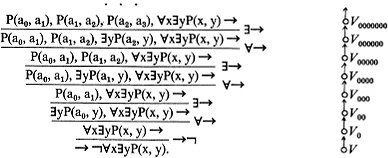
Thus we represent the analysis or search in Example 1 by the following "tree" (left).

We have placed a cross “ × ” at the top of one path or branch to show that this path is (terminated and) closed to us in our search for a counterexample, a check "×" at the top of the other to indicate that the search has terminated successfully there. The symbol "→⊃" indicates that the step in question is an analysis of an implication in the succedent (which we are aiming to make f), "∃→" that it is an analysis of an existence formula in the antecedent (which we are aiming to make t), etc.

The tree of sequents (left) can be considered as the result of placing sequents on the vertices of a purely geometric tree (shown without the sequents at the right). The geometric tree in this example consists of 7 vertices in a certain arrangement (a "partial ordering") shown by the arrows. Thus, the sequent Q(a₀), P →∀xQ(x) is placed at the vertex V₀₀₀₁. A path or "avenue" in our search for a counterexample is represented by a succession of vertices, starting at the bottom and following arrows in the tree. There are two paths in this example, VV₀V₀₀V₀₀₀V₀₀₀₀ and VV₀V₀₀V₀₀₀V₀₀₀₁V₀₀₀₁₀; they run together as far as the vertex K₀₀₀, after which they diverge.224

EXAMPLE 2. Let F be ∃x(P ⊃ Q(x)) ⊃ (P ⊃ ∃xQ(x)). The analysis is the same as in Example 1, except with ∃xQ(x) in place of ∀xQ(x), down through (8). Now to make (5) ∃xQ(x) f, it is necessary that (9) Q(a₀) be f. This is sufficient if the domain D contains only a₀, but not otherwise. So in representing the new situation we don’t omit ∃xQ(x) from the list of the formulas we are aiming to make f. (We haven’t finally picked D yet; we have thus far only committed ourselves to its having at least the element a₀ introduced at (6).) However, if we look at the situation we now have on the second path (ii), we see that the requirement that (9) Q(a₀) be f conflicts with the requirement that (8) Q(a₀) be t. So in this example both paths or avenues open to us in searching systematically for a counterexample to F are closed, or the tree itself is closed. This completes an informal proof (in a classical observer’s language) that there is no counterexample to this F, i.e. a proof that F is valid. Now it would be surprising if we could not utilize the method of this informal proof that F to construct a formal proof of the formula F and thus to show that 1- F. If our formal system of predicate calculus in Chapter II were not adequate to do this, we would certainly look for ways to augment it. However, we postpone this part of the problem to § 51. The sequent tree in this Example 2 is as follows. (Several formulas are in boldface for later reference.)

Before continuing, we observe that we can codify the steps of analysis we are using in our searches. In terms of the representation by trees of

sequents, each step is performable by one of the following 14 rules. Thus, we have several times used the principle that, in order to make an implication A ⊃ B f, it is necessary and sufficient to make A t and B f. This is now codified by the rule at the upper left, called "→⊃" or "the ⊃-succedent rule". The T and 0 tag along to indicate lists of zero or more formulas not changed in the step, those in T to be made t and those in 0 to be made f.

In these rules, A and B are (allowed to be) any formulas; x is any variable; A(x) is any formula; b is any variable free for x in A(x) (and unless b is x not occurring free in A(x)); r is any variable not necessarily distinct from the other variables present, or (if formation rules as in § 28 are used) any term, free for x in A(x); A(b) and A(r) are the results of substituting b and r respectively for the free occurrences of x in A(x); and Γ and Θ are any (finite) lists of (zero or more) formulas.

In using the rules →∀ and ∃→, we must obey the restriction on variables (stated with the rules); briefly, b shall not occur free in the sequent below the line. (When the A(x) does not contain the x free, then A(b) is A(x) no matter what variable b is. We agree in such a case to

choose for the analysis a variable b not occurring free in the lower sequent, so the restriction will be met.)

The order of listing the formulas within any antecedent and within any succedent is to be immaterial in applying the rules. Thus in Examples 1 and 2, the rule ∃→(bottom right) applies from V₀₀ to V₀₀₀ (with a₀ as the b), even though ∃x(P ⊃ Q(x)) is not written first in the antecedent.

Let us extend our evaluation process from formulas to sequents, thus: Δ→λ shall take the value f when all of Δ are t and all of λ are f; otherwise, the value t. We say a sequent Δ→λ is falsifiable, if for some (non-empty) domain D and some assignment in D to (at least) all its parameters, it takes the value f. We say Δ →λ is valid, or in symbols Δ→λ, in contrary case that, for every (non-empty) domain and assignment,Δ→λ is t.

Each of the 14 rules has been picked (by reasoning illustrated in Examples 1 and 2, (a) for necessity and (b) for sufficiency) to have the property stated in:

LEMMA 6. For each of the 14 rules →⊃,..., ∃→listed above, with the stated stipulations: The sequent written below the line is falsifiable, (b) if and (a) only if the sequent, or at least one of the two sequents, written above the line is falsifiable. Equivalently: The sequent written below the line is valid, (a) if and (b) only if the sequent, or each of the two sequents, written above the line is valid.

It is of course quicker to use the rules than to think through the principles embodied in them at each step.

Proceeding upward, we can close a path (signifying that we have lost hope of finding a counterexample along it) when we have reached a sequent which we recognize cannot be made f. We codify this by saying we shall close a path as soon as we reach a sequent of the form

Here we could allow C to be any formula. However it will be useful later (in §§ 55, 56) to know that mistaken attempts at counterexamples can always be rejected using an atom (prime formula) as the C. So we stipulate here that C be such. As with the rules, Γ and Θ are any lists of formulas; and the order of formulas within the antecedent and within the succedent is immaterial.

LEMMA 7. No sequent of the form (x) is falsifiable. Equivalently: Each sequent of the form (x) is valid.

Example 1 illustrates the situation envisaged in (I) of our proposed

plan of attack on the completeness problem (tenth paragraph of this section). Example 2 illustrates (II), provided we can convert the closed sequent tree into a formal proof of F. We give three more examples.

EXAMPLE 3.

Here there is a single path (no branching). This path can be pursued upward ad infinitum: along it we never reach either a sequent of the form (x) at which we can close it (as at V₀₀₀₀ in Example 1, and at both V₀₀₀₀ and F₀₀₀₁₀ in Example 2), or a sequent from which no further step upward can be made by our rules (as at V₀₀₀₁₀ in Example 1). Does this tree lead us to a counterexample?

Indeed it does, under either of two approaches. At V₀₀₀, we know that to falsify ¬∀x∃yP(x, y) it is (necessary and) sufficient to make P(a₀, a₁ and ∀x∃yP(x, y) both t. There are two possibilities: a₀ and a₁ are the same element of the domain D, or different elements. Under the first approach, we try making D = {0} with 0 as the value of both a₀ and a₁. We evaluate P by the logical function I for which I(0, 0) is t, so P(a₀, a₁) is t. Evidently this also makes ∀x∃yP(x, y) t; or we can argue that for a D with only the element a₀ we could have omitted ∀x∃P(x, y) at V₀₀ and hence at V₀₀₀. Thus we have a counterexample, indicated by the tree just up to V₀₀₀.

Now let us instead try having a₀ and a₁ different elements of D, and (following this approach consistently) likewise having each of a₂, a₃, a₄,. .. in turn a new element. Let D = {0, 1, 2,...}, and assign to a₀, a₁, a₂,... the values 0, 1, 2,.... To P let us assign the logical function I such that I(x, y) is t when x and y are consecutive natural numbers, and always f (or always t) otherwise. This makes all the atoms in the antecedents t. The student should have no trouble in seeing that consequently it makes also the molecules there t, and hence makes ¬∀x∃yP(x, y) in the succedent at the bottom f. So we have another counterexample, corresponding to the whole infinite path.

Let us consider the two approaches in general.225 When we try for a counterexample, at each step upward by →∀ or ∃→ we have a choice between the two for the variable b introduced in that step if any variables were previously introduced (as at (9) or V₀₀₀₁₀ in Example 1, and at V₀₀₀ in Example 3, with a₁ as the b). Suppose there is a counterexample using the first approach, i.e. with b standing for the same element of D as some other variable a already introduced (as a₀ in Example 3). Then there is also a counterexample using the second approach. We can get this from the first counterexample by splitting the element represented by both a and b into two elements (enlarging D by one element) and treating these two elements (one to be used as value of a and the other of b) like the one element they replace in constructing the logical functions (and functions with values in D if mesons are present) for the falsifying assignment.²²⁶ (As we have seen, in Example 3 at V₀₀₀ both approaches work; in Example 1 at V₀₀₀₁₀ only the second works.) So we can never miss finding a counterexample (if a counterexample exists at all) by confining ourselves to the second approach. The treatment in §§ 49, 50 is set up on this basis. In it, we will provide for terminating a path in a sequent tree (even though the rules could be applied further) when a stage is reached from which a counterexample can be read off under the second approach. For our primary purpose of proving GödePs completeness theorem, the additional possibilities for finding counterexamples afforded by the first approach are an unnecessary distraction. Of course, the first approach will often lead to a counterexample more quickly or to a simpler counterexample (as in Example 3).

In Example 3, using the second approach, we saw how an infinite counterexample (i.e. one with an infinite D) can be read off a suitably constructed infinite path. In Example 3, there was also a finite counterexample, using the first approach. Our last two examples will illustrate two points: (a) there may be only infinite counterexamples (Example 4); (b) without some over-all plan governing our searches, they may not lead to a counterexample or a closed tree, even though there be one or the other (Examples 4 and 5).

EXAMPLE 4. Let G be

The tree shown is to be continued upward ad infinitum from V₀₀ with the same sequents as in Example 3 from V₀ except that G is at the front of each antecedent.

The one path in this tree does not indicate to us a counterexample. For, in building it upward as proposed, we spend forever analyzing the conditions for the truth of ∀x∃yP(x, y) (as in Example 3) and never get to those for G.

Now we show that there is a counterexample to ¬(G & ∀x∃yP(x, y)) with D = {0, 1, 2, ... } but no finite counterexample.

To do this it will suffice to show that G & ∀x∃yP(x, y) is t for a suitable assignment in D = {0, 1, 2, . ..}, but is always f in any finite (nonempty) domain.

It is easy to see what is going on, if in G & ∀x∃yP(x, y) we not only unabbreviate G, but take the outer conjunctions apart, omit the universal quantifiers, and change P(—, —) to —<—:

These order axioms are all true (with the free variables in the generality interpretation, §§ 20, 38) when D = {0, 1, 2, . . .} and < stands for the usual order relation between natural numbers. Thus G & ∀x∃yP(x, y) is t(and -i(G & ∀x∃yP(x, y) is f), when D = {0, 1, 2, . . .} and to P is assigned as value the logical function I such that I(x, y) is t when x<y and f otherwise.

But these order axioms cannot be satisfied in any finite (non-empty) domain, as we now show. Consider e.g. a domain D with just three elements. Say one of the elements is a₀. By ∃y x<y, there is some y such that a₀<y; by ¬x<x this y cannot be a₀; say it is a₁ (different from a₀); thus a₀<a₁. Again using ∃y x<y, there is a y such that a₁<y; by ¬x<x this cannot be a₁; and also it cannot be a₀, since then a₀<a₁ and a₁<a₀ with x<y&y<z⊃x<z would give a₀<a₀, contradicting ¬x<x; so this y is the remaining element a₂; thus a₁<a₂. Now by ∃y x<y, there must

be a y such that a₂<y; but in the manner already illustrated, this y cannot be a₀ or a₁ or a₂. So it is impossible to have all three formulas written with < true simultaneously, if D has just three elements. If we construct the truth table for G& ∀x∃yP(x,y) with D = {0, 1, 2} in the manner of § 17 (it will have 2⁹ = 512 lines), we shall get a solid column of f’s. The like will be the case for every finite (non-empty) D (i.e. for D = 1, 2, 3, .. .)

The fact that there are formulas which are valid (not falsifiable) in every non-empty finite domain, but are not valid (are falsifiable) in D = {0, 1, 2,...}, was first noticed by Löwenheim 1915; the present example ¬(G & ∀x∃yP(x, y)) is from Hilbert and Bernays 1934 pp. 123-124.

We shall not take the space now to illustrate how our search procedure, when suitably managed (differently than above), leads to a counterexample in Example 4 (Exercise 49.3).

EXAMPLE 5. Take the tree as in Example 4, but with Q & ¬Q as the G. There is no counterexample (since at V₀₀ we can’t make G t). But as we are misconducting the search, this doesn’t manifest itself by the path becoming closed.

From Example 4 (and Example 3 if we confine ourselves to the second approach) we see that we must interpret (I) broadly enough to include counterexamples that are only developed by pursuing the search along some path ad infinitum. But our aim is to show for (II) that, in a properly managed search, if no counterexample exists (F is valid), that fact will always manifest itself by the closing of all paths after a finite amount of searching (as in Example 2). This is why, when F is valid, we shall always be able to find a proof of F (§ 51).

We could have anticipated from Theorem VII of Church that, if under (II) we are always to have a finite closed tree, then under (I) we cannot always effectively learn the existence of a counterexample in finitely many steps, whatever procedure we adopt. For, if we could, then we would have an algorithm or decision procedure (§ 40) for answering all questions whether a formula F in the predicate calculus is valid. By GödeFs completeness theorem (which we are aiming to prove) with Theorem 12_Pd (§ 23), this would be an algorithm for provability in the predicate calculus, contradicting Theorem VII.²²⁷

This situation is the reverse of what we might naively have expected back in § 17, where we found some finite counterexamples, but required general reasoning to establish validity.

In Example 3 (with the second approach) and Example 4, although the counterexamples are infinite, the logical functions or predicates can be described effectively ;¹⁶⁴ i.e. there are algorithms for them. This will not always happen under (I).²²⁸

EXERCISES. 48.1. By a systematic search (presented as a sequent tree), either find (and describe) a counterexample, or show that there is none. (a)P∨Q⊃P&Q. (b) (P ⊃¬P) ⊃¬P. (c) P ∨ ∀xQ(x) ⊃ ∀x(P ∨ Q(x)). (d) ∃xP(x) & ∃xQ(x) ⊃ ∃x(P(x) & Q(x)).

48.2. Show that (under the definition preceding Lemma 6): (a) A_l.. ., A_m → B_l, .., B_n, if and only if, for each (non-empty) domain D and each assignment in D to the parameters of A₁,..., A_m → B₁,..., B_n, .either m > 0 and one of A_l, .. ., A_m is f, or n > 0 and one of B_l, ... ., B_n is t (briefly: either some of A_l..., A_m are f, or some of B_l..., B_n are t; cf. § 26). (b) Hence: A_l. . ., A_m → B if and only if A₁,..., A_m B (§20).

48.3*. Using insight (as in Example 4) rather than the systematic search procedure, find a counterexample in D = {0, 1, 2,...} to

Show that there is no finite counterexample.

§49. Gödel’s completeness theorem: the basic discovery.

Examples 4 and 5 have shown that we must adopt some over-all plan to guide our systematic searches for counterexamples to formulas F, if we are always to obtain either a counterexample or a closed tree.

The forms of the individual analytical steps upward have been described adequately by the list of 14 rules. Prior to adopting a search plan, we shall note some features of the steps (or the rules for them).

In each step upward by one of the rules, we recopy the list of formulas we are aiming to make t and the list we are aiming to make f, with a revision or two alternative revisions. The revision comes from analyzing the conditions for the truth t or the falsity f of one of the formulas (the principal formula in the step) with respect to its outermost propositional connective or quantifier (the principal operator). On the basis of this analysis, we introduce into our lists one or two other formulas (the side formula(s)). Thereupon the principal formula becomes redundant and is omitted, except in the two rules ∀→ and →∃. The remaining formulas

(extra formulas) are recopied unchanged. For example:

Hence in an obvious way, when we make a step upward by one of the rules, each formula occurrence (as one of the formulas listed as the antecedent or as the succedent) in the sequent or in either sequent above the line “originates from” or belongs to or is an (immediate) ancestor of a particular formula occurrence in the sequent below the line (its immediate descendant). ’Here we assume that, in any case of doubt, an analysis has been adopted fixing which formula occurrence is the principal formula, which are the side formula or respective side formulas, and which extra formula occurrence above comes from each one below.229

We can trace these ancestral relationships upward (or descendant relationships downward) through a succession of steps. Also, besides the ancestors of a formula occurrence in sequents above its own (proper ancestors), it is convenient to consider it as its own ancestor in its own sequent (its improper ancestor); and likewise with descendants. To illustrate this, in Example 2 all 6 ancestors of the formula (occurrence) in the antecedent at V₀ are printed with letters in boldface.

Like relationships apply to formula parts of formulas, to operator occurrences in formulas, and to occurrences of predicate parameters. In Example 2, the first ⊃ in the bottom sequent has four ancestors, namely itself and the three ⊃’s in boldface formulas; the first Q has 6 ancestors, itself and the 5.boldface Q’s.

In designating these relationships for formula parts (or wholes) of formulas, we use image (or ancestral image and descendant image) instead of “ancestor” or “descendant” when we wish to restrict the relationship to parts (or wholes) which are the same except possibly for substitutions of terms for variables (reading up) or inversely (reading down). Thus in Example 2 reading down, the boldface Q(a₀) at F₀₀₀₁₀ has as (descendant) images Q(a₀), Q(a₀), Q(a₀), Q(x), Q(x), Q(x), and as descendants Q(a₀),

Q(a₀), P⊃Q(a₀),∃x(P⊃Q(x)), ∃x(P⊃Q(x)), ∃x(P ⊃ Q(x)) ⊃(P⊃∃xQ(x)). Reading up, P ∃ Q(x) at V has as (ancestral) images P ⊃ Q(x), P ⊃ Q(x), P ⊃ Q(x), P ⊃ Q(a₀). For operator or predicate parameter occurrences, “ancestral image” and “descendant image” are synonymous with “ancestor” and “descendant”, respectively.

A given composite formula occurrence in a sequent can serve as the principal formula for only one of the 14 (= 2·7) rules, according as the occurrence is in the succedent or the antecedent (2 choices) and according to the kind of the operator which it has outermost (7 choices). So we can classify the composite formula occurrences in sequents by the rules applicable to them as principal formulas.

In treating the problem of falsifying a formula F via our search procedure, the problem quickly generalized itself to that of simultaneously making m formulas A_l. .., A_m t and n formulas B₁,... ., B_n f, or equivalently (by the definition preceding Lemma 6) of making a sequent A₁,... ., A_m →; B₁,. . ., B_n f (m,n> 0). In other words, A_l. . ., A_m are to be satisfied and B₁..., B_n to be falsified, simultaneously; or A_l. . ., A_m → B_l. .., B_n is to be falsified.

Now we are ready to adopt a plan to guide our systematic searches for counterexamples.

First (Case (A)), we undertake to falsify a sequent

E₁,....E_k → F_l. . ., F_l where E_l.. ., E_k, F_l, .., F_l are formulas in the sense of § 16, except that they may contain individual symbols (but not other function symbols).²³⁰ By taking → F as the sequent, this includes the case of falsifying a single formula F. The sequent E_l.. ., E_k → F_l. . ., F_l may contain free variables, but those variables shall not also occur bound in it.²³¹

Let u₀,.. ., u_p be a list (possibly empty) of the free variables and individual symbols occurring in E₁.. ., E_k → F_l.. ., F_l. Let a₀, a_l a₂, . .. be variables not occurring in E₁ .. ., E_k → F_l. . ., F_l. The terms u₀,. . ., u_p, a₀, a_l a₂,. . ., as far as we activate them (i.e. make them available), will be used as the b’s and r’s for our applications of the predicate rules →∀, ∀→, →∃, ∃→. Because the variables among u₀,. . ., U_p do not occur bound in E_l..., E_k → F_l. .., F_l and a₀, a_l a₂, ... are "new" variables not occurring in E₁. . ., E_k → F_l.. ., F_l the substitutions with results A(b) and A(r) performed in using these rules

will be free.232 Those of u₀,. . ., u_p a₀, a_l a₂, ... which we activate are intended to name distinct members of the domain D for the counterexample to E_l. . ., E_k →F_l..., F_l we are attempting to construct.²³³ As the search for a counterexample to E_l.. . ,E_k→F_l. . . F_l is pursued along any particular path in our sequent tree, we keep track step by step of which of u₀,. . ., u_p, a₀, a₁ a₂,. . . have thus far been activated. To represent this concretely, we may employ a barrier |. We put the barrier into the list initially just to the right of _p, thus,

to indicate that u₀,..., u_p are activated initially, if u₀,.. ., u_p, is not empty. But if u₀,. .., u_p, is empty, we place the barrier initially thus,

to indicate that in that case a₀ is activated initially. In each step by →∀ or ∃→, we shall use a new variable as the b. Suppose that thus far u₀,..., u_p a₀,. .., a_i-1 or briefly t₀,.. ., t_Q (q = p+i+1) have been activated, so the list looks so:

As the b for the →∀ or ∃→, we then use a_i, at the same time moving the barrier over to indicate that this variable is added to the part of the list which has been activated:

The steps along any particular path of the tree will be grouped in rounds.

Say that at the beginning of a certain round, call it Round d₉ we have before us a sequent Δ → A or more explicitly A_l. .., A_m → B₁..., B_n. (For d = 0, this is E_l.. ., E_k. →F_l. .., F_l. For d > 0, it is the sequent reached at the end of Round d-1.)

In carrying out Round d, we take each of the formula occurrences A_l..., A_m, B_l..., B_n in turn (or more precisely, after the first step, a proper ancestral image of that formula occurrence), and perform if possible one step or a finite number of steps with it as principal formula (unless part way through the round we close the path, as explained below).

No step can be performed in case the one of A₁,.. ., A_m, B₁,.. ., B_n in question is an atom.

In the case of a formula occurrence of one of the kinds →⊃,..., ~→;, one step is performed, which is completely determined by the formula and the corresponding rule.

In the case of a formula occurrence of one of the kinds →∀, ∃→, one step is performed by the respective rule, with the next variable a, after those previously activated as the b (as explained above).

In the case of a formula occurrence of one of the kinds ∀→,→∃ steps are performed by the respective rule using as the r each one in turn of the terms t₀,.. ., t_Q already activated which has not previously served as the r for that rule with the same principal formula (or more precisely, with a descendant image of it as the principal formula). This calls for from 0 to q+l steps.

A particular path will be terminated and closed exactly when a sequent is first reached of the form (x) with C prime, disregarding as usual the order of formulas within antecedent and within succedent.

A path will be terminated without being closed exactly when a sequent is reached from which no step as prescribed is possible. This will happen at a given sequent (with t₀,..., t_Q the terms thus far activated) exactly when the sequent contains only atoms, and ∀→- and →∃-formulas descendant images of which have already served as the principal formula with each of t₀,..., t_q as the r. (This can only happen at the end of a round, in which case there is no next round.)

We can summarize our search plan thus. We provide for a non-empty domain D by activating u₀, . . . , u_p, or a₀ initially. In each round, we go through the double list of formula occurrences A₁ . . ., A_m, B_l .. . , B_n reached at the end of the preceding round (or given initially), analyzing each molecule in turn, with respect to its outermost operator only (with the terms t₀,. . ., t_q thus far activated as the r’s for ∀→ and →∃), before starting over at the beginning of the list in the next round.

LEMMA 8. In a sequent tree constructed upward from E₁. . ., E_k → F₁... , F_l using the 14 rules and the described search plan, consider any unclosed path, terminated or infinite. The list t₀,. . . , t_Q or t₀ t_lt₂,. . . of the terms which are eventually "activated" along the path is not empty, and includes all the individual parameters of E_l. . ., E_k → F_l.. ., F_l and all the terms used as b’s and r’s for →∀, ∀→, →∃, ∃→ along the path, and hence every individual parameter of any sequent along the path.^2U Each molecule occurring (in the antecedent or

the succedent) in any sequent along the path is used as principal formula (in the antecedent or succedent respectively) somewhere along the path, namely, just once, except in the case of an ∀→- or →∃-molecule, which is so used with each of t₀,..., t_q or t₀, t_l t₂, . . . as the r.

PROFF. For a molecule occurrence not of the kind ∀→ or →∃ ,an ancestral image of it will be used as principal formula during the next round after the one in which the formula first appears (or in the case of one of E_l..., E_k, F_l..., F_l in the first round). An ∀→- or →∃-formula occurrence, once it has appeared, will never disappear. An ancestral image of it will be called up for use as principal formula, with every activated term not yet used as the r, in every subsequent round (and in the first round, if it is one of E₁, . .., E_k, F_l ..., F_l), either ad infinitum or until the path is terminated. The path can be terminated only when all activated terms have served thus as the r. —

We picked the particular search plan described above to get Lemma 8 quickly, toward proving GödePs completeness theorem. In practice, the search for a counterexample to E₁,.. . ,E_k→F₁,. .. ,F_l can often be conducted more efficiently (without sacrificing Lemma 8) by allowing some variation from the above plan. Examples 1 and 2 take a little longer to complete under the above plan than in §48 (Exercise 49.1 (a) and (b)).²³⁵

LEMMA 9. In a sequent tree constructed upward from

E_l. .., E_k → F_l. .., F_l using the 14 rules and the described search plan, corresponding to any unclosed path, terminated or infinite, there is a counterexample to E_l . . ., E_k → F_l . . ., F_l with the domain D = {0,. . ., q} or D = {0, 1,2,...} according as only t₀,. . ., t_Q or t₀, t_lt₂, . . . are activated along the path.

PROOF. Let the sequents along such a path be Δ₀ → λ₀,..., Δ_t→ λ_t (terminated unclosed path) or Δ₀ → λ₀, Δ₁ → λ_l, Δ₂ → λ₂, .. . (infinite path), where Δ₀ → λ₀ is E₁,. .., E_k → F_l..., F_l. Let ∪ Δ be the set of all the formulas which occur in any of the antecedents Δ₀,. .., Δ_t or Δ₀,

Δ_l ,Δ₂,..., and similarly let ∪A be the union of all the λ’s. We shall show that, with the domain D as described, we can pick an assignment in D to make all the formulas in ∪Δ (including E_l,..., E_k) t and all those in ∪λ (including F₁ ..., F_l) f.236

Because the path is not closed, ∪Δ and ∪λ contain no atom C in common. For, suppose they did; say C first enters the antecedents in Δ_a and first enters the succedents in λ_b. Once an atom has entered an antecedent or succedent, it rides up into all higher sequents in antecedent or succedent respectively in the extra formulas Γ or Θ of the steps. So C would be in both Δ_c and λ_c where c = max(a, b) (the greater of a and b, or their common value). So the path would have been terminated and closed (by use of (x)) at Δ_c → λ_c (if not before).

It will follow that, with the domain D as described in the lemma, we can pick an assignment to (at least) all the parameters of ∪Δ and ∪λ which makes all atoms in ∪Δ t and all in ∪λ f. As the parameters, we take (a) the variables and individual symbols t₀,.. ., t_q or t₀, t_l,t₂,..., (b) the proposition symbols occurring in ∪Δ or ∪λ, and (c) the other predicate symbols so occurring. We take D = {0,..., q) or D = {0, 1, 2,...} respectively, and we assign to t₀,..., t_q the values 0,..., q, or to t₀, t_1} t₂,... the values 0, 1, 2, .... To each of (b) we assign t if that proposition atom occurs in ∪Δ, f it occurs in ∪λ (we have seen that it can’t occur in both), and an arbitrary value say f if it occurs in neither. To each of (c) we assign the logical function I such that I(x_l..., x_n) is t if the predicate atom P(t_a.₁,. .., t_an) occurs in ∪Δ, f if P(t_a._i,. . ., t^) occurs in ∪λ (it can’t occur in both), and say f if it occurs in neither.⁶⁴ Each predicate atom in ∪Δ or ∪λ is of the form P(t_x1 ,. . ., t_xn ) for some x_l. . ., x_n belonging to D, using the second sentence of Lemma 8. Hence, all atoms in ∪ Δ will now be t and all in ∪ λ will be f, as required.

Finally, we show that the D and assignment picked to make all atoms in ∪Δ t and all in ∪λ f also makes all molecules in ∪Δ t and all in ∪λ f. Suppose it did not. Then, from among all the molecules in ∪Δ which are not t or in ∪Δ which are not f, let us choose one G containing the smallest number (> 1) of occurrences of operators. By the last sentence of Lemma 8, G plays the role of principal formula (for the antecedent or succedent rule appropriate to its outermost operator, according as G is picked from ∪Δ or from ∪λ). For G not an ∀→ or →∃-formula, consider the side formula(s) H, or H and I, which are in the premise belonging to the path in question. By the choice of the 14 rules except ∀→ and →∃, the formula(s)

H, or H and I, having the desired value(s) (t in the antecedent, f in the succedent) is sufficient for G to have the desired value. (This property of the rules gave us Lemma 6 (b).) But H, or H and I, having fewer occurrences of operators than G, do have the desired value(s), since G was supposed to have the minimum number of operator occurrences for formulas not having the desired values. So such a G cannot exist, unless it is an ∀→- or →∃-formula, i.e. ∀xA(x) in the antecedent or ∃x A(x) in the succedent. Then by end Lemma 8, A(r) occurs as side formula for each of t₀, . . ., t_q or of t₀, t_l,t₂,. .. as the r. But under our assignment these variables name all the members of the domain D. So G must get the desired value, in consequence of all the side formulas A(t₀), .. ., A(t_q) or A(t₀), A(t₁), A(t₂),... getting the desired values (since they each have one less operator occurrence), contradicting the choice of G. —

In the following lemma dealing with geometric trees, we mean by a partial path a succession of vertices connected by following the arrows, starting with the initial vertex V. (By a path, we have meant such a succession of vertices continued either to termination or ad infinitum.)

LEMMA 10. (König’s lemma 1926.)237 In a geometric tree with finitely many arrows leading from each vertex, if there are arbitrarily long finite partial paths, then there is an infinite path.

PROOF AND ILLUSTRATION. In the application we are to make, the number of arrows leading from a vertex can be 0, 1 or 2. Very simple geometric trees of this kind are shown in Examples 1-4; here is a more complicated such tree (drawn horizontally to save space):

To give the proff in general, suppose we are dealing with a tree as described long partial paths. We wish to trace an infinite path. Here is the rule for doing so. Suppose we have traced the desired path as far as vertex V_x (either the initial vertex V, or a later vertex such as V₁₁₀₀ in the illustration), and that V_x belongs to arbitrarily long finite partial paths (as does V by hypothesis). We want to pick a next vertex that will also have the italicized property. There must be a next vertex after V_X or V_x could not have the property; say the next vertices are V_X0, ... ,V_Xn .One at least of these next vertices must have the property; for if the partial paths through V_X0,..., V_Xn were no longer than b₀,..., b_n vertices respectively, then all partial paths through V_x would be no longer than max(b₀,..., b_n) vertices. So we can indeed pick a next vertex after V_x also having the property. Altogether, starting with V, we are thus able to pick a next vertex, always with the property, ad infinitum.

In the illustration above, if the boldface vertices are the ones which belong to arbitrarily long finite partial paths, then one infinite path (boldface arrows) starts out VV₁V₁₁V₁₁₀V₁₁₀₀V₁₁₀₀₁....

EXAMPLE 6. For trees in which infinitely many arrows may lead from a vertex, the lemma need not hold. Consider the tree in which χ₀ arrows each lead from V to a next vertex V_x (x = 0, 1, 2, ...); and from V_x successive arrows lead to x more vertices V_x0, V_x00 , . . . , thus:

In this tree, there are arbitrarily long finite partial paths, but no infinite path. —

Now, given a sequent E₁, . . ., E_k → F₁, . . ., F_l as specified for Case (A), let us start constructing the sequent tree upward from it, using the 14 rules and the described search plan. The succession of steps along any path is governed by the search plan. Let us divide our work between the different paths, when there is branching, so that different paths are constructed up to corresponding levels in step. Thus, after having constructed up to their 10th vertices all partial paths which don’t terminate sooner, we take each of these which doesn’t terminate at its 10th vertex and add the one or two 11th vertices issuing from it, before we put a 12th vertex on any path.

CASE 1: for some b, each path terminates and closes with not more than b vertices. Then the tree itself is closed, and finite (it has at most 1 + 2 + 2² + . . . + 2^b-1 = 2^b — 1 vertices). So there is no counterexample, i.e. E₁,..., E_k → F₁,..., F_l. (To review the argument, already illustrated by Example 2, at each partial stage in the tree construction, our sole hope of getting a counterexample is that one of the sequents that stand at the tops of branches can be falsified; indeed, we know this by repeated applications of Lemma 6 (a). But with the whole tree closed, each sequent at the top is not falsifiable, by Lemma 7.)

CASE 2: for some b some path terminates unclosed at its bth vertex. Then by Lemma 9, there is a counterexample to E₁,..., E_k → F₁,..., F_l with D = {0,..., q}. (Along a terminated path, only finitely many terms t₀,..., t_q can be activated in this Case (A).)

CASE 3: otherwise. Then the tree has arbitrarily long finite partial paths. So by Kösnig’s lemma (Lemma 10), there is an infinite path. Hence by Lemma 9, there is a counterexample with D = {0,..., q} or D = {0, 1, 2, ...}.²³⁴

We have now reached our goal for this section. To simplify the statement (italicized next below), we can take D = {0, 1, 2,...} in both Cases 2 and 3. For, if there is a finite counterexample, we can manufacture a countably infinite one from it by splitting an element into χ₀ elements, all behaving like the original element in the evaluation process. (We used this idea, splitting an element into 2, in §§ 30, 48.)

PRELIMINARY VERSION OF THEOREMS 33 AND 34°. For a sequent E₁, . . ., E_k → F₁, . . ., F_l as described for Case (A) (containing no variables both free and bound): Either (I) there is a counterexample to E₁, . . ., E_k → F₁, . . ., F_l in the domain {0, 1, 2, . . .}, or (II) there is a (finite) closed sequent tree constructed upward from E₁, . . ., E_k → F₁. . ., F_l by the 14 rules, and hence there is no counterexample to E₁,..., E_k → F₁,..., F_l i.e. E₁,..., E_k → F₁,..., F_l.

It follows as a side result that E₁,..., E_k → F₁,..., F_l cannot have uncountably infinite counterexamples and no others:

PRELIMINARY VERSION OF THEOREM 35. For a sequent E₁,..., E_k →F₁,..., F_l as described for Case (A): If there is any counterexample to E₁,..., E_k →F₁,..., F_l, then there is one in the domain {0,1,2,...}.

EXERCISES. 49.1. Construct the sequent tree upward (using the described search plan), and conclude (1) (give .the counterexample) or (II):

49.2. Apply the search plan to and . Why does it fail for the latter?

49.3*. Consider making a systematic search for a counterexample to (Example 4 § 48), by using the 14 rules upward with the following search plan (different from the plan in the text): in Round 0, perform all steps possible with only a₀ activated; in Round 1, activate a₁ by ∃→ and then perform all new steps possible with only a₀, a₁ activated; in Round 2, activate a₂ by ∃→ and then perform all new steps possible with only a₀, a₁ a₂ activated; etc.

(a) Show that Lemma 8 is satisfied by this search plan.

(b) Show that, if the steps are continued to the end of Round d suspending the rule for closing paths, there will be 3(d+l)³ “branches” or partial paths. (Thus, activating only a₀, a₁ a₂ as in the informal discussion in Example 4, there will be 81 paths, if the possibilities for closing some of those paths before completing all the disections are disregarded.)

(c) Using as a guide the counterexample which we found by insight in Example 4, pick at each branching the sequent along a path which goes with that counterexample. Write the sequent which will be reached at the end of Round 1 along the resulting infinite path.

§ 50. Gödel’s completeness theorem with a Gentzen-type formal system, the Löwenheim-Skolem theorem. Now we would have the first case of Gödel’s 1930 completeness theorem (If F, then F), if under (II) just above (for k = 0, l = 1) we could infer that F in the sense of § 21. (We shall do so in § 51.)

However, we already have the basic discovery. This is that, whenever no counterexample to F exists (i.e. when F), that fact can be confirmed by a finite mechanical verification process.²³⁸ This process (in the present treatment) consists in verifying that a certain finite figure meets the conditions for being a closed sequent tree constructed upward from → F using the 14 rules.

From the standpoint from which formal systems and proof theory were invented (§ 37), this fundamentally is all we were after. We could take the mechanical verification process as itself constituting a proof of F.

In fact, these verifications come under essentially the traditional form for axiomatic-deductive systems, if we simply read downward in checking the correctness of the trees, instead of upward. At the top of each branch, if the tree is closed, we have a sequent fitting (×) in § 48, which we can now consider to be an axiom schema. (Now “×” instead of meaning “closed” can mean “axiom”.) And each step downward is by one of 14 rules (previously read upward), which we can now regard as one- or two-premise rules of inference. (Now “⊃→” can be called “⊃-introduction in the antecedent”, etc.)

Now any tree with axioms by (×) at the tops of branches, and each step downward by one of the 14 rules, constitutes a proof {of its bottom sequent or endsequent) in a formal system G4 of a new type, called a Gentzen-type (sequent) system or sequent calculus. ²³⁹ Such systems were introduced by Gentzen 1934-5 (and 1932), in part following Hertz 1929. In contrast, we call the formal system for the predicate calculus of § 21 a Hilbert-type system H. More precisely, “G4” and “H” denote ambiguously several systems, according to how the notions of term and formula (specifically, of prime formula) are regulated (cf. §§ 37, 39).

By Lemmas 6 (a) and 7, G4 has the consistency property analogous to Theorem 12_Pd for H:

THEOREM 33. Each sequent A₁,..., A_m → B₁,..., B_n provable in G4 is valid; in symbols, if A₁,..., A_m → B₁,..., B_n, then A₁,...,A_m → B₁,...,B_n.

This is only a restatement of the feature of our searches that closure of the tree means that all possibilities for finding a counterexample have been closed out. Without this consistency property, we would hardly want to use G4 as a formal system.

Lemma 6(b) expresses a novel property of (the rules in) G4, not possessed in H by the rule of modus ponens.²⁴⁰

The fact that G4 operates with sequents, so → F (rather than F) is provable in G4 when the search procedure closes, is not a serious drawback. Anyone who objects to this could easily modify G4 to use formulas as did Schütte 1950 (though the sequents are convenient), or he could supplement G4 by a rule → F / F.

Also G4 has the new feature that its proofs are finite trees (they are “proofs in tree form”) rather than finite (linear) sequences of formulas (“proofs in sequence form”). We could rewrite the trees in sequence form.

But the trees show the logical structure better, and thus help us in our reasoning about that structure. The linear arrangement of proofs has been traditional, no doubt because oral language is necessarily linear, and written language more conveniently so for ordinary purposes. Proofs (and deductions) in H can be written in tree form.241

Now we take up some other cases of Gödel’s completeness theorem.

We begin (CASE (B)) by extending the treatment of Case (A) to deal with a countable infinity of formulas ..., E₂, E₁, E₀ to be made t and a countable infinity F₀, F₁, F₂, ... to be made , simultaneously, in which altogether there occur only a finite list u₀,..., u_p (possibly empty) of free variables and individual symbols (but no other function symbols). Such free variables shall not occur bound in any of the formulas. Alternatively, one of the two lists of formulas may be finite or even empty.²⁴² For those alternatives, slight alterations of our notation are to be imagined.²⁴³

To deal with this case, we generalize our notion of sequents and related notions to allow χ₀ formulas in the antecedent and succedent (or in one of them). We now work with the χ₀-sequent ..., E₂, E₁, E₀ → F₀, F₁, F₂,. . . instead of with the sequent E₁,..., E_k → F₁,..., F_l ²⁴⁴.

However, during Round d along any particular path in the tree only the first d +1 formulas of the original lists will have been activated. Say that

is the χ₀-sequent reached at the end of Round d— 1 (or when d = 0, the initial χ₀-sequent, with A₁, . . . , A_m and B₁, . . ., B_n both empty). Then we commence Round d by first moving out the two barriers in the χ₀-sequent before us to activate E_d and F_d, thus,

Then each of E_d, A₁,..., A_m, B₁,..., B_n, F_d in turn is used to the extent possible as principal formula (as A₁,..., A_m, B₁,. . ., B_n were in Case (A)). The criterion for closing a path is that the part of the χ₀-sequent between the barriers (which is a sequent) fit the axiom schema (×), i.e. have an atom common to its antecedent and succedent. After any round with the path not closed, there is always a next round in which at least the barriers are moved one position out. If the formulas E_d and F_d newly activated are atoms, it can happen that there are no steps in that round (i.e. no sequent(s) are added to the tree); namely, this will happen if the sequent previously between the barriers qualified for termination under Case (A). If, in this case, all the formulas outside the barriers are atoms, then termination without closure will take place by having an infinity of rounds happen “instantaneously” (the barriers being simply moved out, one position after another). This is the only way termination without closure can take place. Closure, if it takes place, occurs in some finite round.

No change is required in LEMMAS 8 and 9 other than replacing “sequent” by “χ₀-sequent” and “E₁. . ., E_k → F₁,. . ., F_l” by “..., E₂, E₁ E₀ → F₀, F₁, F₂,...” (and LEMMA 10 does not depend on the case). But in conclusion, if we obtain a closed χ₀-sequent tree, then from it we can obtain a closed sequent tree as follows. Since the χ₀-sequent tree is closed, it is finite (as argued in Case 1 end §49). Consider its finitely many top vertices, and let d be the greatest round during which any of them become closed. Then nowhere in the tree do the two barriers stand further out than just right of (an ancestral image of) E_d+1 in antecedent and just left of F_d+1 in succedent. The pairs of atoms C in top χ₀-sequents which occasion their closure are within the barriers. So are the principal and side formulas in each step. Now let us move the barriers out in every χ₀-sequent up to but not across E_d+1 and F_d+1, and then throw away all formulas still outside the barriers. The result is a closed sequent tree with E_d,..., E₀ → F₀,..., F_d at the bottom.

Finally, we take the cases not already treated of finitely many formulas E₁,..., E_k, F₁,..., F_l, (CASE (C)), or χ₀ formulas . . ., E₂, E₁, E₀, F₀, F₁, F₂,... (CASE (D)), which in the aggregate contain (i) finitely or infinitely many free variables (which shall not also occur in any of the formulas bound) and individual symbols and (ii) finitely or infinitely many other function symbols.245 We write out the treatment supposing there are at least one each of the symbols (i) and (ii). Otherwise, slight modifications are to be imagined.²⁴⁶

To deal with these cases, we prepare χ₀ separate lists of χ₀ terms each, which we show with the initial position of the barrier in each:

The first list u₀, u₁, u₂,... is an enumeration of all the terms (§§ 28, 38, 39) constructible using the symbols (i) and (ii). We can always get an enumeration of the terms thus constructible, e.g. by the method of digits ((A) in § 32). For example, if the formulas contain no free variables but exactly one individual symbol e and two other function symbols f(—) and g(—, —), the enumeration could start out thus:

e, f(e), g(e, e), f(f(e)), f(g(e, e)), g(e, f(e)), g(f(e), e),....

Each subsequent list u_i0, u_i1, u_i2, ... is an enumeration of the additional terms which are constructible when the variable a_i is also made available. Thus u_i0, u_i1, u_i2, ... is an enumeration of the terms constructible allowing the use of the same symbols as for u₀, u₁, u₂,... and the variables a₀,..., a_i and actually using a_i (so we don’t include any terms from earlier lists). For example, if the symbols for u₀, u₁, u₂, . . . are as above, u₁₀, u₁₁, u₁₂,... could start out

a₁, f(a₁), g(a₀, a₁), g(a₁ a₀), g(a₁, a₁), f(f(a₁)), f(g(a₀, a₁)),....

When a step by →∀ or ∃→ is performed, we use as the b the first one a_i of a₀, a₁, a₂, ... not yet activated, and we move the barrier over one place in the list u_i0, u_i1, u_i2,. . . which it begins to record this. In ∀→-and →∃-steps, all the terms t₀,. . . , t_q thus far activated in any of the separate lists are available as the r. The rounds are managed as under Case (A) or (B), except that, after the end of any round at the commencement of the next, we move the barrier one place to the right in each of the lists of terms in which the barrier is not at the extreme left. Thus, along any path in the tree which does not close, once any term in a list is activated, we eventually activate every term in the list; they all go into the consolidated list t₀, t₁ t₂, . . . of all the terms eventually activated. This will happen even in a terminated but unclosed path, by infinitely many rounds being performed “instantaneously” by just moving barriers over in the lists of terms and for Case (D) also in the lists of formulas.

The second sentence of LEMMA 8 now reads: The list t₀, t₁, t₂,... of the terms which are activated along the path is an enumeration of all the terms constructible using the individual and other function parameters of E₁, . . ., E_k → F₁, ..., F_l or of. . . ., E₂, E₁, E₀ → F₀, F₁, F₂,. . . and those of the new variables a₀, a₁, a₂,... which are introduced in using →∀ and ∃→; every r for ∀→ or →∃ is taken from the list; and hence every term occurring free (§ 28) in any sequent along the path is in the list.

For LEMMA 9, we shall arrange matters so that each of the activated terms t₀, t₁, t₂, ... stands for a different member of D. Thereby we will be free to make all predicate atoms P(t_x1,..., t_xn) in ∪Δ and all in ∪∧ . (We only aim to describe some counterexample, as quickly as we can.)

So we take D = {0, 1, 2,. . .}, and we shall make the assignment to the parameters in the terms so that the values of t₀, t₁, t₂, . . . are precisely 0, 1,2,....

To accomplish this, first consider each one e of the free variables or individual symbols; it occurs just once in the list t₀, t₁, t₂, . . ., say as t_t. We give e the value i. Now consider each one of the other function symbols; a 1-place function symbol f(—) will serve for illustration. Each of the terms f(t₀), f(t₁), f(t₂),.. . occurs just once in the list t₀, t₁, t₂, ... ; say they occur as t_i0, t_i1, t_i2,. . . . Then we evaluate f(—) by the function f such that f(0) = i₀, f(1) = i₁, f(2) = i₂,. . . .

Now consider the process of evaluating a term (§ 28). For a given assignment, we evaluate its term parts successively from inside out, starting with assigned values of variables and individual symbols, and applying assigned values of functions. But under the assignment just described, at each successive stage (including the last one) the term part t in question is evaluated by the number i such that t is t_i.

The choice of truth values and logical functions to evaluate the proposition and predicate symbols can now read as before.

For the proof that all molecules in ∪ Δ must then be t and all in ∪ ∧ , we review only the case of an ∀→-formula (that of an →∃-formula is similar). Say e.g. G is the ∀→-formula ∀x(P(f(x)) & Q) in ∪Δ and gets the wrong value , while all 1-operator (and 0-operator) formulas in ∪Δ and ∪∧ get the right values. But then by Lemma 8 all of P(f(t₀)) & Q, P(f(t₁)) & Q, P(f(t₂)) & Q,. . . will be in ∪Δ as side formulas to G, and so have the right values, namely all . Then ∀x(P(f(x)) & Q) is (contradicting our assumption); for, consider any x. When x has the value x, the value of f(x) is the value of f(t_x), so the value of P(f(x)) & Q is that of P(f(t_x) & Q, which is . This is for any x; so the supplementary table for P(f(x)) & Q has a solid column of ’s; so ∀x(P(f(x)) & Q) is .

Taking the main conclusion we reached at the end of § 49, restating it using the idea of a proof in G4 (beginning this section), and adding the new cases (B)-(D), we have the following theorem.

THEOREM 34°. (Gödel’s completeness theorem with a Gentzen-type formal system G4.) Let be formulas of the predicate calculus containing bound no variable which occurs in any of them free. Either (I) is falsifiable in the domain of the natural numbers {0, 1, 2, . . .} (“ χ₀-falsifiable”), or (II) is provable in G4.

In Cases (A) and (C) (the upper version in Theorem 34), when (II) holds, E₁, . . ., E_k → F₁, . . ., F_l is not falsifiable. (This part of our conclusion in § 49 has meanwhile been stated separately as Theorem 33.) Hence, if E₁, . . ., E_k → F₁, . . ., F_l is falsifiable, it is falsifiable in {0, 1, 2, . . .}.

Using this for l = 0, we have the (a) part of the next theorem. For, the sequent E₁, . . ., E_k → is falsifiable in a given domain exactly if the formulas E₁, . . ., E_k are simultaneously satisfiable in that domain.

In Theorem 35, we do not need to keep the condition that the formulas contain bound no variable which occurs free in any of them. For, otherwise we could first replace the given formulas by formulas congruent to them (§ 16) and satisfying the condition, without changing their truth tables for any domain and assignment. Then, after, applying the theorem with the condition met, we could change back to the original formulas.

THEOREM 35. (The Löwenheim-Skolem theorem.)247 In the predicate calculus:

(a) (After Löwenheim 1915, Skolem 1920.) If E is satisfiable, it is χ₀-Satisfiable. If E₁, . . . ,E_k are simultaneously satisfiable, they are simultaneously χ₀-satisfiable.

(b) (After Skolem 1920.) If E₀, E₁, E₂, . . . are simultaneously satisfiable [or even if for each d, E₀,. . . , E_d are simultaneously satisfiable (“compactness”, Gödel 1930)], then E₀, E₁, E₂, ... are simultaneously χ₀-satisfiable.

PROOF of (b), supposing E₀, E₁, E₂, ... contain bound no variable which occurs free in any of them. We shall apply Theorem 33, and the lower version of Theorem 34 omitting F₀, F₁, F₂, ....

Suppose that, for each d, E₀, . . . , E_d are simultaneously satisfiable. This means that, for each d, there is a respective domain D_d and assignment in D_d which makes the formulas E₀,. . . , E_d all , and thus makes the sequent E_d, . . . , E₀ → , so that not E_d, . . . , E₀ →, and hence by Theorem 33 not E_d ,..., E₀ → in G4. Since this is for every d, (II) of Theorem 34 is excluded. So by the remaining alternative (I), ..., E₂, E₁, E₀ → is falsifiable in {0, 1, 2,...}, i.e. E₀, E₁, E₂, ... are simultaneously satisfiable in {0, 1, 2,...}, or briefly they are simultaneously χ₀-satisfiable.

EXERCISES. 50.1. (a) Establish the following for m, n > 0: assuming for the fourth implication that no variable occurs both free and bound in A₁, . . . , A_m → B₁, . . . , B_n. State and prove like propositions (b) for m = 0 & n > 0 and (c) for m > 0 & n = 0.

50.2. Establish the following additional versions of the Löwenheim-Skolem theorem. If E₁, ... ,E_k → F₁, ..., F_l or . . . , E₂, E₁, E₀ → F₀, F₁, F₂, . . . is falsifiable, it is χ-falsifiable. If χ₀- F, then F. If E₁, . . . ,E_k χ₀- F, then E₁, . . . , E_k F.

§ 51. Gödel’s completeness theorem (with a Hilbert-type formal system). To obtain Gödel’s completeness theorem in the form “ If F, then F”, it remains for us to establish “If → F in G4, then F in H”. We get this in Corollary Theorem 36, by a lengthy but straightforward exercise in the proof theory of H.

THEOREM 36. If A₁, ..., A_m → B₁, ... ,B_n in the predicate calculus G4, then A₁, . . . , A_m, in the predicate calculus H.

LEMMA 11. (a) In H, for n > 0,

(b) In H, for m > 0,

PROOF OF LEMMA. The four implications follow respectively from (1) -introd. and (double) -elim., (2) weak -elim., (3) -introd., (4) weak -elim. (cf. Theorem 13 § 11). We do (1) in detail using the format (A) § 13 (employing Theorem 9 tacitly).

PROOF OF THEOREM. Suppose given a proof of A₁, ..., A_m → B₁, ..., B_n in G4. Such a proof is in tree form (§ 50). We shall show that, starting at the tops of branches and working down step by step, we can establish, for each sequent Δ → ∧ in its turn, that Δ, ∧ P & P, where if ∧ is L₁, ..., L_s then ∧ is L₁, . . ., L_s (and if ∧ is empty, so is ∧).

We have 15 cases to consider, according as the sequent Δ → ∧ we are considering is at the top of a branch (in which case it is an axiom by (×)) or results by a downward step (an “inference”) by one of the 14 rules. We give 5 cases, leaving the others to the reader (Exercise 51.1).

CASE (×): Δ → ∧ is an axiom, i.e. is of the form C, , C. So , which is true by weak -elim., or using Lemma 11 (a) and Theorem 9 (i).

CASE →⊃ : Δ ⊃ ∧ (of the form , A ⊃ B) comes from Δ₁ → ∧₁ (of the form A, , B) by →⊃. We are establishing the desired property of the sequents in the tree by working downward step by step. So we do not have to deal with this sequent Δ → ∧ (by establishing ) until we have already handled Δ₁ → ∧₁ (by establishing ). By Lemma 11 (a), our problem reduces to inferring from . This is immediate by the deduction theorem (Theorem 11, or ⊃-introd. in Theorem 13).

CASE ⊃→. From (α) and (β) B, , we need to infer A ⊃ B, . Use V-elim. and *59.

CASE →∀. Using Lemma 11 (a), we aim to infer from (α) . Since do not contain b free (by the restriction on variables for the rule →∀), we can apply ∀-introd. (Theorem 21 § 23) to (α) to infer (β) . By the stipulations following the rules in § 48, the hypotheses of Lemma 5 § 24 are satisfied, so by . This with (β) gives .

CASE →∃. We must show that, if (α) , then . From the ∃-schema A(r) ⊃ ∃xA(x) by contraposition (*12 § 24) and ⊃-elim., . Using this with (α) and Theorem 9, .

COROLLARY. (a) If A₁, ... ,A_m → B, then A₁, ... ,A_m B.

(b) If A₁, ... ,A_m → B₁, ... ,B_n,then A₁ & ... & A_m ⊃ B₁ V ... V B_n (m, n > 0).248

(c)If → B₁, ... ,B_n, then B₁ V ... V B_n (n > 0).

(d)If A₁, ... ,A_m) →, then (A₁ & ... & A_m) (m > 0).

PROOF. From the theorem using Lemma 11, &→ and →∨, etc. —

Using Theorem 36 and Corollary in (II) of Theorem 34, we obtain statements about the Hilbert-type system H. We give some other convenient versions of Gödel’s completeness theorem with a Hilbert-type system in Theorem 37 below.

Generalizing the notion “E₁ , ... , E_k F” (§ 20), we say that F is a valid consequence of E₀, E₁, E₂, ... (holding all variables constant), or in symbols E₀, E₁, E₂, ... F, if, for each domain D, F is for all assignments which make all of E₀, E₁, E₂, ... . Also, replacing “for each domain D” by “for the domain D = {0, 1, 2, ...}”, we get the like with “χ₀-” in place of “” (and similarly with “” for any other particular nonempty D).

Generalizing the notion “E₁ , ... , E_k F”, we say F is deducible from E₀, E₁, E₂ , ... (holding all variables constant), or in symbols E₀, E₁, E₂ , . . . F, if there is a deduction of F from E₀, E₁, E₂ , ... (holding all variables constant) defined as before (§21), except with the infinite list of formulas E₀, E₁, E₂ , ... available for use as assumption formulas instead of only a finite list. But only finitely many of E₀, E₁, E₂ , ... can be used in a given deduction; so the notion “E₀, E₁, E₂ , . . . F” as just defined is immediately equivalent to “for some d, E₀ , . . . , E_d F”.

Clearly, “for some d, E₀ , . . . , E_d F” implies “E₀, E₁, E₂ , ... F”. The converse is not immediate (as it was with “ ”); but it is given by Gödel’s completeness theorem.

THEOREM 37°. (Gödel’s completeness theorem 1930.) In the predicate calculus H:

(a) If F [or even if χ₀- F], then F. If E₁ , ... , E_k F [or even if E₁, . . . , E_k χ₀- F], then E₁ , ... , E_k F.

(b) If E₀, E₁, E₂ , . . . F [or even if E₀, E₁, E₂ , . . . χ₀- F], then, for some d, E₀ ,. . . , E_d F, and hence E₀, E₁, E₂ , . . . F.

(c) Either E₁ , . . . , E_k are simultaneously, χ₀-satisfiable, or (E₁ & ... & E_k) (k > 0).

(d) Either E₀, E₁, E₂ , . . . are simultaneously χ₀-satisfiable, or, for some d, (E₀ & ... & E_d).

PROOFS. As with Theorem 35, it will suffice to prove each part under the supposition that no formula contains bound any variable occurring free in any of the formulas. For, otherwise we could first replace the given formulas by ones congruent to them (§ 16) and meeting this condition, without affecting the holding of the model-theoretic hypothesis, and at the end use Theorem 25 and Corollary 2 Theorem 23 (§ 24) to pass back again to the original formulas in the Hilbert-type proof-theoretic conclusion.

(a) Assume χ₀- F. Then → F is not falsifiable in {0, 1, 2, ...}. So by (II) of Theorem 34 (the upper version with k = 0, l = 1), → F. So by Theorem 36 Corollary (a), F. Similarly with k > 0.

(b) Assume E₀, E₁, E₂, ... χ₀- F. Then it is impossible in {0, 1, 2 , ...} to make all of E₀, E₁, E₂ ,. . . and F , simultaneously; i.e. ..., E₀, E₁, E₀ → F is not χ₀-falsifiable. So by (II) of Theorem 34 (the lower version), for some d, E_d ,. . . , E₀ → F. Now apply Theorem 36 Corollary (a).

(d) The first alternative is equivalent to: (I) ..., E₂, E₁, E₀ → is χ₀-falsifiable. So by Theorem 34, if that alternative doesn’t apply, then: (II) for some d, E_d , . . . , E₀ →, whence by Theorem 36 Corollary (d), (E₀ & ... & E_d).—

The parts of Theorem 37 are not independent (Exercise 51.2). Moreover, the Lowenheim-Skolem theorem (Theorem 35) can be inferred from Theorems 12_Pd and 37 (with the bracketed versions of the hypotheses), as easily as we inferred it from Theorems 33 and 34 (Exercise 51.3).

The significance of Gödel’s completeness theorem and the Löwenheim-Skolem theorem will be discussed at the end of § 52 and in § 53.

EXERCISES. 51.1. Treat the following cases in the proof of Theorem 36: →&, &→, →, →∼ (cf. Exercise 5.3), ∀→, ∃→.

51.2°. Infer all parts of Theorem 37, and the results of using Theorem 36 in Theorem 34, from each of:

(a) If E₀, E₁, E₂ , . . . χ₀- F, then E₀, E₁, E₂ , . . . F. (This part of Theorem 37 (b) is our most compact form of Gödel’s completeness theorem.)

(b) Theorem 37 (d).

51.3. Infer Theorem 35 from Theorems 12_Pd and 37 (c), (d).

§ 52. Gödel’s completeness theorem, and the Löwenheim-Skolem theorem, in the predicate calculus with equality. In §§ 48-51, = might have been one of the predicate symbols, but we did not give it a special status in the evaluation process (or in the deductive apparatus), as is done in § 29. To have done so would have prevented us from simply making all atoms in ∪Δ , and all in ∪∧ , in the proof of Lemma 9. Thus the “”, “” etc. in Theorems 34-37 are those of §§ 17, 21, 28, not of § 29.²⁴⁹ In the

Löwenheim-Skolem theorem (Theorem 35), if we start with a domain D and satisfying assignment for E₁ , . . . , E_k or E₀, E₁, E₂, ... in which = does have the usual meaning of equality or identity, we cannot be sure that = has that meaning in the new satisfying assignment in {0, 1, 2, . . .}. This can be remedied for Theorems 35 and 37, while the domain may become finite, by an easy device due to Kalmár 1928-9 and Godel 1930. The closed equality axioms mentioned in Lemma 12 are described in § 29 following Theorem 28.

LEMMA 12. If E₀, E₁, E₂, . . . include the closed equality axioms for = and all the proper predicate symbols and function symbols in E₀, E₁, E₂ , . . . , and under the evaluation rules of the predicate calculus without equality E₀, E₁, E₂,... are all for some non-empty domain D and assignment, then E₀, E₁, E₂ , . . . are all for a domain D^* (with ) and an assignment in which = has the meaning of equality or identity. Similarly with E₁ , . . . , E_k.

PROOF. Consider a given domain D and assignment which make all of E₀, E₁, E₂, . . .

From equality axioms which are included in E₀, E₁, E₂ , . . . , each of the following formulas is deducible in the predicate calculus (§21 or § 28), as we see by adapting the proofs for Theorem 29 § 29 (using ∀-elims. and ⊃- and ∀-introds.):

(i) ∀x(x = x). (ii) ∀x∀y(x = y ⊃ y = x). (iii) ∀(x = y & y = z ⊃ x = z) where ∀ is closure § 20 (i.e. in (iii), ∀x∀y∀z).

(iv) For each proper predicate symbol P(a₁ , . . . , a_n) with n > 0 occurring in E₀, E₁, E₂ , . . . , and each i (i = 1, . . ., n),

(v) For each function symbol f(a₁ , . . . , a_n) with n > 0 occurring in E₀, E₁, E₂ , . . . , and each i (i = 1 , . . . , n),

Consequently (by Theorem 12_Pd, etc.), for the given domain D and assignment, all the formulas (i)-(v) are .

Let be the logical function or predicate or binary relation assigned to the predicate parameter = in the given assignment; thus for each x, y in D, holds exactly when the formula x = y is for x and y as the values of x and y.

From the form of (i)—(iii) (and their being ), and the rules for evaluating ∀, ⊃ and &, it follows that the relation is reflexive, symmetric and transitive; i.e. (a) for each x in D, , (b) for each x, y in D, , and (c) for each x, y, z in D, (Exercise 52.1 (a)). Such a relation we called an “equivalence relation” in § 30. By (B) there, separates D into disjoint (i.e. non-overlapping) nonempty classes (called “equivalence classes”) such that any elements x and y of D belong to the same equivalence class if and only if . The equivalence class x^* to which x belongs is the class of all elements u of D such that x u (by (a), x belongs to this). Our new domain D^* will be the set of all these equivalence classes. Then clearly .

By the above definitions, when x and y are the values of x and y:

Hence the truth value of x = y for given values x and y of x and y in D is not changed by changing the value x of x to another member u of D in the same equivalence class; and likewise with the value y of y. Similarly, from the form of (iv) (and its being ), etc., the truth value of P(a₁ , ... , a_n) for given values a₁ , . . . , a_n of a₁ , . . . , a_n in D is not changed by changing the value a_i of a_i to another value c_i in the same equivalence class, i.e. such that x = y is when x, y are evaluated by a_i, c_i (i = 1 , ... , n). Likewise from (v), the equivalence class to which the value in D of f(a₁ , ... , a_n) belongs for given values a₁ , ... , a_n of a₁ , ... , a_n is unaltered by changing the value a_i of a_i to another value c_i in the same equivalence class (i = 1 , . . . ,n).

So in every step in the evaluation of a formula, we can disregard the differences between different members of D which are in the same equivalence class without altering the truth value obtained; in effect we can coalesce the elements of D belonging to each equivalence class into one element which behaves like any one of them in the evaluation. If we construe the element obtained by this coalescing of elements in an equivalence class to be the equivalence class itself, we are then doing the evaluation in the domain D^*, as we proposed. Since this coalescing does not affect the outcome of any evaluation, each of E₀, E₁, E₂ , . . . is as evaluated in D^*.

The assignment in D^* which accomplishes this, and which we have described as resulting from the given assignment in D by coalescing the elements of equivalence classes, can be described more explicitly as follows.

To x = y is assigned the value t exactly when the values x^* and y^* in D^* of x and y are the same member of D^*. This is what we were aiming to accomplish. A proposition symbol P is evaluated in D^* by the same truth value as in D. An individual parameter e, if evaluated in D by e, is evaluated in D^* by e^* (the equivalence class to which e belongs). An n-place predicate symbol P with n > 0, if evaluated in D by P, is evaluated in D^* by P^* where , for any choices a₁ , ... , a_n of members of , respectively}, that value being independent of the choices (as we inferred from (iv) being in D). We define similarly the value f^* in D^* of an n-place function symbol f with n > 0 from the value f of f in D (Exercise 52.1 (b)). —

Let “...(≤ χ₀)- . . .” stand for “. . . . . . for each domain ”, and “(≤ χ₀)-satisfiable” for “satisfiable in some domain D with ”.

THEOREMS 35₌ and 37°₌. Theorems 35 and 37 hold good reading “the predicate calculus with equality”, “(≤ χ₀)-” and “(≤ χ₀)-satisfiable” for “the predicate calculus”, “χ₀-” and “χ₀-satisfiable”, respectively.

PROOF. We shall prove Theorem 37₌ (d). Theorem 37₌ (a)-(c) and Theorem 35₌ can be proved similarly, or inferred thence similarly to Exercises 51.2(b) and 51.3 (Exercise 52.2).

For Theorem 37₌ (d), we treat the case that E₀, E₁, E₂ , ... contain χ₀ proper predicate symbols and function symbols, giving rise (with =) to χ₀ closed equality axioms Q₀, Q₁, Q₂ , ....

Theorem 37 (d), applied to the list of formulas E₀, Q₀, E₁, Q₁, E₂, Q₂ , ... as its E₀, E₁, E₂ , . . . , gives us two alternatives.

CASE (I): E₀, Q₀, E₁, Q₁, E₂, Q₂ , ... are simultaneously satisfiable in the domain D = {0, 1, 2 , ...}, under the evaluation rules of the predicate calculus. Then by Lemma 12, they are also simultaneously satisfiable in a domain D^* (with ) with = meaning equality, i.e. under the evaluation rules of the predicate calculus with equality; a fortiori, E₀, E₁, E₂ , ... are so satisfiable.

CASE (II): for some d, say d = 2c as the case of d odd is similar, in the predicate calculus. Thence by propo-sitional calculus, for that c, in the predicate calculus. But then by § 29, in the predicate calculus with equality. —

We conclude this section with some remarks on how Gödel’s completeness theorem 1930 and the theorem on consistency with respect to validity establish various equivalences between model-theoretic notions and proof-theoretic ones. These remarks apply both to the predicate calculus and to the predicate calculus with equality. (For the predicate calculus, we could have put them at the end of § 51.)

By Theorem 37 (a) and (b) with Theorem 12_Pd and the first paragraph of § 23 (or the like for the predicate calculus with equality):

In the second and third of these equivalences, since we are using the symbols and without superscripts, the conditional interpretation applies to any free variables that occur in E_l . . ., E_k or E₀, E_l, E₂, . . . (§§ 20, 21). Before applying these equivalences, closures should be taken with respect to any variables intended to have the generality interpretation, by the operator ∀′ of § 20 (by ∀, if all are to have the generality interpretation).

The second equivalence is of interest when A_l , ... , A_k are formulas expressing the axioms of some formal axiomatic theory in the symbolism of the (first-order) predicate calculus (without or with equality), and E_l , ... , E_k are their respective closures. For example, A_l , ... , A _k can be the 6 nonlogical axioms E1-E3, G1-G3 of the formal system G of group theory § 39. (It is natural to use free variables with the conditional interpretation in temporary assumptions for the sake of an argument, but not in the axioms of a mathematical theory. Instead, one would more naturally use individual symbols, like the symbol 1 of the system G. Hence we take “full” closures here, by ∀, not just ∀′.) expresses the model-theoretic notion of what it means for F to hold in such a theory; it says that F is true in all mathematical systems which make A_l , ... , A _k simultaneously true (under the generality interpretation of their free variables). Any such system we now call a “model” of A₁ , ... , A_k (or of E₁ , . . . , E_k); precisely, a model of A_l, . . . ,A_k is a (nonempty) domain D and an assignment in D to the parameters of E₁, . . . , E_k which make E_l , ... , E_k simultaneously (under the evaluation rules of §§ 17, 28, or of § 29, according as we are working in the predicate calculus without or with equality).²⁵⁰ expresses the proof-theoretic notion of F holding in the same theory (§§21, 28, or § 29).

The third equivalence has the same significance when the formulas A₀, A₁, A₂ , . . . express in the predicate calculus (without or with equality) the axioms of a formal axiomatic theory with axioms, and E₀, E_l, E₂, . . . are their respective closures.²⁴² For example, A₀, A₁, A₂ , . . . can be the non-logical axioms of N § 38, namely Axioms 14-21 and the axioms by Axiom Schema 13. (A finite number of axioms will not suffice for N; cf. end § 47.) A model of A₀, A₁, A₂ , . . . (or of E₀, E₁, E₂ , ...) is a nonempty domain D and an assignment in D to the parameters of E₀, E₁, E₂ , ... which make E₀, E₁, E₂ , . . . simultaneously .²⁵¹

Gödel’s completeness theorem also gives the equivalence of Hilbert’s proof-theoretic version of the consistency problem for axiomatic theories based on the predicate calculus without or with equality (“Is the theory deducible from the axioms free from contradiction?”) to the older model-theoretic version (“Are the axioms true of some system of objects ?”), § 36.

It was clear in a rough way back in the days of formal axiomatics that the existence, of a mathematical system satisfying the axioms, or precisely what we now call a “model”, implies that no contradiction can arise in the theory deducible from the axioms, if the theory in which the model is constructed is free from contradiction. The argument ran: Suppose a contradiction were deducible from the axioms; then in the theory providing the model, by corresponding inferences about the objects constituting the model, a contradiction would be deducible from the corresponding theorems. This was necessarily rough then, because “the theory deducible from the axioms” only became exactly defined with the formalization of the whole language and logic in modern proof theory. We now have the principle that a model establishes consistency simply by contraposing the chain of implications

and similarly with E₀, E₁, E₂ , . . . as the closures of the axioms.

But the converse of that principle was by no means clear. Consider its contrapositive. Why, when a system of axioms is vacuous (i.e. not true of any system, § 36), or as we are now expressing it, when their closures are not simultaneously satisfiable, must a contradiction necessarily follow from the axioms in a finite number of elementary logical steps? By Gödel’s completeness theorem, however, we now know that this is so. Take the case of axioms A₀, A₁ A₂,.... If their closures E₀, E₁, E₂, ... are not simultaneously satisfiable, then by Theorem 37 (d) (or Theorem 37₌ (d)), for some is provable in the predicate calculus (or the predicate calculus with equality), so that formula and the contradictory formula E₀, &. . . & ,E_d are provable in the formal system based on the predicate calculus (or the predicate calculus with equality) with A₀, A₁

A₂,... as the nonlogical axioms. Another way, stated for the predicate calculus without equality (but adaptible to the predicate calculus with equality, by letting E₀, E₁, E₂,. . . include the closed equality axioms and using Lemma 12):

EXERCISES. 52.1. Supply details in the proof of Lemma 12 as follows:

(a) Prove the transitive property of .

(b) Write out the definition of f^*.

52.2. Prove Theorems 37₌ (b) and 35₌ (b).

52.3. Prove (via model theory) the proposition of Footnote 107 § 29. 52.4*. Show that, in the predicate calculus without equality, Axioms 14-18 of N § 38 possess no finite model (though they have a countably infinite one).

§ 53. Skolem’s paradox and nonstandard models of arithmetic.

Gödel’s completeness theorem of 1930 is not as famous as his incompleteness theorem of 1931. But a little consideration will show that it is an equally remarkable theorem, when we include with it the older Löwenheim-Skolem theorem, which comes out of it immediately (Exercise 51.3), and of which Skolem’s 1922-3 proof comes close to the 1930 theorem.²⁵²

The equivalences between model-theoretic notions and proof-theoretic notions which we have just recounted (end § 52) are remarkable in the following respect. The model-theoretic notions (validity, satisfiability, etc.) are highly transcendental; thus, for a domain of elements, the set of the logical functions (which is involved in those notions) has the uncountable cardinal (Exercise 34.4 (b)). The proof-theoretic notions, in contrast, are quite concrete; they are finitary. Still, these are results which were sought for the predicate calculus, whether or not they were fully expected. They confirm that the predicate calculus (without or with equality) fully accomplishes (for first-order theories) what has been conceived to be the role of logic.

But Gödel’s completeness theorem (or the Löwenheim-Skolem theorem)

has given us more than was sought. What was not sought, and presumably was unexpected when discovered (in 1915, 1920 and 1930), is singled out in Theorems 35 and 35₌. These extra dividends make the theorem as much an incompleteness theorem fcr systems of axioms as it is a completeness theorem for logic.

Since Gödel’s completeness theorem and the Löwenheim-Skolem theorem involve the non-constructive notions of validity and satisfiability, they do not belong to metamathematics. So their proofs cannot be wholly finitary. Proofs like those above hold this non-constructiveness to a minimum. In fact, the only non-constructive steps in the proofs of Theorem 34 and of Theorem 37 with “” are applications of the classical law of the excluded middle to propositions about countably infinite collections.²⁵³

It may not at first seem remarkable that, if formulas E_l, . . . , E_k or E₀, E_l, E₂, . . . are simultaneously satisfiable in some domain D, they are also simultaneously satisfiable in {0, 1, 2, . . .} or a finite domain, as the Löwenheim-Skolem theorem asserts. But suppose E_l, . . . , E_k or E₀, E_l, E₂, . . . are the closures of the axioms of a system of axiomatic set theory. Take e.g. the axioms of Gödel 1940. In them Gödel used two sorts of variables, one for “classes” (end § 35) and one for “sets”. But all sets are classes, and no other objects are considered. So the axioms can be restated using only class variables, and three predicate symbols: x = y, and (x) (“x is a set”).²⁵⁴ Mathematicians generally suppose that the axioms A₁, . . . , A₁₇ are all true of a nonempty system of objects (the classes including the sets, for Gödel’s set theory). That is, they suppose there is a non-empty domain D and an assignment in D to the predicate symbols and (with = meaning equality) for which the closures E₁, . . . , E₁₇ of the axioms are all t. (The D and assignment are a model of the axioms.) But then by the Löwenheim-Skolem theorem (Theorem 35₌ (a)), there is a domain D* with in which E₁, . . . , E₁₇ are also simultaneously satisfiable. Inspection of the axioms rules out the possibility that . Thus, if there is any model of the axioms at all, there is a countably infinite model (with = meaning equality). There are only “sets” in the new model. Yet in the axiomatic set theory based on the axioms, Cantor’s theorem holds ((C) § 34). By this theorem, the set of the subsets of the natural numbers (which is a set in the theory) is uncountable. This is Skolem’s “paradox” 1922-3. Skolem used his own axioms for set theory 1922-3, with axioms. The argument is the same with axioms, using Theorem 35₌ (b), or Theorem 35 (b) for set theories (having only sets as objects) in which = is defined from as in § 26).

The “paradox” entails that any axiomatization of set theory by countably many axioms in the restricted predicate calculus with equality must fail fully to capture the notions of “set”, “set of subsets of a given set”, “1-1 correspondence”, “countable”, etc. These concepts, if we give them a prior status, elude characterization by any such set of axioms. But the paradoxes of set theory (§ 35) make it hard to give them a prior status, independent of any system of axioms. This led Skolem to the view that the concepts of set theory have only a relative status (“relativity of set theory”). Thus a set which is uncountable in one axiomatization can be countable in another, and there is no absolute notion of countability.

Of course, another conceivable explanation of Skolem’s “paradox” (for a given system of axiomatic set theory) is that there is no model. In this case, by Gödel’s completeness theorem (as at the end of § 52), for some d, would be provable in the predicate calculus. Thus there would be a “real” paradox, i.e. a contradiction, in the axiomatic set theory, though (in any of the systems of axiomatic set theory commonly employed) it has not yet been discovered.

We conclude this section with two applications of “compactness”, viz. that if each finite subset of E₀, E_l, E₂, . . . are simultaneously satisfiable, so are all of the formulas (in Theorems 35 and 35₌).

The first application (Theorem 38) deals with the question whether the natural number sequence 0, 1, 2, . . . can be completely described by a list of axioms A₀, A_l, A₂, . . . written in the symbolism of the (first-order) predicate calculus with equality.

In particular, are the non-logical axioms A₀, A_l, A₂,... of the number-theoretic system N § 38 true only under the intended interpretation described there? The mathematical system S₀ = (D₀, 0₀, ′₀, + ₀, ·₀), consisting of the natural numbers) D₀ = {0, 1, 2,. . .} as the domain, and the usual zero, successor, plus and times as the values of 0, ′, + and ·, constitutes a model for them (with = meaning equality); i.e. this domain and assignment makes their closures E₀, E₁ E₂, . . . simultaneously t in the predicate calculus with equality. The question is whether they have any other model than S₀.

In a trivial way, they obviously do. For, the axioms do not say what the individual members of the domain D shall themselves be. The axioms leave us free to choose those members as we please, provided we can then choose from among them an individual to be called 0, and functions to be called ′, + and ·, having the formulated properties. So we can satisfy E₀, E_l, E₂, . . . by taking as D any countably infinite set, and using for the values of 0, ′, + and · the member of D, and the 1-, 2- and 2-place functions over D , which are determined from the usual ones via some enumeration of D. Thus the three following systems S₀ (the usual natural numbers), S₁ (the non-positive integers with unusual definitions of ′ and ·) and S₂ (the positive integers with unusual definitions of 0, + and ·) are all models of A₀, A₁, A₂, . . . :

,

,

.

If we have a prior notion of . . . , – 2, – 1, 0, 1, 2, . . . under which the sets {0, 1, 2,. . .}, {0, – 1, –2,. . .}, {1, 2, 3, . . .} are different, the systems S₀, S_l S₂ are different. But they are “inessentially” different, in that they have a common structure or form; they are “isomorphic”.

To define this idea carefully, we say a given 1-1 correspondence of D* to D is an isomorphism of S* = (D*, 0*, ′*, + *,·*) to S = (D, 0,′, + , ·), if it “preserves” the notions of the system, i.e. (writing x* x to say that, in that 1-1 correspondence, x* as member of D* corresponds to x as member of D), if and

. We say S* is isomorphic to S, if there is an isomorphism of S* to S. This defines “isomorphism” and “isomorphic” for systems of the type of (D, 0,′, +, ·) where D is a nonempty set and 0, ′, +, · are 0-, 1-, 2- and 2-place functions over D with values in D. The definitions are similar for other types of systems; e.g. for (D, <) where D is a nonempty set and < a 2-place predicate over D, an isomorphism of (D*, <*) to (D, <) requires that .

If we consider systems of the type of (D, 0,′, + , ·) without regarding the members of D as known other that through the relationships of the system, then the various isomorphic systems just described become merged into a single “abstract system”, of which they are different “representations”; cf. IM § 8. (Such an abstract system can be regarded as an equivalence class of more concrete systems under the equivalence relation “isomorphic to”.)

The following system S₃ (the usual integers) is not isomorphic to S₀: S ₃ = (D₃, 0₃, ′₃, ·₃) = ({. . . , –2, –1, 0, 1, 2, . . .}, 0, x + l, x + y, xy). For, suppose we attempt to establish an isomorphism of S₃ to S₀. Say e.g. that, in the proposed 1-1 correspondence of {. . ., –2, –1, 0, 1, 2, . . .} to {0, 1, 2, . . .}, 20. Then the requirement for an isomorphism that x*x→ x*′*x′ forces us to put 31, 42, 53, . . ., and we have no elements of S₀ left over that can correspond to the remaining elements . . ., –2, –1, 0, 1, of S₃. The system S₃ is not a model for the axioms of N, since Axiom 15 does not hold for it (under the generality interpretation of a); its closure is † for S₃ as the domain and assignment, since when a has the value – 1, a’ = 0 is t and is †.

Now we rephrase our question about N to ask the following. Do the non-logical axioms of N have only models isomorphic to the intended model (D₀, 0₀, ′₀, + ₀, ·₀)? In the terminology of §36, is this system of axioms categorical? Are these axioms true of no other abstract mathematical system than the natural numbers (considered abstractly) ?

More generally, is there some countable set of formulas A₀, A_l, A₂, . . . in the symbolism of the predicate calculus with equality (including at least the symbols 0 and ′) which constitutes a categorical set of axioms for the natural numbers ?

These questions are answered in the negative by the following theorem.

THEOREM 38.   (Skolem’s theorem 1934 on nonstandard models of arithmetic.) Let A₀, A_l, A₂, . . . be formulas in the predicate calculus with the symbols 0, ′, = and possibly other (individual,) function and predicate symbols. Suppose A₀, A_l, A₂, . . . are all true (under the generality interpretation of their free variables) of the system S of the natural numbers D= {0, 1, 2, . . .} with 0, ′, = in their usual meanings (and any appropriate meanings of the other (individual), function and predicate symbols); i.e. S = (D, 0 , ’, . . .) is a model of A₀, A₁, A₂, . . . in the predicate calculus with equality. Then there is a model S* = (D*, 0*, ′*, . . .) of A₀, A_l A₂, . . . in the predicate calculus with equality such that and (D*, 0*, ’*) is not isomorphic to (D, 0,′) (a fortiori, S* is not isomorphic to S).

Proof.    We can suppose that A₀, A_l, A₂,. . . include Axioms 14 and 15 of N, as otherwise we could add them (since they are both true of S). Let E₀, E₁, E₂, . . . be the closures of A₀, A_l A₂,. . .. Let i be some individual symbol not in A₀, A₁, A₂, . . .. Consider the list of formulas

where (as in § 38) 0, 1, 2, . . . are the terms 0, 0′, 0″, . . . (called “numerals” in §43) and r≠s is . For each d, the first d + 1 of the displayed formulas are simultaneously satisfiable in the domain D of the natural numbers; indeed, we can use the given model S of A₀, A₁, A₂, . . . augmented by d as value of i, since d≠i (where d is 0′ . . . ′ with d accents, as in §43) is not among the first d + 1 formulas. So by compactness (in Theorem 35₌ (b), using the bracketed version of the hypothesis), all the displayed formulas are simultaneously satisfiable in some domain D* with ; say they are satisfied in D* by 0*, ′*, . . . as values of 0,′, . . .. However, since Axioms 14 and 15 are among A₀, A₁ A₂, . . ., we easily exclude (Exercise 53.1); thus . We must show that (D*, 0*, ′*) is not isomorphic to ({0, 1, 2, . . .}, 0,′). Suppose there were an isomorphism of (D*, 0*, ′*) to ({0, 1, 2, . . .}, 0, ′). Say that in it (as a 1-1 correspondence of D* to {0, 1, 2, . . .}); so . Now what are the values in S* of the numerals 0, 1, 2,. . . ? Since their values in S (computed from the usual zero and successor as the values of the symbols 0 and ′) are the natural numbers 0, 1, 2, . . ., their values in S* (computed from 0*, ′* as the values of 0′,′) must be , by the properties of the isomorphism that 0*0, . Now what is the value a* in S*, This is absurd, since and .

A system like S* which satisfies the axioms of number theory but is not isomorphic to the usual or “standard” number theory is called a nonstandard model of number theory (or of arithmetic), or a Skolem model. The theorem that any (finite or) countably infinite set of number-theoretic axioms in the first-order predicate calculus with equality has a nonstandard model was originally proved by Skolem in 1933 (finite case) and 1934, using a direct construction of the nonstandard model. Skolem’s construction was employed by Ryll-Nardzewski 1952 in proving the non-(finite-axiomatizability) of number theory § 47.

The very compact proof above based on compactness is due to Henkin 1947 p. 70, 1950 p. 90.

It is surprising that the existence of nonstandard models of the usual axioms of elementary number theory was not widely recognized very early by juxtaposing Gödel’s completeness theorem 1930 and his incompleteness theorem 1931, thus:²⁵⁵

{formal number theory} =

{predicate calculus} + {number-theoretic axiom system}.

By Gödel 1930, {predicate calculus} is complete.

By Gödel 1931, {formal number theory} is incomplete.

Therefore, {number-theoretic axiom system} is incomplete.

To give this argument more explicitly for the N of § 38, consider the formula of Theorem V § 43 (Gödel’s incompleteness theorem), which is true under the standard interpretation of the number-theoretic symbolism, but unprovable in N. In Gödel’s completeness theorem (say with equality, Theorem 37₌ (b)) “If E₀, E_l, E₂, . . . , then E₀, E_l, , take E₀, E_l, E₂,. . . to be the closed number-theoretic axioms, and F to be . Now E₀, E_l, E₂, . . . must be true under some interpretation (not the standard one) with a countable domain in which is not true, or Gödel’s completeness theorem would imply that E₀, E_l E₂, in the predicate calculus with equality,²⁵¹ and hence that in N, contradicting Theorem V.²⁵⁶

From this standpoint, Gödel’s incompleteness theorem is a phenomenon of the same kind as the unprovability of either Euclid’s fifth postulate or its negation from the other postulates of Euclid (§ 36). Euclid’s fifth postulate (or ) is true under one interpretation of the axioms in question, false under another.

In any countable model (D*, 0*,′*, + *, ·*) of N, , since the axioms of N include Axioms 14 and 15. In any nonstandard model (D*, 0*, ′*, + *, ·*) of N, the part (D*, 0*, ′*) is nonstandard, i.e. not isomorphic to ({0, 1,2, . . .}, 0, ′), since the axioms of N include the recursive definitions of + and . (Axs. 18-21). For, to make the closures of these four axioms all t when 0 and ′ have their usual meanings with D = {0, 1, 2, . . .} as the domain, we are forced to give + and their usual meanings; and hence, if (D*, 0*, ′*) were isomorphic to (D, 0, ′) then (D*, 0*, ′*, + *, ·*) would be isomorphic to (D, 0,′, + , ·). So we do get Skolem’s theorem for N.

The proof of Skolem’s theorem by juxtaposing Gödel’s two theorems applies to lists A₀, A_l, A₂, . . . of formulas that can be the nonlogical axioms of a formal system of number theory. This entails an effectiveness requirement, used in proving Gödel’s incompleteness theorem (cf. the discussion in § 43).²⁵⁷ This effectiveness requirement does not detract from

There is a way of extending the argument to some noneffective lists. Cf. IM p. 431 Remark 1.the significance of Skolem’s theorem as showing that no list of axioms we could actually use can describe the number sequence completely. However, Skolem’s proof and the Henkin proof given above apply to any list A₀, A_l, A₂, . . . , whether given effectively or not.

Peano’s axioms for the natural numbers are commonly regarded as being categorical.¹⁵² We formalized these axioms in setting up the system N § 38. This apparent contradiction between Skolem’s theorem and the categoricity of Peano’s axioms is explained away as follows. The fifth Peano axiom asserts that the principle of mathematical induction holds for all properties (i.e. 1-place predicates) of natural numbers. There are such properties. The fifth Peano axiom is only incompletely formalized in N, since Axiom Schema 13 gives induction only for the properties expressible by formulas A(x) of N.

Translating from Skolem’s German, “. . . the number series is completely characterized, for example, by the Peano axioms, if one regards the notion ‘set’ or ’prepositional function’ as something given in advance with an absolute meaning independent of all principles of generation or axioms. But if one would make the axiomatics true to principle (konsequent), so that also the reasoning with the sets or propositional functions is axioma-tized, then, as we have seen, the unique or complete characterization of the number series is impossible.”²⁵⁸

Nonstandard models have recently become a standard branch of logical research; cf. Henkin 1950, Rabin 1958a, Kemeny 1958, Scott 1961, A. Robinson 1961, 1963.

For example, the type of order, in the nonstandard models of arithmetic is known. Here we suppose the symbolism to include the predicate symbol <, and the formulas A₀, A_l, A₂,. . . to include at least the nonlogical axioms of N §38 and the formula (< now being primitive). Then from their closures E₀, E_l, E₂,. . ., the formula a < b is deducible in the predicate calculus for all pairs of numerals a, b for natural numbers a, b such that a < b, and for all pairs such that a ≥ b (IM pp. 196-197). What orderings can the nonstandard models S* have under the order relation a < b ≡ {a < b is t in S* when a, b are the values in D* of a, b}? According to Kemeny 1958 (who says the result was found in 1947 by Henkin and him, but was known much earlier to Skolem), only one ordering is possible. Under this, D* consists of the usual natural numbers, followed (in increasing order) by families of elements, the elements within each family having the same order as the integers, and the families having the same order as the rational numbers.

To describe the order type of the nonstandard models, of course we are thinking in terms of the standard natural numbers, whence the standard integers and rational numbers are constructed.

Theorem 38 denies the possibility of formal axiomatic characterization of the natural number sequence in the first-order predicate calculus.

We argued in §36 that formally axiomatized mathematics is not all of mathematics. An intuitive understanding of the natural number sequence is already presupposed in the statement of Theorem 38. Thus, in “A₀, A_l, A₂, . . .”, the reader is expected to understand what the three dots “. . . ” mean. Also we wrote “”. Also, we cannot contemplate, as we ordinarily do, languages such as the axioms are to be stated in, without using concepts basically equivalent to that of the natural numbers. Abstractly, the sequence of the natural numbers has the same structure as the sequence of expressions , which we used to represent them on a Turing machine tape § 41. The possible expressions in a language such as the predicate calculus (unless we put a fixed upper bound on their lengths, so only finitely many of them exist) form a similar system, only with an alphabet of more than one symbol.

Robinson has now even a nonstandard analysis (theory of real numbers) 1961a, 1963, 1966. In 1966 (abstract 1964) Bernstein and Robinson found the answer to an open problem in functional analysis (Hilbert spaces) by use of nonstandard analysis.

THEOREM 39.   (Henkin 1949.) If a list of formulas A₀, A_l, A₂,. . . in the predicate calculus with equality admits arbitrarily large finite models, it also admits a countably infinite model.

PROOF.   Let E₀, E_l E₂, . . . be the closures of A₀, A_l, A₂, . . .. Let Q₀, Q₁, Q₂, . . . be the following formulas, which are respectively satisfied if and only if there are at least 2, 3, 4,. . . elements in the domain:

Using the hypothesis, for each d, the first d + 1 of

are simultaneously satisfiable in a respective domain D_d; we just use one of the given models having ≥ c + 2 elements, if d = 2c or d = 2c+l. Hence by compactness (in Theorem 35=), all of the formulas last displayed are simultaneously satisfiable in a domain D with . However, it is absurd that , as then Q_i for could not be satisfied.

EXERCISES.    53.1. Prove in detail for Theorem 38 that D* = . (HINT: use Exercise 38.5.)

53.2. Show that the theorem in Footnote ²⁵³ cannot be improved by replacing “ω-inconsistent” by “(simply) inconsistent”.

§ 54. Gentzen’s theorem. In the course of proving Gödel’s completeness theorem (§§ 48-51), we have been led to a new type of formalization of logic, represented by the Gentzen-type system G4. Indeed, combining Theorems 12_Pd, 34 and 36 Corollary (a), we have the equivalence of three notions, for any formula F not containing any variable both free and bound:²⁵⁹

The “c” indicates that classical (nonflnitary) model-theoretic reasoning is used.

The basic result that predicate logic can be formalized in a system like G4, or specifically the equivalence (or later, , we shall call GENTZEN’S THEOREM. From this equivalence, the principal results of Gentzen 1934-5 for classical logic, and some versions of Herbrand’s theorem 1930 (§ 55), can easily be extracted.

Gentzen 1934-5 established the basic result entirely within finitary meta-mathematics, thus:

The system called “LK” by Gentzen and (with minor differences in the notion of formula) “Gl” in IM is a sequent calculus generally similar to G4, except that it has a rule called “cut”, as follows:

where C is any formula, and Δ, ∧, Γ, Θ are any lists of formulas. The presence of this rule makes it easy to prove ; the converse is essentially the same as our Theorem 36. In his “Hauptsatz” or “normal form theorem”, Gentzen showed that the uses of this rule can be eliminated from any given proof in G1 to obtain a proof of the same sequent in “Gl without cut”.

Herbrand and Gentzen used their theorems in giving consistency proofs from Hilbert’s standpoint (like those cited in § 45 Footnote ¹⁹⁴ and § 47 Footnote ²¹⁶) and in other metamathematical applications. Such applications would lose their point if the theorems could not be proved meta-mathematically. Thus, for metamathematical purposes, our treatment at this point leaves a gap to be filled, just as for Theorems I-VIII some gaps were left.²⁶⁰

Gentzen also gave a version “LJ” of his system for the intuitionistic logic, for which we gave a Hilbert-type system at the end of § 25.²⁶¹ Here our model-theoretic route (via “”) is not available, at least not without considerable effort to set up an intuitionistic model theory first (i.e. to give an intuitionistic analog of the classical notion ).²⁶²

We formulated the 14 rules of our Gentzen-type system (G4 so as to give ourselves as few choices as possible at each step upward in searching systematically for a.counterexample to → F or to E_l, . . . , E_k→ F_l, . . . , F_t. For a different reason, we required the C for the axiom schema (×) to be prime.

When there is no counterexample, so → F or E_l, . . . , E_k → F_l, . . . , in G4, the use of other Gentzen-type systems G4a and G4b (described next) may afford simpler proofs. Likewise, in

(1) Theorem 12_Pd. (2) Theorem 34 (Gödel’s completeness theorem with a Gentzen-type formal system). (3) Theorem 33. (4) Theorem 36 Corollary (a) or IM Theorem 47. (5) IM Theorem 46. (6) IM Theorem 48 (Gentzen’s Hauptsatz). (7) Cf. Exercise 49.1 (f) and (g), or Kleene 1952 Lemma 9. The systems grouped together are very similar, and easily proved equivalent. The unnumbered implications are trivial (one system is a subsystem of the next). The boldface arrows show the main part of the work on each route.

attempting to construct proofs downward, and in performing manipulations on given proofs, the greater flexibility provided in G4a or G4b is often advantageous.

To get G4a from G4, we add four new rules of inference called “thinning (in antecedent or succedent)” and “contraction (in antecedent or suc-cedent)”:

Here C is any formula, and Γ and Θ any lists of formulas. As with the other rules, the order of formulas within antecedents and within succedents is immaterial. These rules (or inferences by them) we call structural; the former rules logical, or more specifically proposition(al) () and predicate (). To save space that would be required in using the thinning rule separately, we shall usually write as one inference a series of applications of thinning followed by a logical inference. This has the effect of making the 14 logical rules applicable even with formulas in the premise(s) absent.

EXAMPLE 7. The following proof in G4 can be simplified to a proof of the same sequent in G4a by omitting the 13 boldface formulas. This gives the maximum simplification which G4a allows.

The →V-inference as it appears after omitting the boldface formulas can be analyzed as consisting of two thinnings T→ and one →V, thus:

In G4b, we further allow that the C for an axiom need not be prime. THEOREMS 33 and 36 and COROLLARY (and LEMMAS 6 (a) and 7 with

the new postulates included) extend immediately to (G4a and G4b, since the treatment of the cases for →T, T→, →C, C→ and the liberalized axioms is obvious.

The subformula(s) of a. formula F are F itself and all the formulas obtainable from it by repeated dissection (by removing one operator after another, all the way down to atoms); here, we allow the result of removing ∀x from to be A(r) for any term r free for x in A(x).

In other words: First, define the immediate subformula(s) of a composite formula F to be the formula(s) which can be side formula(s) to F as principal formula in any of the 14 logical rules . Then the subformula(s) of any formula F are F itself, its immediate subformula(s) if it is composite, the immediate subformula(s) of each of the latter which is composite, etc.

For example, the subformulas of are , all formulas where r is any term not containing b (free), all formulas P(u) & Q(r) where u is any term (with r as stated), and finally all formulas P(u) for such u and Q(r) for such r. In particular, Q(b) is not a subformula of ; cf. Exercise 49.2.

Combining the definition of “subformula” with our observations early in § 49 of ancestral relationships in proofs in G4 (which exist likewise in G4a and G4b), we have:

LEMMA 13. (Ancestor and subformula property.) In a proof in G4, G4a or G4b, in any given sequent:

Each formula occurrence is identifiable as an ancestor of a specific formula occurrence in the endsequent’, and the former formula is a subformula of the latter.

Each formula part (or whole) is identifiable as an ancestral image of a specific part in the endsequent; the former formula part is identical with the latter, or comes from it by free substitutions of terms for free occurrences of variables.

Each occurrence of an operator or predicate parameter is identifiable as an ancestor (or ancestral image) of a specific occurrence of the same operator or predicate parameter in the endsequent.

In contrast, Gentzen’s system LK or Gl mentioned above does not have the subformula property, since the C of a cut need not be a subformula of any of the formulas in the conclusion. Likewise, the Hilbert-type system H does not have the corresponding subformula property, i.e. not every formula in a proof is a subformula of the formula proved. For, when we infer B from A and A ⊃ B by modus ponens, A ⊃ B is certainly not a sub-formula of B, and A is not necessarily one.

Thus proofs in H generally go outside the “parts” of the formula F being proved. We already mentioned this in §40 as a reason why the decision problems for provability in formal systems like those we had considered (of Hilbert type) cannot be solved almost immediately from the definition of “provable formula”. But for the propositional calculus formalized by G4, we can solve the decision problem this way, in view of the subformula property. In fact, in G4 our search procedure must simply terminate with outcome (I) or (II) after at most one step along each branch for each occurrence of a propositional connective in F. Using G4a, G4b or the systems in IM, there is slightly more to the proof of decidability, because of the contraction rules →C, C→.²⁶³ Of course, for the classical propositional calculus, this only gives a new proof of the decidability, with a new decision procedure. For the intuitionistic propositional calculus, this is how the decidability was first discovered, by Gentzen 1934-5.²⁶³

This approach does not work on the predicate calculus, because the disection of into A(r) gives rise to infinitely many sub-formulas.²⁶⁴ No method can work (Theorem VII § 45).

A proof in a Gentzen-type subformula system is in a “certain, however by no means unique, normal form ” (Gentzen 1934-5 p. 177). In it the only concepts introduced are ones which enter into its final result and which hence must be applied in winning that result.²⁶⁵ Its result is built up progressively out of the components of the result (subformulas); nothing is first built up and then torn down. “It makes no detours (Umwege).”

We shall speak of such a proof as “direct”.²⁶⁶

In informal mathematics and in mathematics as formalized in a Hilbert-type system, the proofs are not ordinarily “direct” in the present sense. As a hypothetical example, suppose we have proved in elementary number theory that each prime number has a certain property B. We might put this result in a text book as Theorem 1066. Then, later we might apply Theorem 1066 to conclude that 7 has the property B. Would this be a direct proof (from first principles) of the latter proposition? Hardly. It could be very indirect indeed, if the proof of Theorem 1066 involved difficulties not having to be faced in the case of the prime 7, but perhaps affecting 61 and 2²²⁸¹–l.

If E is the conjunction E₁ &. . . & E_k of the closures of the axioms A_l, . . . , A_k of number theory used in proving Theorem 1066, and also sufficing to establish that 7 is a prime, the foregoing proof can be formalized in the predicate calculus. First, (the formula expressing Theorem 1066) is proved; then E ⊃ Pr(7); and finally, using the axiom by the ∀-schema, and steps in the propositional calculus, E ⊃ B(7). This would not be a very direct proof of E ⊃ B(7) in the predicate calculus.

Whether direct proofs are what we want in a given situation depends on our purposes.

If we have Theorem 1066 already proved anyway, it is much more efficient to add a short deduction of E ⊃ B(7) than to construct a direct proof of E ⊃ B(7) from first principles.

In developing mathematics, we usually strive to produce general theorems, which we store along the way for later use in particular applications or in establishing further general theorems. This is why the Hilbert-type systems lend themselves well to the formalization of mathematics as it is actually developed. When we are working in number theory, we would not carry the “E ⊃” as in the above example, but would simply include A_l, . . . , A_k among the axioms of the system (like N of § 38).

Nevertheless, it was a major logical discovery by Gentzen 1934-5 that, when there is any (purely logical) proof of a proposition, there is a direct proof.²⁶⁷ The immediate applications of this discovery are in theoretical logical investigations, rather than in building collections of proved formulas.²⁶⁸ –

Consider any (consecutive) part A of a given formula B not containing (or at least not containing with A in its scope), this part being a formula, an operator or a predicate parameter. As in Theorem 24 (for a formula part), we say A is positive or negative part of B, according as A stands in the D of an even or odd number of parts of B of the forms D and D⊃E (where D and E are formulas). For example, , the first ⊃ is negative, the other two positive; the first P is positive, the second negative; and the first Q(x) is negative, the second positive.

Now if we take B as one of the formulas ∧ in a sequent Δ → ∧, the positive and negative parts of B are considered as Positive and Negative parts of the whole sequent Δ → ∧ but if B is one of the formulas Δ, we reverse these Signs. Equivalently, a part A of a sequent Δ → ∧ not containing is Positive or Negative according as it occurs in the dotted position relative to an even or odd number of the symbols , To emphasize the difference between these notions applied to A considered as a part of a formula B and considered as part of a sequent Δ → ∧ having B as a succedent or antecedent formula, we are capitalizing in the latter case. For example, in , the first P is negative (as a part of but Positive (as a part of the whole sequent).

LEMMA 14. (Sign property.) In a proof in G4, (G4a or G4b of a sequent Δ → ∧ A not containing , each image of a Positive part of Δ → ∧ is Positive, and each image of a Negative part of Δ → ∧ is Negative.

This may be observed in our examples, and verified as true in general by examining the 12 logical rules other than → and , and for G4a or G4b the 4 structural rules.

By Lemma 14, it is predetermined by the Sign of each formula part in a sequent δ →∧ not containing whether, as the rules are used upward from Δ → ∧, that part can have an image which is a succedent formula (the Sign is Positive) or an antecedent formula (the Sign is Negative).²⁶⁹

The two rules → and are unlike the others in that, with A B as the principal formula on a given side of the arrow, we get two occurrences of A as side formula one on each side of the arrow, and likewise of B.

If we start with a logical problem stated using , we can apply the foregoing notions of “Sign” etc. after replacing each part A B by , using *63a in Theorem 2. Equivalently, we can apply the foregoing discussion directly, by considering each formula part within the scope of exactly n occurrences of as having “multiplicity” 2ⁿ; we imagine 2ⁿ replicas of the same part superimposed, 2^n-1 of them Positive and 2^n-1 of them Negative.

EXERCISES. 54.1. Show that in (G4a and G4b, without changing the class of provable sequents the axiom schema can be simplified to C → C, the two rules &→ and →V can be simplified by omitting either side formula (producing four rules), and the two rules ∀→ and can be simplified by omitting the principal formula in the premise. (From G4b, this gives a system Ga differing from G of Kleene 1952 only in its having the two -rules. In IM and Kleene 1952, is not a primitive symbol.)

54.2*. Show that, if F in H, then there is a proof of F in which there occur only ⊃, and those of which occur in F, in the system H or (if ∀ but not & occurs in E) in the extension of H having the axiom schema where C does not contain x free. (IM Theorem 49 p. 459.)

* § 55. Permutability, Herbrand’s theorem. Often logicians are concerned with the conditions under which certain kinds of formulas or sequents are provable.

Since proofs in the systems G4, G4a and G4b are “direct” (§ 54), it is easier to analyze their structure and thus to extract information from the supposition that a proof exists in these systems than in systems like H. So a logician may begin an investigation by using the Gentzen theorem to infer that, if a formula F is provable in H (or is valid), the sequent → F is provable in G4, G4a or G4b.

In a proof in G4, G4a or G4b, we say a given logical inference belongs to a given operator occurrence in the endsequent, if the principal operator of the inference is an ancestor of the operator occurrence. Using Lemma 13, a proof in G4 consists entirely of inferences belonging to the various operator occurrences in the endsequent, in some order. In G4a or G4b, there may also be structural inferences. By Lemma 14, without only a specific one of the 12 kinds of logical inferences other than and can belong to a given operator occurrence in the endsequent, namely an inference by the succedent or antecedent rule for that operator according as the occurrence is Positive or Negative.²⁷⁰

For example, a proof in G4, G4a or G4b of the sequent

(where we now number the operators for reference) consists of inferences

belonging to the respective operators (as indicated by the matching numbers), besides possibly structural inferences.

In general, there may be zero, one, or more than one inference belonging to a given operator occurrence in the endsequent.

To complete our discussion of Gentzen’s “normal form” for proofs, it remains for us to consider the order in which the logical inferences belonging to the various operator occurrences are assembled (along with structural inferences).

We shall find that, in proofs in G4a or G4b with the extra freedom that the structural inferences give us, we can choose the order of the inferences to suit our purposes, within certain limitations (stated below). Thus by a rearrangement or “permutation” of the logical inferences in a given proof, we may be able to bring it to a form from which we can see more easily what is happening.

Example 8. Suppose that the two inferences →∀ and →∧ shown below at the left occur as part of a proof in G4a or G4b. The principal formula of the upper inference is not a side formula of the lower one. This part can be replaced, without spoiling the whole as a proof in G4a or G4b, by the figure shown at the right with the →∧ over the →∀. Briefly, the →∧ can be lifted over the →∀, or “interchanged” with it.

In Example 8, we could not have simply interchanged the →V with the →∀, if the upper figure had had P(a) instead of P(b). For then the restriction on variables for the →∀(§ 48) would not be met after the interchange.

Such difficulties will not occur in a pure variable proof i.e. a proof in which no variable occurs both free and bound and in which the b of each occurs only in sequents above its conclusion. (If the A(x) does not contain the x free, we can pick the b for the analysis toward meeting this condition.)

In G4, G4a or G4b, a given proof of a sequent Δ → ∧ containing no variable both free and bound can be changed to a pure variable proof of the same sequent, simply by changing occurrences of variables in it to occurrences of other variables. We establish this PURE VARIABLE LEMMA thus.

Consider a given proof of such a segment Δ → ∧. By Lemma 13 (the last part), every variable occurring bound anywhere in the proof occurs bound (and hence by the hypothesis, not free) in the endsequent Δ →.∧. Each of these variables that occurs free (elsewhere) in the proof can be changed in all its free occurrences to a different variable not previously occurring in the proof. Now, with each inference in the resulting proof of Δ → ∧ , we associate a family of sequents, as follows. If the A(x) of the inference does not contain the x free, the family is empty. Otherwise, the family consists of the premise of the inference and all other sequents containing the b free which can be reached from the premise by consecutive steps in the tree through such sequents. By the restriction on variables for the rules , such a family does not include the conclusion of the inference; and two such families with the same variable as the b do not overlap (or the restriction would be violated for the upper inference). Now to get a pure variable proof of Δ → ∧, we need only consider the families whose b occurs elsewhere in the proof, and change the b throughout each such family to a different variable not previously occurring in the proof.²⁷¹

Example 9.   The following illustrates lifting a 1-premise inference over a 2-premise inference.

If this interchange is performed in a pure variable proof, the result is not a pure variable proof. But it can be made one just by changing some variables, according to the pure variable lemma; indeed, we need only change all the b’s over one of the two new →∀’s to a variable c not previously occurring in the proof.

Example 10.    Consider again the sequent

How much freedom do we have to choose the order of the inferences

in proving it? One of the permissible orders reading down) is given in Example 2 § 48. Clearly, the inference(s) must come below all the others. For, the other operator occurrences in the endsequent are within the scope of ⊃₅; so the inferences used to introduce those operators must come above in the process of building up the side formulas for . For the same reason, each must come below each →⊃₁; and →⊃₄; must come below . There is one other restriction. If in Example 2 we first lift ⊃₁→ over so that comes just under , then we cannot next lift over . For if we did, the restriction on variables for would be violated, because a₀ would be free in its conclusion.

Example 10 illustrates the only two obstacles to interchanging adjacent logical inferences, i.e. ones with at most structural inferences between. It can be verified that the following INTERCHANGE LEMMA holds: When neither of these obstacles is present, two adjacent logical inferences can always be interchanged in a pure variable proof in G4a or G4b, preserving it as a pure variable proof of the same sequent.²⁷²

Now we formulate what this allows us to do to a proof as a whole. It should be reasonably evident that we can get the following result, by a finite number of successive interchanges of adjacent logical inferences. (If persons of several families are in a line, the families can be brought together by a finite number of interchanges of adjacent people in the line.)

Let the operator occurrences in the endsequent Δ →∧ (without ) of a pure variable proof in G4a or G4b be put into q classes C_l, . . ., C_Q from “highest” to “lowest” so that (1) each operator occurrence within the scope of another is in the same or a higher class than the latter, and (2) each operator occurrence of the kinds and is in the same or a higher class than any operator occurrence of the kinds or , unless the latter occurrence is within the scope of the former. Then the proof can be rearranged (preserving it as a pure variable proof of Δ → ∧) so that along any path (zero or more) inferences (belonging to operator occurrences) of C₁ come highest, of C₂ next,. . ., of C_q lowest. This is the PERMUTABILITY THEOREM (Kleene 1952).

We apply this to a pure variable proof in G4a (obtained if necessary from a given proof by using the pure variable lemma) of a sequent Δ → ∧

whose formulas are all prenex (§ 25). Let C₁ be all the propositional operators and C₂ all the predicate operators in Δ → ∧. Because the formulas of Δ → ∧ are prenex, (1) is satisfied. Because all predicate operators are put together, (2) is satisfied. So the proof can be rearranged to put all the propositional inferences above all the predicate inferences.²⁷⁰ Reading up, no branching can occur until propositional inferences are reached. Now consider the sequent which is the premise of the highest predicate inference. It may contain formulas with quantifiers (necessarily at the front, since its formulas are subformulas of prenex formulas). But no ancestor of one of these formulas plays the role of a principal formula higher up (since all predicate inferences are below). Hence, since in G4a the C’s for axioms are prime, no ancestor of one of these formulas plays the role of the C in an axiom.²⁷³ So if all the quantified formulas are simply omitted from the sequent in question on up, and any resulting identical inferences (with premise and conclusion the same) are suppressed, we get a proof of the resulting sequent. From it by thinnings we can continue to the sequent in question. Thus:

Given any proof in G4a of a sequent Δ → ∧ containing only prenex formulas, and containing no variable both free and bound, a pure variable proof in G4a of Δ → ∧ can be found in which there is a sequent (called the midsequent) containing no quantifier, with only propositional and structural inferences above it, and only predicate and structural inferences below ²⁷⁴ This is GENTZEN’s SHARPENED (or EXTENDED) HAUPTSATZ 1934-5.²⁷⁵

The significance of this result appears when we reflect on the rules by which the part of the proof from the midsequent down is conducted.

Gentzen’s sharpened Hauptsatz requires only the part of the permutability theorem by which propositional inferences can be moved up through predicate inferences whose principal formulas are not side formulas for the propositional inferences.

However, it has required only a little more space to formulate the more general permutability theorem (though of course more cases have to be checked in proving it). Gentzen 1934-5 p. 412 hinted at such a permutability theorem, without exploring the possibilities. Also cf. Curry 1952.

The classical and intuitionistic versions of the permutability theorem were used by Kleene 1952a in a rather complex consistency argument. (Lemma 9 is the proposition of Footnote ¹⁰⁷ § 29, established metamathematically for both the classical and the intuitionistic systems.) This exercise convinced the author that Gentzen-type systems in essentially Gentzen’s own form are a very effective tool for such purposes.

To give an illustration, suppose the formation rules in use provide (besides predicate parameters or ions, and variables) just one individual symbol x and one 1-place function symbol λ.²⁷⁶ Suppose A(w, x, y, z) is a formula containing no quantifiers. Suppose that h in H, and that after applying Gentzen’s theorem and his sharpened Hauptsatz we have a pure variable proof in G4a of

in which the part from the midsequent down is as follows, with the variables a, b, c, d, e, f, w, x, y, z distinct from each other and from all other variables (if any) in A(w, x, y, z).

Thus the midsequent is

Certain structural details which are significant here do not stand out clearly. We shall now see how (i) can be altered to a more revealing form (though it will no longer be a midsequent), by introducing symbols for functions called "Herbrand functions" or "Skolem functions".²⁷⁷

We begin by augmenting the symbolism of our Gentzen-type system G4a by two new function symbols β(—) and δ(—, —). We consider β(—) and δ(—, —) as corresponding to the universal quantifiers ∀x and ∀z in the formula of the endsequent, noting that it is a succedent formula. (For an antecedent formula, we would introduce function symbols corresponding to the existential quantifiers.)

Now we take the fragment of a pure variable proof shown from end-sequent up to midsequent, and perform on it a series of 5 substitutions, one to each →∀-inference. (More generally, we would do the like with all →∀- and -inferences.) We begin with the lowest →∀, in which the variable b (not occurring below its premise) is introduced in the side formula as we read the proof-fragment upward. Throughout the fragment, for all the 31 occurrences of b we substitute the term β(a). Of course, this spoils the fragment as a part of a proof in G4a (actually, it spoils only the →∀ under consideration); but we don’t care. We are using the fragment, and successively altering it, as a way of discovering a new sequent (ii), having a more revealing form than the midsequent (i). Now we take the next →∀ (reading up) in the already once-altered fragment; its altered side formula is A(a, (β(a), (β(a), c). For all the δ occurrences of c (which are only from there up) we substitute δ(a, β(a)). We treat the remaining three →∀’s (in the now twice-altered fragment) in succession, similarly. That is, when the side formula of an →∀ has become for some term r and variable v, we substitute for all v’s the term β(r); when it has become A(r, s, t, v) for some terms r, s, t and variable v, we substitute for all v’s the term δ(r, t). When the succession of 5 substitutions has been completed, the midsequent has become

The structure exhibited in (ii) provides a "history" of the steps in G4a by which we proceeded upward from the endsequent

to the midsequent (i). From the history exhibited in (ii), we can rediscover (i) and the steps from (i) down to , apart from inessential details (Exercise 55.1). From any similar history, we can do the like. This gives a preview of what we will do presently.

Meanwhile, let us examine the result we thus far have.

Imagine that at the beginning of the substitutions we had before us, not just the fragment from the midsequent (i) down, but a whole proof in G4a of as described in Gentzen’s sharpened Hauptsatz. The part from the midsequent (i) up consists of propositional and structural inferences and axioms. Suppose now that the substitutions of β(a) for b, of δ(a, β(a)) for c, .. . were carried out on the whole proof, including the part above the midsequent. Those substitutions do not invalidate the applications of the 10 propositional rules or the 4 structural rules of G4a, or of the axiom schema (x). So, whereas originally the part above the midsequent was a proof of (i) in the system of propositional calculus G4a (i.e. the predicate calculus G4a minus the 4 predicate rules), after the substitutions it has become a proof of (ii) in the propositional calculus G4a (but with the symbolism augmented by (β, δ). So by Theorem 33 the sequent (ii) is valid, and hence by Exercise 50.1 (b) the formula

is valid, i.e. is a tautology under the truth tables of the propositional calculus § 2 (or equivalently by §§ 11, 12 is provable in it § 9).²⁷⁸

The "only if" part of the following proposition is obtained by recognizing that for any proof of as described in Gentzen’s sharpened Hauptsatz, the result of our substitution method on the part from the midsequent down must lead to a valid disjunction of the form exhibited; i.e. our (i) and (ii) are "typical".

A prenex formula F of the form (with all its quantifiers shown) is provable in the predicate calculus H if and only if some disjunction of the form

(a Herbrand disjunction) is valid (or equivalently, is provable) in the propositional calculus H. Here t₁₁,. . ., t_l2 are terms constructed from variables, the (individual,) function and predicate symbols of F, and the additional 1-place function symbol β and 2-place function symbol δ. This is a version of Herbrand’s theorem° 1930, illustrated by the case of

. More precisely, it is one of the propositions which occur in the literature as partial versions of or as included in the "fundamental theorem" of Herbrand’s thesis 1930. Another such version coincides with Gentzen’s sharpened Hauptsatz (with Footnote 274) as applied to → F. There is still more to the theorem, however.²⁷⁹

We still have to prove our "if" part.²⁸⁰ So assume that some Herbrand disjunction as displayed is valid. We must show that then is provable in H. There is no loss of generality in supposing the l disjunctands to be distinct, since if they were not we could suppress the duplications and still have a tautology. Likewise, we can assume all variables in the Herbrand disjunction to be distinct from w, x, y, z; for otherwise, using Theorem 1 § 3 we could make some changes in them to secure this.

Consider the distinct terms of the forms β(s) (s a term) and δ(s, t) (s, t terms) occurring in the Herbrand disjunction (or if w, x, y, z do not all occur in A(w, x, y, z), occurring in the terms shown in the expression for the Herbrand disjunction displayed above). List them as

in such an order that those terms occurring as parts ofs (including possibly s itself) precede β(s), and β(s) and those terms occurring as parts of t (includingpossibly t itself) precede δ(s, t).We can certainly list them in such an order. For, we could enumerate all the terms constructible using the variables, individual and function symbols of the Herbrand disjunction (including β, δ) by the method of digits with an alphabet in which β precedes δ ((A) § 32). The p+1 terms t₀,..., t_p under consideration would occur in that enumeration with the required kind of order.

Next, to the terms t₀,..., t_p we correlate respective variables

distinct from each other, from all the variables in the Herbrand disjunction, and from w, x, y, z.

For any term r in the Herbrand disjunction, let come from r by replacing each maximal (consecutive) part of r of the form β(s) or δ(s, t) (s, t terms) by the correlated variable. A maximal such part is one not constituting a proper part of another such part. By the theory of proper pairing cited in § 38, it can be seen that any two distinct maximal such parts are nonoverlapping.

The Herbrand disjunction (assumed to be valid) will remain so when each of its atoms P(r₁,..., r_n) is replaced by . For, like atoms will receive a like alteration, which makes the operation a substitution in the sense of Theorem 1 § 3. So D in the propositional calculus H, where D is the resulting disjunction.

But β and δ are function symbols not in A(w, x, y, z). Hence the operation of replacing maximal parts (β(s) and δ(s, t) by the respective variables takes place entirely within the shown terms t_i1, (β(t_i1), t_i2, δ(t_i1, t_i2) (i = 1,..., l) which are substituted for w, x, y, z; i.e. none of the shown terms is part of a larger term in a disjunctand A(t_i1, β(t_i1), t_i2, δ(t_i1, t_i2)) which larger term gets replaced in toto. So the result of the replacement operation on the ith disjunctand can be written .

Now either by the completeness of the propositional calculus H (Theorem 14 § 12) and the Gentzen theorem (§ 54) and →V used upward l– 1 times (as the permutation theorem allows), or directly by reasoning in §§ 4δ and 49, the sequent shown at the top of the next figure (written with l = 2 to simplify the notation from this point on) is provable in G4a.

.

By our provision that the disjunctands in the Herbrand disjunction be distinct, the 2 formulas in the top sequent shown are distinct; so (t₁₁, t₁₂), (t₂₁, t₂₂) are different pairs of terms.

By the italicized property of the list of terms t₀,..., t_p, the term δ(t_i1, t_i2) comes later in the list than any part of t_i1, β(t_i1), t_i2 (i = 1, 2).

So the "rightmost (free) variable" in the ith formula of the top sequent (it is a variable, because δ(t_i1, t_i2) is a maximal part δ(s, t)) comes later in the list a₀,..., a_p than any other variable in that formula. So among the rightmost variables (which are distinct since (t₁₁, t₁₂), (t₂₁, t₂₂) are), one comes furthest out in the list a₀,.. ., a_p (indeed it must be a_p); to fix the notation, say this one is . All variables in a₀,..., a_p are distinct from the other variables in the sequent (i.e. the variables if any which were in the Herbrand disjunction and were not removed in the replacement of maximal parts β(s) and δ(s, t)), and from w, x, y, z (which do not occur in the sequent). Thus occurs in the top sequent only as shown, and w, x, y, z do not occur. Hence the requirements are met for an application of →∀, with the sequent shown second (reading down) as conclusion. In this sequent, w, x, y, z occur only as shown, and thus no variables are bound in the parts . Using this fact (with respect to ), we can apply in G4a (where the principal formula need not appear in the premise) to (which we consider as "uncovered" by the conversion of to z) to obtain the third sequent (reading down).

By reasoning as before, are variables further out in the list a₀, . . . , a_p than other variables in their respective formulas in the third sequent; and so one of them is furthest out of all (indeed it is a_p-1), and occurs only as shown (as do w, x, y, z). Say e.g. this one is . Then by →∀ we can infer the fourth sequent, with w, x, y, z occurring in it only as shown. While we had that (t₁₁, t₁₂), (t₂₁, t₂₂) are distinct pairs of terms, t₁₁ and t₂₁ are not necessarily distinct terms. Say e.g. they are not distinct. Then in the which we can now perform since is uncovered, the first formula of the premise is the principal formula, so we get the fifth sequent as shown (or we could first use without regard to t₁₁ and t₂₁ being the same, and then →C).

Now an →∀ and , each clearly legal, lead to the bottom sequent.

Thus this sequent is provable in (G4a. By the Gentzen theorem (or specifically Theorem 36 Corollary (a)), is provable in the predicate calculus H, as we aimed to show.

We used l = 2, and an illustrative series of assumptions. It should be clear that the process can always be carried out. Another illustration is provided by starting from (ii) with bars placed over the terms (Exercise 55.1).

We may summarize Herbrand’s theorem by saying that it reduces the question of the provability of a particular formula with quantifiers (in the first instance, a prenex formula) to the question of the validity (or provability) in the propositional calculus of some one of a countably infinite class of quantifier-free formulas (the Herbrand disjunctions).

Among the applications of Herbrand’s theorem are those in Hilbert and Bernays 1939 pp. 17δ ff., in Kreisel 195δ, and in Denton and Dreben 1967.

Exercises. 55.1. Apply the method of the "if" part of the proof of Herbrand’s theorem to (ii), as follows. Take for t₀,. .., t_p the list

(verify that it meets the requirements). Find steps by the method, leading downward in G4a to → . This can be done without specifying the variables a₀,..., a._p. Now take a₀,..., a,_p to be b, c, d, e, f; and compare your result with the steps originally shown as leading up from → to (i).

55.2. Formulate a condition for each of the following, similar to that stated for in our illustration of Herbrand’s theorem.

§ 56. Craig’s interpolation theorem. In this section, we utilize the relationships which are present in proofs in G4 or G4a to establish (as Theorem 41) Craig’s interpolation theorem or Craig’s lemma 1957, 1957a, including a version derived from Lyndon 1959. Until Theorem 42, we shall deal with the predicate calculus without equality (without or with functions).²⁸¹ The main part of our work is put into proving Theorem 40.

The idea is this. Given a proof in G4 or G4a of E → F, we can split it vertically into two parts: the E-part we obtain by omitting in each sequent all the ancestors of the F in the endsequent E → F; the F-part, by omitting all the ancestors of the E. Of course, the E-part and the F-part won’t in general be proofs. But now we ask whether we cannot repair each part, or at least one of them, to make it a proof, utilizing at least some of its essential anatomy. We aim to make the repair by restoring a minimum of what was cut away from the part in the splitting operation that cannot be spared for a proof, and by removing what is superfluous and in the way in the absence of the other part.

Clues to what we can do toward restoring the E-part or the F-part to become an E-proof or an F-proof will be provided by considering what happens to the axioms of the given proof in the splitting operation. We call an axiom in the given proof of E → F an EF-axiom if

one of its C’s is an ancestor of E and the other of F; an E-axiom if both are ancestors of E; an F-axiom if both are ancestors of F. We have been assuming throughout our theory of the relationships within proofs in G4 or G4a that each proof is given with an analysis which determines the role of each formula occurrence in each step.²²⁹

First, consider an EF-axiom , e.g. with the first C belonging to E and the second to F. Under the splitting operation, the E-part receives from this axiom , where Γ_E are the ancestors of E among the formula occurrences Γ and Θ_E those among Θ. Similarly, the F-part receives Γ_F → Θ_F, C. Toward repairing the E-part to become a proof, we evidently should put the removed C back on the right (underlined) to obtain , and toward repairing the F-part on the left to obtain . This of course is just a first step toward repairing the two parts. But, when the original proof has only EF-axioms, the tops of all the branches in each part can be repaired in this manner. Then, as we shall see in proving Theorem 40, we can continue the restoration down through the two parts, performing a minimum of corresponding steps to combine the restored C’s from the various EF-axioms into a single formula I (the interpolated formula). In this manner, we can make the E-part into an E-proof of E → I and the F-part into an F-proof of I → F. Here the I appears on opposite sides of the arrow in the endsequents of the E-proof and the F-proof, as did the restored C’s at the tops of branches. It is convenient to construct the restored proofs in (74a (§ 54), even if the original proof is in G4.

Now consider an E-axiom . In the splitting operation, the E-part receives from this axiom the sequent C, Γ_E → Θ_E, C and the F-part the sequent Γ_F→Θ_F. In the E-part, C, Γ_E→Θ_E, C is still an axiom. We don’t need to make any restoration; both the C’s, which were the vital parts at this position in the original proof, have been given to it. In the F-part, Γ_F → Θ_F is not an axiom, at least not by the analysis used in the given proof of E → F. So (disregarding the possibility of a change in the analysis for the formulas Γ_F, Θ_F), we could make an axiom of Γ_F → Θ_F only by bringing in two occurrences of some formula D to obtain D, Γ_F → Θ_F, D. In making an axiom this way, the sequent Γ_F →Θ_F from the F-part is not contributing anything essential. We might as well have discarded it, and this is what we shall do. If there are only E-axioms in the given proof of E → F, then starting in the manner described at the tops of branches, and proceeding downward through the E-part removing some unnecessary sequents, we shall obtain an E-proof of E →, while discarding the F-part altogether.

Similarly, if there are only F-axioms, we shall get an F-proof of → F by repairing the F-part, while abandoning the E-part.

If the axioms of the given proof of E → F include a mixture of two or three of the three kinds EF-axioms, E-axioms and F-axioms, then we shall get one of the results described for a pure set of axioms of a kind which is represented.²⁸²

In repairing the E-part and the F-part, one or both, we do the work step by step, corresponding to the sequents reading downward in the given proof in G4 or G4a of E → F. So we generalize the conclusion we are aiming to establish to get a proposition applicable to each sequent Δ → ∧ in the given proof. Theorem 40 asserts that each sequent has this property.²⁸³

THEOREM 40.²⁸⁴ Suppose given a proof in G4 or G4a of E → F. For each sequentΔ → ∧ in this proof let Δ_E, Δ_E be those of Δ, ∧ respectively which are ancestors of the E in the endsequent E → F; Δ_F, ∧_F those which are ancestors of the F. For each sequent Δ → ∧ in the given proof:

Either (CASE (EF)) in the given proof there are EF-axioms over Δ → ∧, and there are a formula J {without ~) and proofs in G4a of both Δ_E → Δ_E, J and J, Δ_F → Δ_F such that

(1)the individual parameters of J are parameters of both Δ_E → Δ_E and Δ_F → Δ_F, and

(2) in the proof of Δ_E → Δ_E, J, each atomic part of J is an image of one C of an axiom, the other C of which descends into an image in one Δ_E, Δ_E; and similarly in the proof of J, Δ_F → Δ_F.

Or (CASE (E)) in the given proof there are E-axioms over Δ → ∧, and there is a proof in G4a of Δ_E → Δ_E.

Or (CASE (F)) in the given proof there are F-axioms over Δ → ∧, and there is a proof in G4a of Δ_F → Δ_F.

PROOF. Starting at the tops of branches in the given proof of E → F, and working down step by step in the tree, we can establish for each

sequent Δ → ∧ in its turn that it has the property ascribed to it by the theorem. We now describe what to do in each of the cases that can arise in the steps. The use of these instructions is illustrated in Example 11 below.

If the given proof is in G4a rather than (G4, then for definiteness in our notation we shall suppose that the logical inferences in it are written as in G4, and all thinnings →T, T→ (as well as contractions →C, C→) are shown separately. But in writing the E-proof or the F-proof, thinnings may be assimilated into succeeding logical inferences.²⁸⁵

First, we show in the next table (under Cases la-2b) how to treat (what remains from) an axiom in the E-part (left column) and in the F-part (right column) after the splitting operation. Absence of an entry in one column indicates that in that part we discard the sequent resulting by the split (Cases la, lb). Formulas added are underlined here for emphasis (but in later cases the J-notation will accomplish the same purpose, and in Example 11 the use of light- and boldface type). In Case 2a, the J for the theorem is C, and in Case 2b it is nC. Clearly (1) and (2) hold as required for Case (EF) of the theorem.

Now suppose we have treated all the sequents in the given proof down through the premise Δ₁ → ∧₁ or the two premises Δ₁ → ∧₁ and Δ₂ → Δ₂, inclusive, of an inference with conclusion Δ → ∧. We call a premise Δ_i → ∧_i, an EF-premise if this treatment has provided a proof of both Δ_iE → ∧_iE, J and J, Δ_iF → ∧_iF; an E-premise if it has provided a proof

of Δ_iE → Δ_iE; an F-premise if it has provided a proof of Δ_iF → Δ_iF. We classify the inference as an E-inference or an F-inference, according as its principal formula (and hence its side formula(s)) if it is logical, or its one or three C’s if it is structural, belong to E or to F.

Consider the simple case (CASE 3a) of an E-inference with at least one F-premise. Since the principal and side formulas if it is logical (or the C’s if it is structural) belong to E, in the F-part the premise(s) and conclusion each become simply Γ_F → Θ_F. By definition of "F-premise", our repair of the F-part above the inference in question gives a proof of Γ_F → Θ_F. So to extend the repair of the F-part to the conclusion of the inference in question, we only need to cut out the F-premise in question and connect the tree above it to the conclusion, while discarding the other premise if any with everything above it not already discarded. In the E-part, we discard the conclusion and everything above it not already discarded. This is summarized in the first row of the following table.

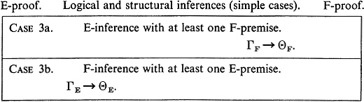
To combine the cases for the 10 propositional rules and 4 structural rules, when we can’t just bypass the inference as above, we write the conclusion as Π_l Γ → Θ, Π₂ where one of Π_l Π₂ is the principal formula (or the C) and the other is empty. We write the premises similarly, where each of Σ₁, Σ₂ or Σ₁, Σ₂, Σ₃, Σ₄ is zero, one or two side formulas (or zero or two C’s). For the rule , then Π_l Π₂, Σ₁, Σ₂, Σ₃, Σ₄ are respectively, where φ is the empty list. The result(s) of our previous treatment of the premise(s) are shown at the tops in each of the next figures (top p. 354), and the result of treating the conclusion at the bottom. As the figures show, we can get from the former to the latter by zero, one or two inferences in G4a. CASES 4b, 5b, 6b, 7b are symmetric (or "dual") to Cases 4a, 5a, 6a, 7a (as 3b, 8b are to 3a, 8a). In each of these cases with an EF-premise (and the inference propositional), (1) and (2) of Case (EF) in the theorem hold for the J in the conclusion in consequence of their holding in the premise(s).

An → ∀-inference is treated under the appropriate one of Cases 3a-5b. By the restriction on variables, b does not occur free in the Γ, Θ. So if the inference is an E-inference, b does not occur free in Γ_F → Θ_F (the

F-part of the premise Δ₁→∧₁); if an F-inference, not in Γ_E→Θ_E. Hence with an EF-premise (Cases 5a, 5b), because (1) in Case (EF) of the theorem is satisfied for the premise, J does not contain b free. Hence the new →∀ satisfies the restriction on variables, and (1) is satisfied for the conclusion.²⁸⁶

Now we treat ∀→. Except in the circumstances described next, this can be handled under one of Cases 3a-5b, with the obvious modification of Cases 4a-5b that the π₁ π₂ (actually, Π₂ is empty now) appear in the premise also (Cases 4a′-5b′). Suppose the premise is an EF-premise, and the A(x) contains the x free. In the predicate calculus without functions, the r must be simply a variable. Say the inference is an E-inference, and that this variable r occurs free in Γ_F →Θ _F but not in ∀xA(x), Γ_E→Θ_E. Then, under (1) for Case (EF) the J for the conclusion is not allowed to contain r free, but the J for the premise may. Supposing it does (Case 9a), let us write it “J(r)” and let y be a variable (maybe x) free for r in J(r) and not occurring free in J(r) (unless y is r).

∀→ with r a variable free in

the J for the premise but not in both

E-proof. the E-part and the F-part of the conclusion. F-proof.

In Case 9a, because r does not occur free in ∀xA(x), Γ _E →Θ _E, the →∀ is legitimate. Similarly, in Case 9b (with r free in A(r) and Γ_E →Θ_E and J(r) but not in ∀xA(x), Γ_F →Θ_F) the ∃→ is legitimate. In the predicate calculus with functions (including individuals), more generally the r may contain free variables c_l. .., c_m and individual symbols e_m+1,.. ., e_n which are parameters of the J for the premise, but are not common to the E-part and the F-part of the conclusion (Cases 9a′, 9b′). Write r also as “r(c₁,. . ., c_m, e_m+1,..., e_n)”, and the J for the premise as “J(c₁,..., c_m, e_m+1,..., e_n)” For Case 9a′ (∀xA(x), Γ_E → Θ_E not containing as parameters c₁. .., c_m, e_m+1,..., e_n), in the E-proof as constructed down through the premise of the inference in question, we can change e_m+1,. .., e_n throughout to respective distinct variables c_m+1,...,c_n not previously occurring in that proof, to obtain instead a proof of A(r(C₁, ..., c_n)), ∀xA(x), Γ_E Θ_E, J(c_l .. ., c_n). Now, instead of inferring ∀yJ(y) as principal formula from J(r) as side formula by one inference in each proof (Case 9a), we can infer ∀y₁. .. ∀y_nJ(y₁,. . ., y_n) from J(c₁,..., c_n) in the E-proof and from J(C₁,..., c_m, e_m+1,..., e_n) in the F-proof by n inferences of the same respective kind.

The rules ∃→ and → ∃ are treated similarly, partly under earlier cases, and partly as new Cases 10a, 10b, 10a′, 10b′.

Summarizing, we repair the E-part or the F-part or both to obtain an E-proof or an F-proof or both, by proceeding downward through the given proof step by step, applying the appropriate case at each step. This leads effectively to one of the three results described in Cases (EF), (E) and (F) of the theorem, determined by the given proof and the given analysis of it. This procedure may involve some unnecessary work in repairing the upper parts of branches that will later be discarded in treating two-premise inferences under Cases 3a, 3b. If we first classify the axioms as EF-, E- and F-, and the two-premise inferences as E- and F-, we can look ahead and anticipate which branches will be discarded.

EXAMPLE 11. First, we show a given proof of E → F in G4a, with the E-part in lightface, the F-part in boldface. To each numbered sequent Δ →∧ in this proof, the like-numbered sequents in the E-proof and the F-proof (below it) are the ones reached by repairing the E-part and the F-part as far as the corresponding sequents Δ_E → Δ_E and Δ_F → Δ_F.287

The E-proof, with formulas replacing the F-part in boldface.

The F-proof, with formulas replacing the E-part in light face.

THEOREM 41.288 (Craig’s interpolation theorem 1957, 1957a.Suppose that in the predicate calculus without equality Then:

(a)If E and F contain a common predicate parameter, then there is a formula I such that and , and the individual and predicate parameters of I are common to E and F.

(b)(Kleene 1952.) If E and F contain no common predicate parameter (or for E ⊃ F without , even if no predicate parameter occurs positively in both or negatively in both),²⁷⁰ then either or .

(c) (Lyndon 1959.)²⁷⁰ For E ⊃ F without , if neither nor , then there is a formula I (without ) such that and , and the individual parameters of I are common to E and F, and a predicate parameter occurs . in I only if it occurs in both E and F.

PROOFS. We may suppose that E⊃F contains no variable both free and bound.²⁵⁹ Assume the hypothesis that . Then by Gentzen’s theorem, , whence (by one →⊃-step upward) . We apply Theorem 40 to a given proof of E → F with the endsequent E → F as the Δ → ∧.

(a) Now assume that E and F have a common predicate parameter. If Case (EF) of Theorem 40 holds, then and where I is the J for the bottom sequent as the Δ ∧. By (1), I contains only individual parameters that are common to E and F. By (2), the predicate parameter of each atomic part of I is in each of E and F, by descent from the C of an axiom. If Case (E) or Case (F) holds instead, we begin by picking a predicate parameter K which is common to E and F, which we can do by hypothesis. Let D be ∀xK(x,. . ., x) (or simply K if K takes 0 arguments). The following table indicates how in these cases we get and , in G4b now.

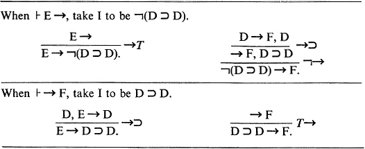
Again, I has only allowed parameters. Now in any case, using →∧ and Gentzen’s theorem (or Theorem 36 Corollary (a)), and .

(b) Suppose, for E ⊃ F without that no predicate parameter occurs positively in both E and F or negatively in both. We shall infer that there is no EF-axiom. It will follow that Case (EF) of Theorem 40 cannot apply; and Cases (E) and (F) lead respectively to and . So assume, for reductio ad absurdum, that there is an EF-axiom C, Γ→Θ , C in the given proof of E→F. Using Lemma 13 § 54, say that the Negative (antecedent) C in this axiom descends into an image in the E of E → F, and the Positive C into one in the F. Then by Lemma 14 the images are Negative and Positive, respectively; so as parts of E and F separately, they are both positive, giving rise to positive occurrences of the predicate parameter of C in both E and F. Similarly, if the Positive C descends into E and the Negative into F, we get negative occurrences of the parameter in both E and F.

(c) Suppose E⊃F does not contain , and that neither nor . Then by Gentzen’s theorem (and one use of →¬), neither nor . So it has to be Case (EF) of Theorem 40 which applies. Consider any predicate parameter occurrence in I; say C_I is the atomic part which contains it. Say C_I is positive as a part of I, and hence Positive as a part of E → I and Negative as a part of I → F. Applying (2) of Case (EF) with Lemma 14, in the proof of E → I the part C_I descends from the second (Positive) C of an axiom C, Γ_E →Θ_E, C, the first (Negative) C of which descends into an image C_E in the E of E → I. This image is Negative as a part of E → I but positive as a part of E. Similarly from the proof of I → F we are led to an image C_F of C which is positive as a part of F. Thus the parameter (assumed to occur positively in I) occurs positively in both E and F. Similarly, a predicate parameter occurring negatively in I occurs negatively in both E and F. —

In the predicate calculus with equality (with or without functions), the statement of Craig’s interpolation theorem can be simplified, since the symbol = (which does not count there as a parameter) is available for building formulas.

THEOREM 42. (Craig’s interpolation theorem with equality 1957a.) In the predicate calculus with equality, if , then there is a formula I such that and and the parameters of I are common to E and F.

PROOF. The method of the proof of Theorem 41 via Theorem 40 does not lend itself directly to excluding from I function parameters (with > 0 places) not common to E and F. However with equality available, we can first use the idea which we met in § 38 of paraphrasing statements employing functions to employ predicates instead.

Suppose that in the predicate calculus with equality. Let A_l . . ., A_m be the open equality axioms for = and the other predicate and function symbols of E⊃F. By Theorem 31 § 29, then in the system consisting of the predicate calculus H with only these predicate and function symbols and with A_l. . ., A_m as additional axioms. Say the (individual and) function symbols in E ⊃ F are f_k,..., f₁ (k ≥ 0). Call the system just described S_k. As illustrated in § 45 ((β), we can replace f_k, . . . , f₁ as symbols for functions (whatever functions the symbols express in a given model) successively by F_k. .., F_x as symbols for the representing predicates of those functions. Thereby, we are led to a system S₀ in which the result E′ D F′ of paraphrasing E ⊃ F to use the representing-predicate symbols in place of the function symbols is provable. The formula E′ contains the same free variables as E, no (individual and) function symbols, and (as predicate parameters) exactly the predicate parameters of E and the representing-predicate symbols replacing (individual and) function symbols of E. The parameters of F′ are similarly related to those of F. The nonlogical axioms B_l.. ., B_l of S₀ are the open equality axioms for = and for the predicate symbols of E′ ⊃ F′, and the formulas ∃!wF_ix₁,..., x_ni, w) for each of the representing-predicate symbols F_l. .., F_fc. Thus each of B_l..., B_l contains at most one predicate parameter, and that parameter occurs in E′ D F′. Suppose the list B₁. . ., B₁ chosen so that in the first part of it B₁.. ., B_k (possibly empty) only predicate parameters in E′ occur, and in the second part B_k+l. . . , B_l (possibly empty) only ones in F′. (Predicate parameters in both E′ and F′ can occur in either part.) Since in S₀, by ∀-eliminations ∀B₁, . . . , ∀B_l in the predicate calculus H. Thence by the deduction theorem etc.,

Now we reason as for Theorem 41 (a), using the Gentzen-type system G4a with only the symbols of S₀ (and therefore no function symbols).²⁶⁵ If Case (E) or (F) of Theorem 40 applies, we employ x=x in the role of the K(x,..., x) there. We obtain thus a formula I′ such that in H

and I′ contains only individual and predicate parameters common to ∀B₁ & ... ∀B_k & E′ and ∀B_k+1 &...&∀Bi⊃F′, and no function parameters. These common parameters are free variables, which clearly must be common to E′ and F′, and predicate parameters, also common to E′ and F′ by the way we split the list B_l..., B_l.

Now ∀B₁,..., ∀B_k and ∀B_k+1,..., ∀Bl, in H. So both E′ ⊃ I′ and I′ ⊃ F′ are deducible in H from ∀B_l. .., ∀B_l, and hence are provable in S₀. By unparaphrasing, we obtain a formula I such that E⊃I and I⊃F are both provable in S_k, and hence in the predicate calculus with equality. That we can thus get back to the original A_l.. ., A_m, E and F is given by the theorem on paraphrasing.289 The free variables of I are the same as of I′ and hence are common to E′, F′, E, F; and the other parameters of I are those predicate parameters of I′ which are common predicate parameters of E′, F′, E, F, and the (individual and) function symbols of E and F which in the passage from S_k to S₀ were replaced by representing-predicate symbols common to E′, F′ Thus all the parameters of I are common to E and F.

Exercises. 56.1. Treat in the manner of Example 11:

(a) The proof in G4 in Example 7 § 54.

(b) The proof of (P(b) ⊃ S) P(b)& → ∀xQ(x) ⊃R ∨ Q(b) obtained by using in order from the bottom up &→, →⊃, ⊃→ and (in one branch) ∀→, →∀.

56.2. Show that in the predicate calculus (for E not containing ): If , then some predicate parameter occurs in F both positively and negatively.

§ 57. Beth’s theorem on definability, Robinson’s consistency theorem. The fifth postulate of Euclid is independent of the other postulates, i.e. it cannot be deduced by logic from them. This was demonstrated, after more than two millenia of speculation, by giving an interpretation which makes the other postulates all true and the fifth postulate false. The Cayley-Kline model for non-Euclidean geometry 1871 (and for the geometry of a bounded part of the plane, Beltrami’s model 1868) is such an interpretation (§ 36). Since then, this has become the standard method in formal axiomatics of showing the independence of one of a list of axioms from the others, or more generally of a given statement from a given list of axioms.

To put this method in our terms, take the case of an axiomatic theory formalizable in the (first-order) predicate calculus without or with equality, say with axioms. Say the axioms are expressed by formulas A₀, A_l A₂,.. . (with their free variables if any having the generality interpretation) and the statement to be proved independent of them by F. Let E₀, E₁, E₂,... be the closures of A₀, A₁ A₂,.... The traditional method then simply applies the consistency theorem (cf. end § 52),

with informal use of *12a (contraposition), *82b and *55c (§§ 3, 25).

Similarly, the completeness theorem,

when contraposed, says that in principle the traditional method must always work; i.e., whenever the statement in question does not follow by logic from the axioms, it has to be false under an interpretation which makes all the axioms true (cf. § 53).

Just as we usually wish to have the axioms of a formal theory independent, we would also like to have the primitive concepts independent, i.e. such that no one of them can be defined from the others. How can it be shown that, in the theory based on certain axioms A₀, A_l, A₂,.. ., a certain concept q cannot be defined from the other concepts p₀, p_l p₂,... of the theory. Padoa 1900 used a counterpart of the more familiar method of showing axioms to be independent. Namely, he gave two interpretations (with the same domain) such that the axioms A₀, A_l A₂, .. . are all true under both, p₀, p₁ p₂,. .. have the same values under both, but q has different values under the two. For, if there were a definition of q from p₀,p₁,p₂,... in the theory with A₀, A_l A₂,. .. as the axioms, that definition should determine the value of q from the values of p₀, p_l p₂,. . . for any values of the latter which are compatible with A₀, A₁, A₂,.. . all being true. Thus it should not be possible to make q have different values when P₀, P₁, P₂..., have the same values and A₀, A_l A₂, ... are all true.

We now study this method in modern terms. We generalize it to discuss the definability of q from p₀, p_l p₂,. . . when the closures E₀, E_l E₂,. . . of the axioms A₀, A₁ A₂,. . . may obtain still other parameters r₀, r₁, r₂,... Our notation is for the most general case, of axioms and parameters in each of the two lists. The reader can supply the modifications when one or more of these lists are finite or even empty. We take q and all the listed parameters to be distinct. For the present, each parameter in the two lists (which together with q must include all occurring in the closed axioms E₀, E₁, E₂,. ..) shall be a (proposition or) predicate symbol or an individual symbol, q shall be an n-place predicate symbol Q (with n ≥ 0), and the logic shall be the predicate calculus without equality.

Padoa’s method is equivalent (by contraposition etc.) to the implication: {Q is definable from p₀, p₁ p₂,. . . in the theory based on E₀, E₁ E₂,. . . as axioms} -→ {each two interpretations of the parameters Q, p₀, p_l p₂,. .., r₀ r₁ r₂.... which make E₀, E_l E₂,. .. all true and give p₀, p_l p₂,.. . the same values give Q the same value}, or briefly Dfb_E → Dfd_I.

First we analyze Dfb_E. We take it to mean that a suitable defining expression can be given for Q(x_l. . ., x_n) (as definiendum). Such an expression shall be in the language of the theory, i.e. the predicate calculus with the named parameters. It shall contain as free variables only x₁. . ., x_n, and as other parameters only ones from the list p₀, p_l p₂,..., of which it can contain only finitely many, say only p₀,. . . , p_s. Say the defining expression or definiens is R(x_l . . ., x_n, p₀,. . ., p_s). While the logic is the predicate calculus, we must have s ≥ 0 with at least one predicate parameter among p₀,. . ., p_s, as a definiens cannot be constructed without using a predicate parameter. Finally, we must express that R(x₁. . ., x_n, p₀,. . ., p_s) is a definiens for Q(x₁, . . ., x_n) in the theory based on E₀, E_l E₂,.. .. This means that, for each domain D and assignment which satisfy all of E₀, Ex, E₂,. . ., the formula R(x₁,. . ., x_n, p₀,. . ., p_s) shall have the same truth value as Q(x_l. . ., x_n ), for all values in D of x₁ .. ., x_n. Thus we are led to the following rendering of Dfb_E.290

For some formula R(x_l . .., x_n, p₀,.. ., p_s) containing only the parameters shown,

We say in this case that (model-theoretically) Q is definable explicitly from p₀, p_l p₂,. . . in the theory based on E₀, E_l E₂,. . . as the closed axioms, or that E₀, E₁ E₂, . . . make Q so definable. Further, for such an R(x_l.. . , x_n, p₀,. . ., p_s), we say that {model-theoretically) E₀, E_l E₂,. . . define Q explicitly from p₀, . . . , p_s as R(x_l. . ., x_n, p₀,.. ., p_s).

We can replace “E₀, E₁ E₂,.. . =" equivalently by “for some d, E₀,.. ., E_d ” [by the completeness and consistency of the predicate calculus], and further by “for some d, E₀ &. . . & E_d ⊃” [by ⊃-introd. etc.]. Only finitely many parameters can occur in E₀ & . . . & E_d we can increase the s in R(X₁,. . . , x_n, p₀, . . . , p_s) if necessary so only p₀,. . ., p_s, r₀,. . ., r_t, occur in E₀ & . . . & E_d. By these steps, is equivalent to the following.

: For some finite conjunction E(Q, p₀,. . ., p_s, r₀,. . ., r_t) of

E₀, E_l E₂,. . . and some formula R(x₁, . . . , x_n, p₀,. . ., p_s), each containing only the parameters shown,

We say in this case that (proof-theoretically) Q is definable explicitly from in the theory based onorQ so definable. Further, (proof theoretically) Q explicitly from p₀,. . ., p_s as R(x_l. . ., x_n, p₀,. . . , p_s). The lower version here can be used with any formula E(Q, p₀,. . ., p_s, r₀,. . ., r_t,) with only the parameters shown, whether or not it is a finite conjunction of E₀, E₁ E₂,.. ..291

Next we analyze Dfd_I. Let Q′, r′₀, r′, r′₂,... be new parameters of the same respective kinds (predicate or individual) and numbers of argument places as Q, r₀, r_l r₂,. . . ; and let E′₀, E′₁, E′₂,. . . come from E₀, E_l E₂,. . . by substituting Q′, r′₁, r′₂, . . . for Q, r₀, r_l, r₂,. . ., respectively. Instead of having two interpretations of Q, p₀, p₁ p₂,. . ., r₀, r_l, r₂,. . . which make E₀, E_l E₂,. . . all true and give p₀, p_l p₂,. .. the same values, it is equivalent to have one interpretation of Q, Q′, p₀, p_l p₂,..., r₀, r′₀, r₁ r′₁, r₂, r′₂,. . . which make E₀, E′₀, E₁ E′₁, E₂, E′₂,. .. all true. This device leads to the following rendering of Dfd_I.

We say in this case that (model-theoretically) Q is defined implicitly from p₀, p₁, p₂, . . . (with r₀, r₁ r₂, . . . as auxiliary parameters) by, or in the theory based on, E₀, E₁ E₂,. . ..

By the same transformations as we used on , this condition is equivalent to the following, where E(Q′, p₀, . . ., p_s, r₀′, . . . , r′_t) is the result of substituting Q′, r₀, . . ., r′_t for Q, r₀,. . . , r_t in E(Q, p₀, . . . , p_s, r₀,. . . , r_t).

: For some finite conjunction E(Q, p₀,. . ., p_s, r₀,. . ., r_t) of E₀, E₁, E₂,. . . containing only the parameters shown,

We say in this case that (proof-theoretically) Q is defined implicitly from (with as axuiliary parameters) by, or in the theory based on,

Summarizing, Padoa’s method rests on an implication which (after contraposition) we have rendered in model theory by , or equivalently (using and ) in proof theory by .

It is a simple exercise to corroborate Padoa’s method proof-theoretically by establishing . In fact, any formula E(Q, p₀,. . ., p_s, r₀,. . ., r_t) which makes Q definable explicitly from p₀,..., p_s also defines Q implicitly from p₀,.. ., p_s (Exercise 57.1).

Our analysis thus far has been a straightforward application of results which have been available since 1930 (consistency with respect to validity e.g. Hilbert and Ackermann 1928 bottom p. 73, the deduction theorem 1930, Gödel’s completeness theorem 1930).

Now we inquire whether Padoa’s method is complete. That is, will it always work, whenever one primitive concept in an axiomatic theory is in fact independent of the others? An affirmative answer would be equivalent via contraposition to saying that, whenever it is impossible to satisfy the closed axioms E₀, E₁ E₂,. . . by two values of Q compatibly with given values of p₀, p₁ p₂,.. ., the resulting implicit model-theoretic dependence of Q on p₀, p₁, p₂,. . . must be expressible by an explicit definition within the syntactical limitations of the language. This is certainly not obvious.

However, the completeness of Padoa’s method was established with a trivial exception by Beth in 1953.292 The exception is when p₀,. .., p_s include no predicate parameter; without a predicate parameter, we can’t build a definiens R(x₁,. .., x_n, p₀,. . ., p_s) in the predicate calculus without equality. The provision for auxiliary parameters r₀,. . ., r_t in the implicit definition not appearing in the definiens, and some other generalizations of Beth’s result, were given by Craig in 1957a.

By the foregoing preliminary analysis, what we need is , or equivalently . For the latter, it will suffice to show that any formula E(Q, p₀,. -p., p_s, r₀,. . ., r,) which (proof-theoretically) defines Q implicitly from p₀,. . ., p_s also makes Q definable explicitly from p₀,. . ., p_s, as we state in:

THEOREM 43. (Beth’s theorem on definability 1953.) Let the symbolism and logic be those of the predicate calculus without equality but allowing individuals. Let the notation be as explained above (in particular, each formula shall contain only the distinct parameters shown). Suppose that

i.e. E(Q, p₀,. . ., p_s, r₀,. . ., r_t) defines Q implicitly from p₀,. . ., p_s with r₀,. . ., r_t as auxiliary parameters. Then:

(a) If one of p₀,. . ., p_s is a predicate parameter, there is a formula R(x₁. . ., x_n, p₀, . . ., p_s) such that

,

i.e. E(Q, p₀,. . ., p_s, r₀,. . ., r_t) makes Q definable explicitly from p₀,..., p_s.

(b) If none of p₀, . . . , p_s is a predicate parameter occurring in E(Q, p₀, . . . , p_s, r₀, . . . , r_t)then

,

i.e. E(Q, p₀, . . ., p_s, r₀,. . ., r_t) defines Q either as the constant predicate “truth” or as the constant predicate “falsity”.

Proof. Using the main hypothesis with the propositional calculus,

This we take as the “” for Craig’s interpolation theorem (Theorem 41).

(a_x) Suppose one of p₀,..., p_s is a predicate parameter occurring in E(Q, p₀,. . ., p_s, r₀,. .., r_t). Then by (a) of Theorem 41, there is a formula I such that and I contains only parameters common to E and F. But at most x_l. .., x_n, p₀,.. ., p_s are common to E and F. So letting R(x₁,. .., x_n, p₀,. . ., p_s) be this I, the structural requirement is met, and

The proof of the formula in (iii) remains a proof on substituting in it Q, r₀,. . . , r_t for Q′, r′₀,. . ., r′_t.⁸⁶ So

From (ii) and (iv) by propositional calculus,

(a₂) If one of p₀,. . ., p_s is a predicate parameter, but no predicate parameter among p₀, . .., p_s occurs in E(Q, p₀,.. ., p_s, r₀,..., r_t), then (b) (to be established next) applies, after which we can trivially construct an R(x_x,. . ., x_n, p₀,.. ., p_s).

(b) Suppose no predicate parameter among p₀,.. ., p_s occurs in E(Q, p₀, p_s, r₀,. .., r_t). Then by Theorem 41 (b),

Using propositional calculus (*60, *49; or IM *58b) on (vi-1), and substituting into (vi-2),

Now we take the case of the predicate calculus with equality and functions. The parameter q for Padoa’s method can now be either an n-place predicate symbol Q or an tf-place function symbol g (with n ≥ 0).

THEOREM 44. (Beth’s theorem on definability, in the predicate calculus with equality and functions.) In the predicate calculus with equality and functions, and with the notation as explained:

(A) If

then there is a formula R(x₁,..., x_n, p₀,. .., p_s) such that

(B) If

then there is a formula R(x₁,. . ., x_n, p₀,. .., p_s) such that

then there is a formula R(x₁,. . ., x_n, p₀,. .., p_s) such that

Proof, (a) As before, except using Theorem 42, which gives us an R(x₁,. .., x_n, p₀,. . ., p_s) in all cases.

(b) In the predicate calculus with equality, g(x₁. .., x_n-1)=g′(x₁,..., x_n-1) is equivalent to g(x₁,. .., x_n-1) = x_n ∼ g′(x₁,.. ., x_n-1)=x_n. Now the above reasoning applies with g(x₁. . ., x_n-1) = x_n in place of Q(x₁,. . ., x_n). —

As we remarked in § 38,¹⁵⁷ in N with the symbol . and its axioms 20 and 21 omitted, the representing predicate a ^. b=c of a ^. b cannot be expressed. Hence by Theorem 44(B) (contraposed),²⁵¹ Padoa’s method applies; i.e. there are two models of N, with the same domain D and the same assignment to 0, ′, + (with = meaning equality), in which ^. has different functions as values. —

As a second application of Craig’s interpolation theorem, we establish the consistency theorem of A. Robinson 1956, 1963 p. 114. Robinson proved this independently of Craig’s theorem, and used it to prove the theorem of Beth.

The problem is this. Suppose we have two consistent formal systems S₁ and S₂, with axioms A₀, A₁ A₂,. . . and B₀, B_l B₂,. . . and nonvariable parameters p₀, p_l, p₂,.. . and q₀, q_l, q₂,. .., respectively. (The reader may substitute finite lists.) Will we obtain a consistent system S₁ ∪ S₂ by combining S₁ and S₂ so the axioms of S₁∪S₂ are A₀, B₀, A₁, B₁ A₂, B₂,... and the nonvariable parameters are p₀, q₀, p₁, q₁, p₂, q₂,... (each list with repetitions allowed)?

Not necessarily. For, let S₁ be number theory N with the addition of GödePs formula (which is true in the standard model, but unprovable in N), and S₂ be N with C_p added. The systems S₁ and S₂ are each consistent, using the consistency of N (cf. § 47, where S₂ is called "M"). But the union S₁ ∪S₂ is not. Clearly the difficulty here is that the common portion N of S₁ and S₂ is incomplete, so that in S₁ and in S₂ we could extend N in two different ways, each consistent with N, but inconsistent with each other.

This example suggests an additional hypothesis under which we can hope to answer the question affirmatively: the two formal systems should be in “complete agreement” on topics of mutual concern; i.e., for each closed formula I which contains only parameters common to S₁ and S₂, the same one of the two formulas I and I should be provable in each of S₁ and S₂.

The reasoning here, as in Gödel’s completeness theorem and most other passages in this chapter dealing with formulas, does not depend on the formulas being given effectively, as the axioms of a formal system are required to be (cf. §§ 37, 43). So in stating the theorem, we allow S₁ and S₂ alternatively to be sets of formulas based on the predicate calculus, analogously to (the set of provable formulas of) a formal system based on the predicate calculus, but without the effectiveness requirement for the axioms.

THEOREM 45. (Robinson’s consistency theorem, 1956.) Let S₁ and S₂ be formal systems (or sets of formulas) based on the predicate calculus without or with functions and equality. Suppose that S₁ and S₂ are each simply consistent. Suppose they are in complete agreement, i.e. for each closed formula I in the common portion (or intersection) of their symbolisms, one of I and nl is provable in both S₁ and S₂. Then the combined system (or union) S₁∪S₂ is simply consistent.

Proof. We begin with the case of the predicate calculus without functions and equality but admitting individuals. Let E₀, E₁, E₂,. .. and F₀, F₁, F₂,. . . be the closures of the axioms of S₁ and S₂, respectively. Suppose S₁∪S₂ is not consistent, so a contradiction K & K is deducible from E₀, F₀, E₁, F₁, E₂, F₂,., . in the predicate calculus. Let E₀,..., E_c, F₀,. .., F_d be those of E₀, F₀, E₁, F₁, E₂, F₂,.. . which are used in a given deduction of K & K. Thus E₀,.. ., E_c, F₀,..., F_d h K & K in the predicate calculus. Thence by propositional calculus,

We take this as the “” for Theorem 41. If no predicate parameter is common to E₀ & ... & E_c and -j(F₀ & ... & F_d), then by Theorem 41 (b) h i(E₀ & ... & E_c) or h -i(F₀ & ... & F_d). But then S₁ or S₂, respectively, is inconsistent, contrary to hypothesis. If some predicate parameter is common, then by Theorem 41 (a) there is a formula I such that

and I contains only parameters common to E₀ & ... & E_c and (F₀ &... & F_d). So I is closed, since E₀, E₁, E₂,.. . and F₀, F₁, F₂,... are closed. By the hypothesis of complete agreement, in the predicate calculus

But in the first case, (ii) and (iv-1) are incompatible with the consistency of S₂; for, contraposing (ii) (*13 in § 24), . In the second case, (i) and (iii-2) are incompatible with the consistency of S_1#

For the predicate calculus with functions and equality, we use Theorem 42 instead.

EXERCISE 57.1. Show that, if E(Q₀, p₀,..., p_s, r₀,..., r_t) defines Q explicitly from p₀,. . ., p_s, it does so implicitly.

---

219 Many of the results of this chapter belong to classical nonfinitary model theory, and thus not to metamathematics (§37).

²²⁰ Although characteristic features of the predicate calculus go back to Frege 1879, the first explicit formulation of it as a separate formal system is perhaps in Hilbert and Ackermann 1928, according to Church 1956 pp. 288 ff.

²²¹ Thus in § 2 (1) the parameters are P, Q, R; in § 17 Example 1 they are P(x), Q, y or P(—), Q, y or simply P, Q, y; in § 28 Example 1, f, x for the term P and f for the formula; and in § 29 Example 2, P, f (but not =). (However in this chapter until § 52, we shall not use § 29, which gives a fixed preassigned value to =.)

²²² If F is a formula of the propositional calculus simply, we don’t need to mention any domain D, and a falsifying assignment or counterexample can be simply an assignment of t’s and f’s to the atoms of F which makes F f.

²²³ In some respects it more resembles Kanger 1957, as the author learned after working it out.

Some of the other proofs of Godel’s completeness theorem are in Hilbert and Acker-mann 1938 (= 2nd ed. of 1928), Hilbert and Bernays 1939, Mostowski 1948b, Henkin 1949, 1963, Rasiowa and Sikorski 1950, Rieger 1951, A. Robinson 1951, 1963, Beth 1951, Kleene IM (1952b), 1958. Those listed in bold face apply topology or algebra.

²²⁴ An alternative representation of our search is obtained by simply omitting the verbal explanations given above, but writing the nine numbered formulas in two columns, marked true (t) and false (f). After (6), where we have a choice, the columns split into respective left and right subcolumns (i) and (ii). This gives what Beth 1955, 1959 calls a semantic tableau:

more efficient than the sequent trees, since they do not require us to recopy formulas whose status is not being changed. But they do not show the individual situations as simply (e.g. that when (8) has just been introduced, Δ is (4), (8) and A is (5)). Hence we prefer to use the sequent trees in the proof of Gödel’s completeness theorem and other theoretical uses.²⁶⁸ (The tableau here does show explicitly that, when (8) has just been introduced, it suffices to make (2), (4), (6), (8) t and (1), (3), (5) f. This kind of information taken with the structure of such lists, is enough for recognizing the counterexamples. But, altogether, we believe what we shall be doing is more easily visualized in terms of the sequent trees.)

²²⁵ The reasoning in this paragraph is to make our procedure in § 49 understandable in advance. The fact that by it we do succeed in proving Godel’s completeness theorem would be sufficient justification for it.

²²⁶ We showed such a splitting in § 30 Example 5, where it was a question of finding an example for a formula E rather than a counterexample. Until § 52, our evaluation rules are those of the predicate calculus § 17 or the predicate calculus with functions § 28, not those of the predicate calculus with equality § 29. Meanwhile, if = should occur in any of our formulas it is to be treated like any other predicate parameter.

²²⁷ Also, we can easily adapt the proof of Theorem VII to show directly (without using GödeFs completeness theorem) that there is no algorithm for validity.

²²⁸ The logical functions or predicates can always be of degree ^ 1 § 46, by IM Theorems 38 and 40 pp. 398, 401 with Theorem XI (Post’s theorem) IM p. 293. Further information about these predicates is given in Mostowski 1954 pp. 284-285.

²²⁹ There could be doubt only when the A or the A of one of the sequents Δ →; λ contains several occurrences of the same formula, or with the rules ∀→ and →∃ when the Δ of the λ of the sequent below the line contains congruent formulas ∀xA(x) and ∀yA(y), or ∃xA(x) and ∃yA(y).

²³⁰ We use E’s and F’s to allow "A₁,..., A_m →B₁,. .., B_n" to denote various sequents in a tree having the fixed sequent E_l. . ., E_k→F₁ . .., F_l at the bottom.

²³¹ The reader who is willing to agree that a search plan can be formulated (in this Case (A)) which makes Lemma 8 true may skip the details by passing to Lemma 9.

²³² The exclusion of variables occurring free in E₁ ..., E_k → F₁ ..., F_i from also occurring bound is necessary. Cf. Exercise 49.2.

²³³ For a sequent E₁,..., E₂ →F₁,..., F_i containing no variables free or bound, and no individual symbols, i.e. a sequent of the propositional calculus simply, we can alternatively forget about the list u₀,..., U_p, a₀, a₁ a₂,.. ..²²² The following discussion, omitting what is then irrelevant, gives a new treatment of the completeness problem for the propositional calculus.

²³⁴ Actually (in this Case (A)), for an infinite path it is easily seen that N₀ terms t₀, t₁, t₂,... must be activated, or we would run out of steps to perform at a finite stage. (This remark isn’t necessary for our purposes, and it won’t always be so in Case (B) § 50.)

²³⁵ In our search plan, when u₀,..., u_p is empty, we activate a₀ by fiat at the beginning to be sure of having it. But it is more economical to wait then for a₀ to be activated by the first →∀ or ∃→ when one of these can be reached before we need to perform an ∀→ or →∃ ; along any unclosed path in which we can’t do this, a₀ should be activated by fiat (before termination). Steps may be performed in any convenient order for a while, provided that a routine like the one in our plan is instituted eventually along each infinite path. In applying →∀ or ∃→ to a sequent in which one of the previously activated variables does not occur, that variable may be used as the b instead of a newly activated variable. In applying ∀→ or →∃ when the A(x) does not contain the x free, it is sufficient to use only one r. Also cf. the "first approach" in Example 3 § 48.

²³⁶ For a terminated unclosed branch, it is sufficient (by the rationale of our searches, or specifically by Lemma 6 (b)) to make just the formulas in the top sequent have the right values (as illustrated in Example 1). However, often the best way to see that we can do this is by the reasoning we give here.

²³⁷In other forms this is in Brouwer 1924, and implicitly in Brouwer 1923a and Skolem1922-3 p. 222 Cf. Kleene and Vesley 1965 p. 59.

²³⁸ Using a different mechanical verification process than the present one, this basic discovery is quite clearly contained in Skolem 1922-3 pp. 220-222 (which was not known to Godel in 1930). Cf. Footnote 252 below.

²³⁹ Gentzen-type systems G1, G2, G3, G3a are discussed in IM §§ 77-80, which we shall cite more specifically in § 54. The present system G4 is very close to (73, to the system L of Beth 1959 p. 282, and to LC in Kanger 1957. The first 8 rules coincide with the propositional rules of Ketonen 1944.

²⁴⁰ G3 has the feature, but not Gl, G2, G3a.

²⁴¹ Cf. IM pp. 106-107. In IM “branch” is used where we have been saying “path”, with both Hilbert-type and Gentzen-type systems. (Contrary to botany, a “branch” starts from, or reaches to, the bottom, not just from the lowest “branching”.) The term in Hilbert and Bernays 1934 is “proof thread (Beweisfaden)”.

²⁴² One of the interesting cases is that ..., E₂, E₁, E₀ are the closures of the axioms of a formal system like N of § 38, and instead of F₀, F₁, F₂,... we have a single formula F. We shall review this application at the end of § 52. However, it is not required for the present treatment that the formulas ..., E₂, E₁, E₀ (or F₀, F₁, F₂,...) be given effectively, as the axioms of a formal system should be (cf. §§ 37, 43). (For the result mentioned in Footnote 228 with infinitely many formulas, the lists must be effective, so that E_i and F_i can be found effectively from i.)

²⁴³ In this book we do not attempt to consider languages for the predicate calculus with uncountably many symbols, and hence uncountably many formulas. Such languages are highly non-constructive. However, Malcev 1936, Henkin 1950, A. Robinson 1951, etc. have studied them, and found model-theoretic applications. Propositional calculus with uncountably many symbols is allowed in Gödel 1931—2b.

²⁴⁴ The reader who skipped the details of the search plan in Case (A) should observe one new point (after which he can pass to Cases (C) and (D)): If the tree is closed, and thus finite, then only finitely many of..., E₂, E₁, E₀ and F₀, F₁, F₂,... (say at most E_d,..., E₀ and F₀,..., F_d) can have taken into account in constructing it by the 14 rules and recognizing it as closed by the axiom schema (×).

²⁴⁵ The reader who has been skipping the details of the search plan may pass to the remarks on Lemmas 8 and 9.

²⁴⁶ If there are none of (ii), the list a_i u_i, u_i1, u_i2, u_i3,... reduces to a_i (i = 0, 1, 2,...); then there must be χ₀ of the symbols (i), or we would be back in Case (A) or (B). If there are some of (ii) but none of (i), the list u₀, u₁, u₂,... disappears, and a₀ should be activated initially.

²⁴⁷ These versions (except “compactness” in (b)), for Cases (A) and (B), can be established by the reasoning in Skolem 1920 plus the trivial argument (end § 49) that, if we come out with a finite domain, an element can be split into χ₀ elements. More details of the history are in Footnote 252 below.

²⁴⁸ If we interpret “A₁ & ... & A_m” for m = 0 to be (P & P) (or P ⊃ P), and “B₁ V ... V B_n” for n = 0 to be P & P (or (P ⊃ P)), then (b) holds without the restriction to m, n > 0.

²⁴⁹ The proof of Theorem 33 is good under either meaning of . We aren’t defining another formal system G4 for the case of the predicate calculus with equality, as we did with H in § 29.

²⁵⁰ Often one speaks loosely of a mathematical system satisfying some axioms, or of some axioms being true under an interpretation, when it is to be understood that free variables occurring in the axioms have the generality interpretation. The precise meaning is then what we have rendered here in the definition of “model”.

In technical discussions, when we say that formulas are satisfiable, in general or in a given domain, we mean precisely that the formulas themselves are satisfiable (but not necessarily their closures, if the formulas are open); and similarly with “satisfying assignment”, “falsifiable”, “counterexample”, etc.

²⁵¹ In the illustrations by G and N, since the equality axioms for = and their function symbols are all provable, by Corollary Theorem 31 § 29 it makes no essential difference in the proof-theoretic notions whether the logic is the predicate calculus without or with equality (Axioms E1-E3, or Axioms 16, 17, are redundant in the latter case). But (for systems with = as a symbol) the model-theoretic notions of the predicate calculus with equality are usually the ones that primarily interest us.

²⁵² According to modern scholarship (van Heijenoort 1967), there are serious gaps in Löwenheim’s attempted proof 1915 of the theorem which bears his name. What Lowenheim stated is our Theorem 35₌ (a) (except without all our possibilities for the definition of “formula”).

The first correct proof of this proposition is in Skolem 1920, where it is generalized to formulas (giving essentially our Theorem 35₌ (b) without the “compactness” part). In this proof, Skolem used the set-theoretic axiom of choice (§ 35), and his normal form 1920 for formulas of the pure predicate calculus (cf. Hilbert and Bernays 1934 pp. 158 ff., IM p. 435).

The work of establishing the reducibility to Skolem normal form can be spared, however. By using instead any prenex form (Theorem 27 § 25), we get a very simple proof in the following manner (Skolem 1929 p. 24, Kleene 1958 p. 139). Say e.g. a prenex form of E is ∀w∃x∀y∃zA(w, x, y, z) where A(w, x, y, z) is a quantifier-free formula containing just the distinct variables v, w, x, y, z and two function symbols ,λ(—). Using the axiom of choice, then E is satisfied in a non-empty domain D by a certain assignment, if and only if ∀w∀yA(w, β(w), y, δ(w, y)) (where β(—), δ(—, —) are new function symbols) is satisfied in D by that assignment plus some assignment to β, δ. But a domain and satisfying assignment for the latter formula remain such, when the domain is cut down from D to the countable domain D^* consisting of just the values of v and and the other members of D obtainable thence by repeated applications of the functions evaluating λ, β and δ, and the functions and predicates in the assignment are “restricted” to D*.

These axiom-of-choice proofs establish that, given any model of a formula or list of formulas, there is a finite or countably infinite submodel of the given model (in the sense just illustrated). No special attention is required to =, whose meaning of identity, if used in the given model, carries through to the new model.

The device (used in § 48-50) of picking truth values of atoms toward building up a satisfying (or falsifying) assignment, independently of the values the atoms have in a given such assignment, avoids the use of the axiom of choice, but sacrifices the submodel result, and (at least as ordinarily carried out) required a restoration of the usual meaning of = (as in § 52) in the case of the predicate calculus with equality. In 1922-3 pp. 220-222 and 1929 pp. 24-29, Skolem used this device to give proofs of the Löwenheim-Skolem theorem (in versions like our Theorem 35 (a) and (b)) which at least implicitly (but in retrospect quite obviously) establish everything in Gödel’s 1930 completeness theorem (including compactness), with two exceptions. First, only a form of the basic discovery (beginning § 50) is established; it is not shown further that, when validity is confirmed by the finite mechanical process in Skolem’s treatment, one has provability in Hilbert’s sense. Skolem could hardly have done this in 1922-3, since Hilbert’s proof-theoretical formulation of the completeness problem only became clearly defined in Hilbert and Ackermann 1928 p. 68. So we can say that Skolem in 1922-3 discovered the completeness of intuitive logic (of first order), and independently Gödel in 1930 (not knowing Skolem 1922-3 or 1929) discovered the completeness of formal logic. Secondly, Skolem does not give the supplementary argument to restore the meaning of =. (There is no explicit discussion in his 1920, 1922-3 or 1929 of the impact of equality on the theorems in question, and it is not always clear what he intends regarding =.)

According to Dreben and van Heijenoort (in the introductory note to the translation of Skolem 1928 in van Heijenoort 1967), one can get Gödel’s 1930 theorem (without equality) by combining arguments in Skolem 1920 and 1922-3, or 1929, with ones in Herbrand 1930 (plus now-familiar results on prenex form, say our Theorems 27 with 12_Pd and 19).

The treatments of Gödel’s completeness theorem cited above do not deal with functions directly, as is done in Cases (C) and (D) § 50 (exceptions: the argument obtained by combining Skolem and Herbrand, the related treatment in Kleene 1958 and 1961 outlined in Footnote 280 below). Of course, since Hilbert and Bernays 1934, the results could be extended to functions via a replacement of functions by their representing predicates (cf. §§ 38, 45; IM p. 424).

²⁵³ Utilizing this observation, Hilbert and Bernays 1939 pp. 234-253 formalize their proof of Gödel’s completeness theorem in (essentially) the number-theoretic system N, and thus establish the following metamathematical completeness theorem for the pure predicate calculus (cf. IM p. 395).

The addition to the predicate calculus of an unprovable predicate letter formula for use as an axiom schema would cause the number-theoretic formal system based on the predicate calculus and the nonlogical axioms of N (§ 38) to become ω-inconsistent (§ 47).

²⁵⁴ Cf. IM p. 420 Example 13. Axiom Al and the predicate symbol (x) (“x is a class”) can then be omitted.

Skolem’s is not a paradox in the sense of an outright contradiction, but rather a kind of anomaly. For, there is an explanation: the “enumerating set” of ordered pairs, by which D* is put into 1-1 correspondence with the natural numbers, is not itself a set admitted in the axiomatic set theory.

²⁵⁵ Not however with quite the version in Gödel 1931, where the incompleteness is given for “Principia Mathematica [Whitehead and Russell 1910-13] and related systems”. PM is not of the form {(first-order) predicate calculus} + {number-theoretic axiom system}. Number-theoretic systems of that form (like N in § 38) came in with Hilbert 1928, so they are sometimes called Hilbert arithmetic. In 1931-2 (reporting a colloquium held January 22, 1931), Gödel states his incompleteness theorem for such a formal system, with all the usual axioms of elementary number theory.

When the author pointed out the connection between Skolem’s and Gödel’s theorems in IM (1925b) p. 430 and 1956 § 18, he knew of no earlier mention of it in the literature. Recently, he has come across 2 lines in Gödel’s review of Skolem 1933 (1934a p. 194 lines 10–11) and 3 in Henkin 1950 (p. 91 lines 8-10) alluding to such a connection.

²⁵⁶ Still another pair of circumstances shows very simply that there must be non standard models. By the hierarchy theorem of Kleene 1943, the predicates definable in the symbolism of N fall into a hierarchy, with predicates of successively higher levels requiring more and more quantifiers in their definitions (§46 including Exercises 46.8,46.9 (a)). This of course is proved by reasoning with the standard model of number theory. But by IM Theorem 40 pp. 401-402,²²⁸ all the satisfying predicates in Gödel’s completeness theorem are definable using just two quantifiers. These results would be incompatible, if the model for the latter were the standard one. This proof is given in detail in IM pp. 428-429.

²⁵⁷ To any effective list A₀, A_l, A₂, . . . not sufficient to give us the formulas C_a of § 43 using in them only the parameters 0, ′, + , ·, or not including Axs. 14, 15, 18-21, we can first add the axioms of N § 38.

²⁵⁸ 1934. p. 160 Skolem like Peano used the positive integers instead of the natural numbers.

²⁵⁹ To deal with formulas containing variables both free and bound, we can use Theorem 25 as in the proof of Theorem 37.

²⁶⁰ As the chart shows, the gap can be filled by reading the proofs of IM Theorems 46 and 48 §§ 77, 78, and using for our applications the Gentzen-type systems G4a and G4b introduced below. For agreement with IM and Kleene 1952, we can optionally take “A B” in our systems to be an abbreviation for .

²⁶¹ In this chapter, the absence of a "°" on a theorem concerning provability in Gentzen-type systems means that there is a known intuitionistic version of the theorem (sometimes with qualifications), using the intuitionistic version of one of the systems Gl, G2, G3, G3a, G. When we do not indicate otherwise, this intuitionistic version can be found in IM or Kleene 1952.

²⁶² For references to Beth’s intuitionistic model theory or semantics, see Kleene and Vesley 1965 bottom p. 81.

²⁶³ Cf. IM pp. 482-485.

²⁶⁴ However, this approach is used in IM § 80 to show some classically provable formulas of the predicate calculus to be intuitionistically unprovable. The intuitionistic unprovability is shown by identifying an infinite branch in the sequent tree constructed upward using the Gentzen-type system G3. Also cf. Curry 1950.

²⁶⁵ Exception: (individual and) function symbols may be introduced which are not in the endsequent, if they are allowed under the formation rules of the system in question. But, by our completeness argument (§§ 48-50), any provable (and hence valid) sequent can be proved in that system G4 which has only its own (individual,) function and predicate symbols. Or simply in proof theory, in a given proof we can replace the (individual,) function and predicate symbols not present in the endsequent (or in H, in the endformula), as in Theorem 31 § 29 and in the proof-theoretic treatment of sub stitution (Footnote 86 § 25).

²⁶⁶ We are using “direct” here in a more general sense than at the ends of §§ 13, 25. There a proof or method of proof was considered “indirect” when, to prove F, we begin by deducing a contradiction from F (thus proving F, before using -elimination) or use some variant of that device.

In §§13 (early), 21, 23 etc., “direct” has still another sense in “direct rule” vs. “subsidiary deduction rule”.

The directness of a proof in G1 without cut compared to Gl using a cut is illustrated in IM pp. 448-449 Example 1.

²⁶⁷ Herbrand 1930 showed that any provable formula of the predicate calculus can be proved without using modus ponens in the part of the proof employing quantifiers (§ 55). Gentzen reached his “Hauptsatz” or “normal form theorem” by following his own direction of investigation, not using this result of Herbrand. Gentzen 1934-5 is crystal clear, while Herbrand 1930 has only recently been fully elucidated.²⁷⁹

²⁶⁸ But Gentzen’s work, and related work of others, has a practical side. We have seen this in connection with our format (B₂) end § 13. This can be obtained by taking a suitable Gentzen-type sequent system, and using the sequents without each time writing the formulas of the antecedent. Thus Gentzen 1934–5 obtained “natural deduction systems”. Jas´kowski 1934 introduced such systems directly, at the suggestion of Lukasiewicz in seminars in 1926. Beth’s semantic tableaux are closely related.²²⁴ But we have preferred in our practice of logic to operate flexibly using derived rules, rather than to freeze our practice into a particular such system. Cf. § 25, Prawitz 1965.

²⁶⁹ The subformulas of a given formula without as a succedent or antecedent formula are accordingly classifiable as succedent subformulas (Positive) and antecedent subformulas (Negative). Cf. Kleene 1952 pp. 10-11, which the present discussion (including Lemma 14) follows in substance. The terms “ancestor”, “descendant” and “image” are from that paper. “Subformula” should have been defined there as in IM or here (as noted by V. P. Orevkov); this is corrected in the 1967 edition.

²⁷⁰ The method of adapting the discussion to the presence of was indicated in the final paragraph of § 54.

²⁷¹ Our search procedure in §§ 49-50 will lead to a pure variable proof (when (II) holds), if it is modified in one respect. Whenever a branching (2-premise inference) occurs, we then split the part of the list a₀, a_l, a₂, . . . not yet activated into disjoint lists, one to be used with one premise and one with the other.

²⁷² In Kleene 1952, the interchange lemma is established as Lemma 7 for a system Gdiffering inessentially from G4b (cf. Exercise 54.1), using an exhaustive classification of the cases, and the permutability theorem (next) is proved thence as Theorem 2.

²⁷³ For the approach via Gentzen’s Hauptsatz,²⁶⁰ it is necessary to proceed from G4b toward G4a only far enough to obtain quantifier-free axioms. (Cf. IM p. 461.)

²⁷⁴ It is not hard to see that thinnings →T and T→ can be avoided from the midsequent down (Exercise 55.3; solution in Kleene 1952 Lemma 4).

²⁷⁵ Gentzen’s “verschärfter Hauptsatz” (but proved entirely metamathematically) is a convenient starting point for consistency proofs for various systems weaker than N. Cf. § 54 Paragraph 4, and IM § 79.

²⁷⁶ Since we are forced here to use such a large part of the Roman lower case alphabet "a", "b", "c",. .., "x", "y", "z" as names for variables, we are now using lower case Greek letters "α", "β", "γ", ... as names for function symbols (instead of "f", "g" "h",... as in § 2δ etc.).

²⁷⁷ Such functions were used by Herbrand 1930, and earlier by Skolem 1920, 1922-3, 1929 and implicitly by Lowenheim 1915. Cf. Footnote 252 Paragraph 3.

²⁷⁸ Alternatively, we can observe that Theorem 36 and Corollary hold for the prop ositional calculi G4a and H; i.e. their proofs require the postulates of the predicate calculus in H only when the given deduction in G4a uses the predicate rules →∀,..., . Applying Corollary (c) to (i), A(λ(b), d, x, e) V A(a, b, λ(c), f)V A(a, b, b, c) is provable in H, and hence by Theorem 12 valid. Finally, we can observe that the sub stitutions of (β(a) for b, of δ(a, (β(a)) for c,... simply effect a substitution for the atoms in the sense of Theorem 1 § 3.

²⁷⁹ Another version, in Hilbert and Bernays 1939 pp. 163-17δ, follows from the present treatment without adding any major ideas. These several versions all apply to a prenex formula, while Herbrand stated and attempted to prove his theorem for an arbitrary formula.

Herbrand died in 1931, aged 23. Gentzen 1934-5 and Hilbert and Bernays 1939 gave clear treatments of the versions mentioned, proceeding from two other directions than Herbrand. These are the present writer’s sources. Hilbert and Bernays (1939 p. 15δ) wrote, "Herbrand’s argumentation (Beweisfuhrung) is difficult to follow". In 1963 Dreben, Andrews and Aanderaa established that two of Herbrand’s lemmas are false. It is only in the translation and recension by Dreben and van Heijenoort in van Heijenoort 1967 that Herbrand’s text has become accessible without undue effort. Denton and Dreben 196δ work out the main ideas of Herbrand’s thesis, obtaining among other things a connection between modus ponens (or cut) elimination and the consistency of number theory which is absent in Gentzen’s consistency proofs 1936, 193δa.

²⁸⁰ The proof of GddePs completeness theorem in Kleene 195δ leads directly to (the present part of) Herbrand’s theorem as the basic discovery (instead of the completeness of the Gentzen-type system (74). This it does by refining the easy axiom-of-choice proof of the Lowenheim-Skolem theorem (Footnote 252 Paragraph 3) to pick truth values of atoms toward building a satisfying assignment if there is one (Footnote 252 Paragraph 5). In this it is very similar to the proofs of the basic discovery in Skolem 1922-3 and 1929 (of which Kleene was unaware in 195δ). The rest of the proof (in Kleene 1961) is the present proof of the "if" part of Herbrand’s theorem.

The proof in IM pp. 389-393 is quite similar, though it is presented rather differently. It was written immediately after the appearance of Henkin 1949, adapting an idea from that to the proof of the first lemma.

²⁸¹ The symbol = may be among our predicate symbols, but it is not to have a special status (as it did in § 29); i.e. it is to be counted as a predicate parameter, and no axioms are postulated for it (until Theorem 42).

²⁸² By making, for each E-axiom, an "unnecessary" restoration in the E-part and a restoration in the F-part to which its contribution is unnecessary, and similarly for each F-axiom, we can come out with an E-proof of E → I and an F-proof of I → F in all cases. (This amounts to using the treatment of Theorem 41 (a) Cases (E) and (F) in G4b at the stage of the axioms.) This procedure makes for unnecessarily complicated I’s, so we prefer the procedure described in the text.

²⁸³ By leaving out the part of the given proof from a certain sequent Δ → ∧ down to E → F, we have a theorem about a proof in G4 or G4a of any sequent Δ → ∧ whose formula occurrences A, A are divided into two lists Δ_E, Δ_E and Δ_F, Δ_F.

²⁸⁴ Schutte 1962 establishes the interpolation theorem (Theorem 41) for the intuition- istic predicate calculus, using a formal system without sequents resembling a Gentzen- type subformula system.

To adapt the present treatment to the intuitionistic predicate calculus, we can use Theorem 40 with the intuitionistic version of G3 or G, modifying Case (EF) to say that there are proofs either of both Δ_E → Δ_B, J and J, Δ_F → Δ_F, or of both J, Δ_E → Δ_E and Δ_F → Δ_F, J.

²⁸⁵ To deal directly with given proofs in G4a written with thinnings assimilated, the treatment in the cases below can be applied with formulas omitted from premises.

²⁸⁶ We have added to our preliminary plan (second paragraph of this section) to secure (1); i.e. individual parameters not common to the E-part and the F-part are removed from the J as soon as they cease to be common in treating ∀ → and . Otherwise, we would have to remove b (if present) in treating ∀ → and .

²⁸⁷ In this example, no repaired sequent is later discarded under Case 3a or 3b for a two-premise inference (at most duplications are suppressed), nor altered by changing e_m+1,..., e_n to c_m+1 ,..., c_n under Case 9a′, 9b′, 10a′ or 10b′.

²⁸⁸ Craig 1957,1957a says that (b) (without the parenthetical version of the hypothesis) was first called to his attention by P. C. Gilmore. Using the Gentzen-type system G, (b) (with the parenthetical version, and essentially the present proof) is in Kleene 1952 in the form of Lemma 6 with Lemmas 3 and 4; and that combination of lemmas for both the classical and the intuitionistic cases is used repeatedly in Kleene 1952a (pp. 49, 50, 51, 53, 54).

We need the hypothesis “E and F contain a common predicate parameter” in (a) and “neither E nor F” in (c), because our formation rules §§ 16, 28 give us no way to build a formula without its containing some predicate parameter. E.g. if E ⊃ F is (P⊃P)⊃(Q⊃ Q), we can’t find an I for (a) containing only common parameters; if E ⊃ F is -P ⊃ (Q ⊃ Q) V P, we can satisfy (a) by using P for I, but (c) would fail.

If we adopt formation rules which provide a proposition or predicate constant (like t, f or =) that does not count as a parameter, then we can dispense with the quoted hypotheses. Then e.g. t or f or ∀x x = x ⊃ ∀x x = x could be the I for both (P⊃P)⊃(Q⊃ Q) and P⊃(Q⊃Q)V P.

Lyndon 1959 and Henkin 1963 use such rules (with propositional constants for truth and falsity). Lyndon 1959 (although he says he found his result using a Gentzen-type system) gives a model-theoretic treatment, in which his “main theorem” is incorrect (as shown by Taitslin 1960) but can be mended (according to Henkin 1963).

²⁸⁹ im Theorem 43 p. 417. The present E′ and F′ are the results of applying to our E and F the ′ of IM p. 411 successively with respect to each of f_k,..., f₁ and I is the result of applying to. our I′ the ^° of IM p. 417 successively with respect to each of F₁..., F_k.

²⁹⁰ Since E₀, E_l, E₂,... are closed, “E₀, E₁, E₂,.. . Q(x₁ ..., x_n)∼ R(x₁,..., x_n, p₀,..., p_s)” is equivalent to “E₀, E₁, E₂,. .. ∀x₁... ∀X_n[Q(x₁,..., x_n) ∼ R(x₁. . . , x_n, p₀,..., p_s)]”, and similarly with “” in place of “” . It is convenient to use the shorter expressions with the free x₁ ..., x_n.

²⁹¹ In like manner we could introduce E(Q, p₀,..., p_s, r₀,..., r_t) into the model-theoretic formulation (also into below). If there are only finitely many axioms to begin with, E(Q, p₀,.. ., p_s, r₀,. .., r_t) can be simply their conjunction.

²⁹² Tarski 1934 dealt with the essentially simpler case of theories based on higher-order predicate calculus (type theory).

The present proof (of Theorem 43), using Craig’s interpolation theorem, is essentially the same as in Craig 1957a.