CHAPTER III

THE PREDICATE CALCULUS WITH EQUALITY¹⁰³

*§ 28. Functions, terms. In this chapter we extend the object language (or increase the part of it we take into account) in two ways. These extensions can be made separately or simultaneously.

First (in this section), we add expressions for functions whose values are in the same domain D as the arguments, i.e. values of the independent variable(s), in contrast to the predicates (i.e. propositional functions), whose values are propositions (cf. Footnote 51 § 16). Such “functions” play an important role in mathematics. For example, when D is the natural numbers {0, 1, 2,. . .}, we use as such functions x+l, x+y, xy, x^y, x!, etc. When D is the real numbers, we use also x—y, , sin x, e^x, etc. We include individuals (i.e. members of D) as functions of zero variables (0-place functions), such as 0 and 1 when D is the natural numbers, and also π and e when D is the real numbers (just as we included propositions as 0-place predicates).

To make this extension, we assume that the object language has expressions for such functions, which expressions shall retain their identity but not be analyzed. These expressions we call prime function expressions or mesons,¹⁰⁴ and we denote them by “f”, “f(—)”, “f(—, —)”, “f(—, —, —)”, “ f (—, —, —)”,. . . ,“g” ,“g(—)”, “g(—, —)”, “g(—, —, —)”,.... Putting variables into these, we have name forms for them, or prime function expressions (or mesons) with attached variables. We can be brief here, as the treatment parallels that of prime predicate expressions in § 16.

Now we describe the larger class of expressions, called “terms”, which name functions (using variables, except in the case of individuals).¹⁰⁵ The terms shall comprise exactly the variables and the additional terms obtainable thus: For each n ≥ 0, each-place meson f(—, ..., —), and each list r₁..., r_n of n terms r_l ..., r_n already constructed, f(r₁,. . ., r_n) shall also be a term.

Now we take over the definition of formula in § 16, but allowing the r_l ,..., r_n in the definition of “prime formula” or “atom“ to be any terms, instead of simply any variables. (If there are no mesons, the notion of “term” just defined reduces to “variable”, so the present notion of “formula” reduces to the one in § 16.)

For each choice of a (nonempty) domain D, each term has a table with values in D, and each formula has a truth table. The tables must be entered with all n-place functions with arguments and values in D as value of each n-place meson (for n = 0, simply with all members of D).

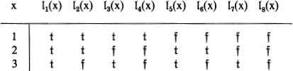
EXAMPLE 1. We give the tables for D = {1, 2} of the term f(f(x)) and of the formula First, we list all possible 1-place functions with values in D (and repeat from § 17 Example 1 the list of 1-place logical functions).⁶⁴

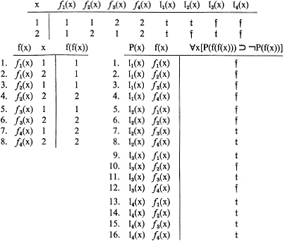
Here is the computation of Line 5 of the table for f(f(x)) (left):

We now compute the entry for Line 7 of the table for the formula (right). This requires us to compute the following supplementary table.

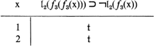
Here are the computations for this supplementary table.¹⁰⁶

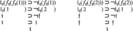
Since the supplementary table has a solid column of ’s, is in Line 7.

The definitions of valid and of valid consequence (again to be abbreviated using “”) are as before (also of .

A little consideration shows that all of the model-theoretic results stated above for the predicate calculus remain good under this extension of the language, where now in THEOREM 15 r can be any term (not just any variable) which is free for x in A(x) in the extension of the earlier notion (§ 18) obtained by calling an occurrence of a term in a formula free if each variable occurrence in it is free in the formula. Thus, briefly, r is free for x in A(x), if no (free) occurrence of a variable in r becomes bound as a result of substituting r for the free x’s in A(x). Similarly, in the definitions preceding THEOREM 17, and in THEOREM 18, r₁ , . . . , r_pi or r₁ , . . . , r_p can be any terms under the conditions stated there for variables.

The proof theory of the predicate calculus with functions differs only by our allowing the r in the ∀-schema and the ∃-schema to be any term free for x in A(x). The corresponding changes can then be made in ∀-elimination and ∃-introduction in THEOREM 21 and in its COROLLARIES.

Now that we are allowing 0-place mesons to name individuals (i.e. members of D), we can use these for “Jane” in (a)-(c) beginning § 16, and for “Socrates” and “five” in Examples 19 and 20 § 26. The only difference this makes from using variables (held constant for the valid consequence and deducibility relationships) as we did in Chapter II is that there we might have used the same variables also in bound occurrences. That would make no trouble for our logical analyses, though it seems unnatural since in ordinary languages we normally use proper nouns etc. for such purposes.

The substantial gain in using functions comes when functions of n > 0 variables are employed in conjunction with the equality predicate (§§ 29, 30).

EXERCISES. 28.1. How many lines does the table have when D = {1,2}? Compute the indicated line.

(a) g(f(g(x, f(h))), x) when f(x), g(x, y), h, x are f₄(x),f₇(x, y), 1, 2, respectively (where f₇(1, 1) = f₇(2, 2) = 1,f₇(1, 2) = f₇(2, 1) = 2).

(b) ∀xP(g(f(g(x, f(h))), x)) ∨ Q, with the above assignment extended by I₂(x), to P(x), Q.

28.2.   Which of the following terms are free for x in the formula ∀w(P(x,y) ∨ ∃zQ(y,x) ⊃ R(w))? (a) x. (b) g(z, f(x, y)). (c) f(x, y). (d) g(w, y). (e) g(y, f(h, x)).

28.3. Fix the proof of Theorem 15 (b) to apply here.

* § 29. Equality. The predicate calculus with equality (or with identity) can be described as arising from the predicate calculus (Chapter II or § 28) by giving one of the 2-place ions a special treatment. We write this ion as “— = —” and read it “— equals —”.

For our model theory, we evaluate x = y by the logical function l(x, y) whose value is when x and y have the same value, and 0 otherwise (e.g. when D = {1, 2}, by I₇(x, y) Example 3 § 17). So in the predicate calculus with equality, the truth tables Are not entered with a value of x = y, as its value is fixed in advance (as are the values of the logical symbols ~, ⊃, &, ∨, ¬, ∀, ∃). In the predicate calculus with equality, by a proper ion we shall mean an ion other than — = —.

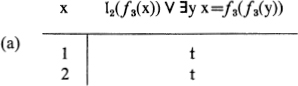
EXAMPLE 2. Here is the truth table for D = {1, 2} of ∀x[P(f(x)) ∨ ∃y x = f(f(y))] (written in two columns to save space).

∀x[P(f(x))∨∃y x = f(f(y))]

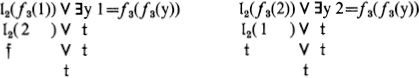
Here is the computation of Line 7.

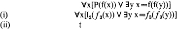
To get (ii), we need the following supplementary table.

The two computations for this are as follows (explained below).

To get the used here in the second line of each column, we need two more supplementary tables:

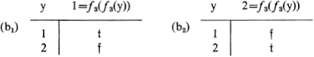
Here are the computations for these.

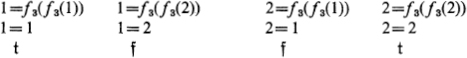
The last step in each of these four computations is by the rule for evaluating = . Since each of (b₁) and (b₂) has a , we get the in the second lines of the two computations for (a) by the rule for evaluating ∃. Then by the rule for ∀ we get (ii).

EXAMPLE 3. Here are the tables for ∃x∀y(P(y) ⊃ x = y) and ∃x[P(x) & ∀y(P(y) ⊃ x = y)] when D = {1,2, 3}. First we list the possible values of P(x) (as in § 17 Example 4).

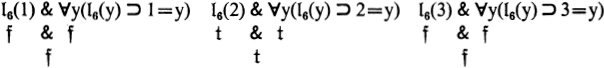
We now compute Line 6 for (a) and (b). We shall need the following supplementary tables.

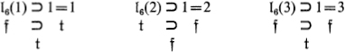
To compute these we need in turn three supplementary tables:

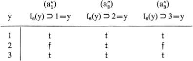
Here are the computations for (a″₁) (and those for (a″₂), (a″₃) are similar):

Using the tables (a″₁)-(a″₃), the evaluation rule for ∀ gives the values shown above in (a′); and those in (b′) are the same thus:

Since (a′) and (b′) each have a , the entry in Line 6 for (a) and (b) is .

Now we note that in Table (a) ∃x∀y(P(y) ⊂ x = y) is for exactly those I(x)′s which have at most one ; and in Table (b)

∃x[P(x) & ∀y(P(y) ⊃ x = y)] is for exactly those I(x)′s which have exactly one . The student should be able to convince himself that this is the case not just for D = {1, 2, 3} but for any (nonempty) D. Thus ∃x∀y(P(y) ⊃ x = y) expresses “there is at most one x such that P(x)” and ∃x[P(x) & ∀y(P(y) ⊃ x=y)] expresses “there is exactly one x such that P(x)” or “there exists a unique x such that P(x)”.

The latter notion is frequently enough used so that we adopt “∃ !xP(x)” as an abbreviation for ∃x[P(x) & ∀y(P(y) ⊃ x = y)]. More generally, “∃!xA(x)” abbreviates ∃x[A(x) & ∀y(A(y) ⊃ x = y)], where in unabbreviating we pick for y a variable free for x in A(x) and distinct from x and the free variables of A(x). (Each two legitimate unabbreviations of “∃ !xA(x)” are congruent, end § 16.) Another useful abbreviation is “x ≠ y” for ¬x = y, or more generally “r ≠ s” for ¬r = s where r and s are any terms.

The results stated above in the model theory of the predicate calculus remain good in the predicate calculus with equality. (Now in § 19, (1) is to be a list of only distinct proper ions including all occurring in E.) We also have further results, which we collect in the following theorem.

THEOREM 28.

(Open equality axioms for =).

(Open equality axioms for a proper ion P(a₁, a₂)).

(Open equality axioms for a meson f(a₁ a₂)).

Similarly, for each n, there are n “open equality axioms” (c₁ⁿ), . . . , (c_nⁿ)for each proper n-place ion P(a₁,. . . , a_n), and n of them (d₁ⁿ), . . ., (d_nⁿ)for each n-place meson f(a₁ . . ., a_n).

PROOFS, (c₁²). By Corollary Theorem 8_Pd=, it will suffice to show that x = y, P(x, a₂) P(y, a₂). So consider any D and any assignment which makes x = y and P(x, a₂) both . Since x = y is , the value of y in the assignment is the same as that of x; so, since P(x, a₂) is , so is P(y, a₂). —

To establish the proof theory of the predicate calculus with equality, we start with the axiom schemata and rules of inference we already have (§ 21, or if functions are allowed § 28), and add as further axioms the formulas shown to be valid in Theorem 28, as we anticipated doing when we called them “open equality axioms”. (The “closed equality axioms” are the closures of the open equality axioms, § 20.) Then by theorem 28, THEOREM 12 and COROLLARY continue to hold.

Now the provability and deducibility results already established for the predicate calculus all hold. This is obvious in the case of the direct rules (as in going from the propositional to the predicate calculus, § 21). Moreover, in the proof of the deduction theorem (§§ 10, 22), applications of the new axioms can be handled under the old Case 3. Then we also have the subsidiary deduction rules based on the deduction theorem which are included among the introduction and elimination rules of THEOREMS 13 and 21.

THEOREM 29.

(Reflexive, symmetric and transitive properties of equality.)

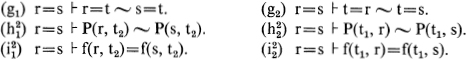
For any terms r, s, t, t₁ t₂, etc.:

Similarly, for each n > 0, we have n such results for each proper n-place ion, and n of them for each n-place meson.

(Special replacement results.)

PROOFS. (For the format (B₁) which we use, cf. §§ 13, 25.) (e) Assume x = y. By (a), x = x. Substituting x for z in (b) (by theorem 21 Corollary 2(c) with Γ empty), x = y ⊃ (x = x ⊃ y = x). Using ⊃-elim. twice, y = x.

Assume r = s. I. Assume P(r, t₂). By substituting r, s, t₂ for x, y, a₂ in , r = s ⊃ (P(r, t₂) ⊃ P(s, t₂)). By ⊃-elim. twice, P(s, t₂). II. Assume P(s, t₂). By substitution in (e), r = s ⊃ s = r. By ⊃-elim., s = r. By substitution in (e), s = r ⊃ (P(s, t₂) ⊃ P(r, t₂)). By ⊃-elim. twice, P(r, t₂).

THEOREM 30. (Replacement theorem.) (I) Let r and s be any terms, t_r be a term containing r as a specified (consecutive) part, and t_s be the result of replacing that part by s. Then:

(II) With r and s as in (I), let C_r be a formula containing r as a specified (consecutive) part (not the variable in a quantifier), C_s be the result of replacing that part by s, and x₁ , . . . , x_q be the variables of r or s which belong to quantifiers in C_r having the specified part within their scopes. Let Γ be a list of (zero or more) formulas not containing any of x₁ , . . . , x_q free. Then:

PROOF, as illustrated next.

EXAMPLE 4. In the following, each of 1-3 after the first is deducible from the preceding, by .

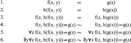
Thus , as (I) asserts.

Each of 1-6 is successively recognizable as being deducible from ∀y f(x, y) = g(x), by ∀-elim., , *71a (since z does not occur free in ∀y f(x, y) = g(x), *72a (since y is not free in ∀y f(x, y)=g(x)). Thus , as (II) asserts.

COROLLARY 1. For C_r, C_s, x₁ ,..., x_q as in (II) of the theorem:

COROLLARY 2. (Replacement property of equality.) Similarly:

Also (α)-(ζ) of § 5 hold now with replacing and “=” replacing “~” and (except in (α)) terms r , s , t , r₀, r₁ r₂,. . . in place of formulas A, B, C, A₀, A_l , A₂, . . . . Hence the chain method applies to equalities (as well as to equivalences) in the predicate calculus with equality. Its usefulness will be illustrated in §§ 38, 39.

THEOREM 31. If E, then there is a proof of E in which there occur no proper ions, and no mesons, not occurring in E.

PROOF. Consider a given proof of E. In this there may occur proper ions, or mesons, not occurring in E. Take the atomic parts (or wholes) of formulas in this proof formed using such ions, and replace them all by ∀xx = x. Then take the terms occurring as parts of formulas in the resulting figure which have such mesons as their outermost symbols and are maximal, i.e. not parts of other such terms, and replace them all by the same variable v not occurring in the given proof. These two operations do not alter the end formula E or any equality axioms for = or proper ions or mesons of E, and they do not spoil any axiom or inference of the predicate calculus (cf. the 2nd paragraph of Footnote 86 §25). However, open equality axioms for ions replaced are altered to x = y ⊃(∀xx = x ⊃ ∀xx = x), and for mesons replaced to x = y ⊃ v = v. But each of these is provable, using ^*1 or (a), and Axiom Schema la. Replacing them by their proofs in the figure last obtained, we have a proof of E using only the proper ions and the mesons occurring in E.

COROLLARY, E in the predicate calculus with equality, if and only if Q₀,. . . Q_s E in the predicate calculus, where Q₀, . . . , Q_s are the closed equality axioms for = and the proper ions and the mesons occurring in E.¹⁰⁷

PROOF. IF. Using ∀-introds. to prove the closed equality axioms Q₀,.. ., Q_s from the respective open ones in the predicate calculus with equality. Only if. Using ∀-elims. to deduce the open equality axioms from the closed in the predicate calculus.

EXERCISES. 29.1. Do the computation for Line 9 in Example 2.

29.2. Write formulas in the predicate calculus with equality to express each of the following.

(a) There are at most two x’s such that P(x).

(b) There are exactly two x’s such that P(x).

(c) The number of x’s such that P(x) is between 2 and 5.

29.3. Establish (b) in Theorem 28, and (f) and (g₁) in Theorem 29. (HINT: for (f), begin with an appropriate substitution into (b).)

29.4. Give a model-theoretic treatment of replacement under equality, paralleling Theorems 19 and 5_Pd (the extension of Theorem 5 in § 19).

* § 30. Equality vs. equivalence, extensionality. We have now (in both model theory and proof theory) the four basic properties of equality: reflexivity ((a) in Theorems 28, 29), symmetry ((e) in Theorem 29), transitivity ((f) in theorem 29) and the replacement property (Corollary 2 Theorem 30).¹⁰⁸

The fourth of these properties, replaceability, is sometimes overlooked in listing the fundamental properties of equality. Model-theoretically, it holds on the basis of our interpretation of “x = y” as meaning that x and y are the same object (Exercise 29.4). We built this interpretation into the rule for evaluating x = y in determining truth tables.

Sometimes “equality” is used in a different sense, so that it possesses only the first three properties (reflexivity, symmetry and transitivity) but lacks the replacement property (except in special contexts). Whatever the terminology and symbolism, it is important to recognize that a relation possessing only the first three properties is not “equality” in the above sense. Such a relation we prefer to call only “equivalence” or “an equivalence relation”.¹⁰⁹

To take an example, consider the set D of all fractions where p and q are integers with q ≠0. Thus D has as members etc. Two such fractions and are equal (i.e. they are the same fraction) exactly if p = r and q = s (i.e. (p, q) and (r, s) are the same pordered pair of integers). However, we are usually not interested in the fractions as fractions but as expressions representing rational numbers.

Now the different fractions etc. all express the same rational number; .... etc. express another; etc. This is sometimes described by saying that we “define equality” between fractions (assuming multiplication and equality of integers already known) by the formula ps = qr. (The student can remember the right member as the result of “cross-multiplying” in the left.)

What objects “ratios” (after Euclid) or “rational numbers” actually are probably does not worry the schoolboy or the layman, provided he gets the “right” rationals in the “right” relationships to one another. Our natural concept of rational numbers seems to be that a rational number is something we get by “abstracting” from the fractions forming a set such as , i.e. by disregarding what is different and keeping what is common. The role of a theory such as we describe next is to show rigorously that a system of objects with the desired properties does exist.

One way to construct these objects is to say that the rational is the set is the set etc. Another way is to pick from each of these classes one particular fraction, say the one in lowest terms with positive denominator, so the fraction is a rational number while ... are expressions for the rational The first method has become fashionable as part of the current practice in classical mathematics of using set-theoretic concepts as the basic vocabulary. We now follow this method in giving a rigorous theory of the rational numbers, supposing such a theory of the integers. . . , —3, —2, —1, 0, 1,2, 3,. .. already established.

While we are giving this theory, in order to remove any possibility of p confusion between a fraction (as a fraction) and the rational number which it represents, we shall write the fractions as ordered pairs (p, q). After the theory has been established, we can revert to writing “ ”, as the schoolboy and the practicing mathematician do; the equations one

ordinarily writes will then read correctly with “ = ” meaning equality between rationals by interpreting the fractions as names for the rationals.

So far we have been tacitly assuming that the set D of the fractions falls into disjoint (i.e. nonoverlapping) nonempty classes D_l, D₂, D₃, . . . , where say D_x = {(1, 2), (5, 10), (-6, -12), . . .},D₂ = {(—1, 3), (5, —15), . . .}, under the criterion that (p, q) and (r, s) belong to the same class exactly if ps — qr in the theory of integers. We should justify this.

First, however, we observe the following: (A) Suppose a nonempty set D is partitioned into disjoint nonempty classes. Then the relation “x and y belong to the same one of the classes”, or in symbols is an equivalence relation, i.e. is reflexive , symmetric and transitive This is so obvious that we can only ask the student to reflect on it a moment.

Now, conversely: (B) If a binary relation with D as its domain is an equivalence relation (i.e. if it is reflexive, symmetric and transitive), then D is partitioned into disjoint nonempty classes such that members x and y of D belong to the same one of the classes exactly when holds.

PROOF. For any member x of D, let x* be the class of all those members u of D such that

I. Because of the reflexive property of , x itself belongs to x*. Thus each of the classes x* for x in D is nonempty, and each member x of D is in at least one of the classes (the classes x* exhaust D).

II. Now consider any members x and y of D. CASE 1: We show that, in this case, x* and y* are the same class (which by I contains both x and y); i.e. each member u of x* is a member of y*, and vice versa. To prove this, first suppose u is a member of x* (in symbols, u ∈ x*), i.e. From the case assumption by the symmetric property of so by the transitive property of , i.e. x* ∈ y*. Similarly, if v ∈ y*, i.e. , then by the case hypothesis and the transitivity, i.e. v ∈ x*. CASE 2: not . this case, x* and y* have no members in common. For, if they had a common member z, then and , and by symmetry and transitivity , contradicting the case hypothesis.

When we start with a set D and an equivalence relation on D to discover the disjoint subsets of D by (B), we call those subsets the equivalence classes of D under the relation .

In particular, when D is the fractions, we can use (B) to conclude that D is partitioned into the disjoint nonempty subsets which we are taking as the rationals. Thus, we define , and verify that this is an equivalence relation (Exercise 30.1 (a)). Then (B) applies.

In going from the fractions to the rationals, we substitute for the domain D of the fractions the new domain D* of its equivalence classes under the equivalence relation just defined. In doing so, the equivalence relation on D becomes, or gives rise to, the equality relation = on D*; i.e. two rationals x* and y* are the same (x* = y*) exactly if, for any (p, q) ∈ x* and (r, s) ∈ y*, .

The reason why we start with the fractions D to build the rationals D* is that the p, q of the fractions (p, q) provide us with the means of defining and performing the operations we wish to perform on the rationals.

Thus, we are accustomed to taking the sum by the following manipulation: (which may be reduced to lowest terms, if we wish). To emphasize that the operation is initially one on fractions as such, we make the definition (p, q) + (r, s) = (ps + qr, qs). But we want an operation on equivalence classes of fractions, since the rationals are those and not the fractions themselves. To confirm that this addition of fractions (p_, q) + (r, s) does give an operation on rationals x* + y*, we must show that the equivalence class to which (ps + qr, qs) belongs depends only on the equivalence classes x* and y* to which (p, q) and (r, s) belong. That is, we need to show that (Exercise 30.1 (b)). For then the addition of equivalence classes x* and y* is defined with a uniquely determined equivalence class z* as result, thus: pick any member (p q) of x* and any member (r, s) of y*; add by the above rule; and take as z* the equivalence class to which the resulting fraction (ps+qr, qs) belongs.

Similarly, we can define the predicate x* < y* between rationals x* and y* by first putting if qs > 0; ps > qr if qs < 0), and then showing that the truth or falsity of (p, q) < (r, j) depends only on the equivalence classes of (p, q) and (r, s) (Exercise 30.1 (d)).

Not all operations on fractions as pairs of integers (p, q) with q ≠ 0 depend only on the equivalence classes to which the fractions belong. E.g. (p, q) ° (r, s) = (p+r, q+s) is a perfectly well defined operation (function) on fractions which does not induce an operation on rationals.

Equivalence (between members of D), unlike equality, does not in general have the replacement property. For example, from (p, q) + (r, s) = (t, u) and (p, q) (p_l, q₁) it does not follow that (p₁ q₁) + (r, s) = (t, u) (though (p_l, q₁) +(r, s) (t, u) follows).

To summarize what has been elaborated on the example of the rationals, if someone has introduced a collection D of objects, and then says “let us define ‘equality’ between these objects”, he is in our terminology proposing to define an equivalence relation. He is not free to define “equality”; the equality relation between the objects is already fixed simultaneously with the introduction of the set D. What he is proposing to define will become equality in the new domain D* consisting of the equivalence classes of D, or in a layman’s terms of the objects that we can abstract or invent by disregarding the differences which in D subsist between members of an equivalence class. —

EXAMPLE 5. We saw in § 29 that expresses “there is a unique x such that P(x)” in the model-theory of the predicate calculus with equality. This cannot be expressed in the model theory of the predicate calculus without equality (Chapter II). To show this, suppose to the contrary we had a formula E of the latter with just one ion P(—) such that E is true when and only when P(x) is evaluated by a logical function l(x) which is for exactly one member of D. Then in particular, E is when D = {1, 2, 3} and P(x) is evaluated by l₆(x) (which has the table f, t, f). Now consider instead a D with four members, say D = {1, 2_l, 2₂, 3}, and let P(x) be evaluated by I(x) where 1(1) = f, I₂(2_l) = I₂(2₂) = t, 1(3) = f. In the new computation, 2₁ and 2₂ behave just as 2 did before, so again E will be t. This contradicts our supposition, since this I(x) is true for two values of x.

As Example 5 illustrates, the rules for evaluation in the model theory of the predicate calculus without equality provide no barrier against splitting any element of any D into a multiplicity of elements which will behave alike in all the computations previously considered. (This process is the reverse of coalescing elements into equivalence classes as new elements.) —

Now we discuss problems of translation from ordinary language into logical symbols when equality may be involved. The basic presupposition for our model-theoretic treatment of equality is that we are dealing with some collection or set as the domain D. This we think of as constituted of “definite well-distinguished objects”.¹¹⁰ So if x is a member of D and y is a member of D, then either x and y are the same member (x = y is true) or x and y are different (distinct) members (x = y is false). In brief, our notion of a domain D already entails the equality predicate over D.

Any application of the predicate calculus, now with equality, is to come after we have a set D as the domain, which we have either constructed or assumed to exist on the basis of supposed facts or for the purpose of the argument. A domain in our sense may constitute quite a sophisticated (or even problematical) abstraction from perceptual experience.

To illustrate, we take the cases of temperature and color. Our sensations of each are fuzzy, so that close temperatures and colors intergrade; it is often hard to say whether two objects under given conditions have the same temperature or color. But physics and psychology have constructed mathematical models, in which temperatures are represented “exactly” by real numbers (≥ an “absolute zero”), and colors by points in some three-dimensional region (or triples of real numbers subject to certain restrictions). In classical mathematics, each two real numbers x and y are either equal or unequal, by the following rule: write each real number as the sum of an integer (positive, zero or negative) and a nonnegative infinite decimal fraction; e.g. π = 3 + .14159.. . = (briefly) 3.14159. . ., 2/3 = 0.66666.. . ; 75/2 = 37.50000 = 37.49999.. ., – 3/4 = – 1 + .25000 = –1 + .24999.. .. Sometimes there will be two ways to do this, one using infinitely repeating 0’s and the other infinitely repeating 9’s; in these cases, let us now choose always the same way, say the one with repeating 9’s. Now x = y if x and y have the same integer-plus-decimal representation; x ≠ y otherwise, i.e. if the integers are different, or the decimals differ in at least one digit.¹¹¹

If one starts with our notion of a domain D, and forms all possible one-place predicates P(x) over D (or simply all possible one-place logical functions l(x) over D),⁶⁷ then x = y can be defined thus: x = y ≡ {for all P, P(x) ~ P{y)}- For, if x and 2 are the same member of A then by our notion of a predicate, for each P, P(x) and P{y) are the same proposition, so P(x) ~ P(y). On the other hand, if x and y are different members of D, then there are predicates P which “separate” them, i.e. such that P(x) is true while P(y) is false or vice versa, so not, for all P, P(x) ~ P(y). This definition expresses the so-called principle of identity of indiscemibles of Leibniz 1685+ (reproduced in Lewis 1918 pp. 373-387): if we can discern no property P in which x and y differ, x and y are identical. In second-order predicate calculus (references in § 17), we can hence regard x = y as an abbreviation for , instead of introducing it as a primitive predicate. Since conceptually the idea of equality underlies our notion of a domain and of predicates over the domain, it seems more elementary and direct to introduce equality as we do than to define it by reference to all predicates. Of course, the Leibniz definition would only be available to us if we were considering second-order logic.

For the Leibniz definition to seem a natural way to introduce the idea of equality (i.e. a way which explains its meaning rather than simply states a necessary and sufficient condition for what is already understood), one must start from a rather different position than in our model theory. For, it requires one to entertain the applicability of properties P to objects x, or to consider the truth or falsity of values P(x) of a predicate, before the objects x themselves are clearly distinguished.

In our theory with a presupposed domain D, whether objects are equal or not is dependent on the picture of the world out of which we have constructed the D.

Is the morning star x equal to (the same as) the evening star y? (In symbols, is x = y?) It is when the domain D** is that of astronomical bodies, wherein both the morning star and the evening star are Mercury (seen at different times). To shepherds, unversed in astronomy, the star observed in the morning, and the star observed in the evening (on other dates) are two different natural phenomena; the domain D* is different. To a child, the evening star seen on one date and the evening star on another date may be different phenomena is still another domain D. We can think of D* as equivalence classes in D, and of D** as equivalence classes in D* (or larger ones in D), where in each case the abstraction results from recognizing different members of one set as related by an equivalence relation or thinking of them as different manifestations of the same “underlying reality”.

The forward implication in Leibniz’ definition of equality, namely that x = y implies ∀P(P(x) ~ P(y)), expresses in a little different way what we called the “replacement property of equality” (Corollary 2 theorem 30). Our principle is stated with respect to the class of formulas under consideration, and includes the case of replacement inside quantifiers. The same property is also sometimes described as “extensionality”, from the standpoint of the contexts in which x = y justifies the replacement of x by y. A context in which such replacement is justified is called extensional, one in which it is not, nonextensional or sometimes intensional. This jibes with our previous use of “extensional” vs. “intensional”, where replacement under “~” was involved.⁹²

Consider the following. “Let n be the number of planets in the solar system. Kepler did not know that n > 6. But n = 9 (according to current science). Therefore Kepler did not know that 9 > 6.”¹¹² The context “Kepler did not know that — > 6” is intensional, since the meaning of what is put in place of the blank, rather than just the value of it as a member of the domain D, affects the truth of the result. So the replacement of “n” by “9” on the basis of the equality “n = 9” is not justified in “Kepler did not know that n > 6”.

By this example, we can add the logic of knowing, believing, etc. to the examples already given end § 12 of nonextensional contexts for replacement under material equivalence, i.e. where equality of truth values is insufficient to justify replacement. For, from “n = 9” we get “n > 6 ~ 9 > 6” by a correct application of replacement (theorem 30 (II)); but “n > 6” cannot be replaced by “9 > 6” in “Kepler did not know that n > 6”.

When a context is not extensional for replacement under equality, something is being taken into account in it that is not recognized in constituting the elements of the domain D. By splitting up those elements to construct a new domain D', the equality in D may become an equivalence relationship on D' while extensionality is restored. Thus if we construe D' as “mental” objects for Kepler rather than “real” objects, so that n and 9 are different mental objects, then “n = 9” is not true. So the occurrence of nonextensional contexts for equality can be regarded as just another way of looking at the difference between an equality and an equivalence relationship. Admittedly, in matters of knowledge or belief, it may be rather hard to describe exactly a domain D’ which suffices to restore extensionality.

Since a shift in our understanding of what the domain D of objects is can make a difference between equality and equivalence, it is not surprising that the terminology is often confused. Here is a table of translations.

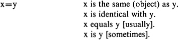
The first two readings are the least ambiguous. But we normally use the reading “equals” for “ = ”, because it is briefer than the first two, and indeed is the standard way of reading “ = ” in mathematics. But mathematicians often use “ = ” and “equals” for what we consider an equivalence relationship. As a new example, textbooks in plane Euclidean geometry often write “AB = CD” to mean that the line segments AB and CD are of the same length. One can’t then replace “AB” by “CD” in “AB EF” (read “AB is perpendicular to EF“). So the translator into our logical symbolism must be on guard to recognize whether “equals” is being used for our = , or for an equivalence relationship. Of course, “length AB = length CD” is an unambiguous translation of “AB = CD” in the present example, and this could be written “AB CD”. Besides equality or identity in the fundamental sense, mathematicians need many (other) equivalence notions. So terms like “equivalent”, “congruent”, “similar”, “homologous” (and as we have seen, sometimes “equal”) are often employed for such equivalence notions.

We come finally to “is” or other forms of the verb “to be”. In addition to its use as an auxiliary verb (“he is going”, “this was done”, “John is loved by Jane”) and in expressing the existential quantifier (“there is”), we need to notice three others. (1) When A and B are objects both considered as members of the same domain D, “A is B” (almost always) means “A = B” in our sense, i.e. that A and B are the same member of D. Examples: “The number of planets is 9”, “Two plus two is four”. (2) When A is an object considered as a member of a domain D, and B is a subset of D, “A is B” means that A is a member of B, and is translated by “A B” or B(A). Examples: “Socrates is a man”, “Snow is white”, “Jane is lovely”. (3) When A and B are both subsets of D, “A is B” means that the subset A is included in (is a subset of) B, and is translated by “A B” or . Examples: “Men are mortal”, “Cats are animals”.

So as not to give away the translation in advance, we have used capital “A” and “B” in all three uses. With symbolism chosen as we have usually chosen it, (l)–(3) would be distinguishable by lower case (small) letters for members of sets and capital letters for sets, thus: (1) “a is b” translated “a = b”. (2) “a is B” translated “a B” or B(a). (3) “A is B” translated “A B” or . (In translation from verbal language the problem is then, “Which terms correspond to small letters, and which to capitals?”)

This usage cannot be preserved if we consider sets whose members are also sets whose members we may want to name. “Men are numerous” should be translated “M N” where M is the set of men and Nis the set of numerous sets.

It should hardly need to be pointed out that confusion of these meanings of “is” can lead to fallacies.

Under Meanings (1) and (3), “is” is transitive and (Barbara, Example 23 §27)); but not under Meaning (2) (fallacious example: “Socrates is a man. Men are numerous. Therefore Socrates is numerous.”).¹¹³ Under (1), “is” is both reflexive and symmetric; under (2), “is” is not symmetric, nor (as set theory is usually understood) reflexive; under (3), “is” is reflexive, but not symmetric.

EXERCISES. 30.1. (a) Show that is an equivalence relation between pairs of integers (p, q) with q ≠ 0. (b) Show that (p, q) + (r, s) = (ps + qr, qs) is an operation depending only on the equivalence classes (cf. the text), (c) Treat similarly (p, q) . (r, s) = (pr, qs). (d) Treat similarly (p, q) < (r, s) as defined in the text.

30.2. Let D = {0, 1,2, 3, 4, 5, 6, 7} and x y = (x–y or y–x is an even natural number). Show that is an equivalence relation on D, and list the equivalence classes.

30.3. Translate into logical symbolism, and establish validity or invalidity.

(a) Everybody loves Jane. Jane loves someone. Therefore there are two people who love each other.

(b) Everybody loves Jane. Jane loves someone besides herself. Therefore there are two people who love each other.

(c) π is the ratio of the circumference of a circle to its diameter, tc is between 3.1415 and 3.1416. Therefore the ratio of the circumference of a circle to its diameter is between 3.1415 and 3.1416.

(d) Samuel Clemens wrote “Huckleberry Finn”. Mark Twain wrote “Huckleberry Finn”. “Huckleberry Finn” is the work of one author. Therefore Mark Twain is Samuel Clemens.

(e) Jane has at most one husband. Jane is married to Thomas. Thomas is thin. William is not thin. Therefore Jane is not married to William.

(f)  Tom is a brother of Dick. Dick is a brother of Harry. No man is his own brother. Therefore Tom and Harry are different people.

(g)* Every person in this room has a brother and a sister both in this room. No person is his own brother or sister. No brother of anyone is a sister of anyone. Therefore there are either no people or at least four

people in this room.

(h) The moon seen today is round. The moon seen twelve days ago was crescent shaped. The moon today and the moon twelve days ago are the same object. Therefore something is both round and crescent shaped.

(i) A rose is red. Red is a color. Therefore a rose is a color.

(j) A gnu is an antelope. An antelope is a mammal. Therefore a gnu is a mammal.

(k) Salt and sugar are white. Nothing is both salt and sugar. Therefore nothing is white.

*§31. Descriptions. To complete our survey of first-order logic (cf. § 17), we shall discuss briefly the definite article “the” and the indefinite article “a” or “an”.

We can name objects by descriptive phrases containing the definite article “the”, such as the following: (a) “the present queen of England”, (b) “the present king of France”, (c) “the sister of a;”, (d) “the father of x”, (e) “the number which added to x gives y”, (f) “the number whose square is x”, (g) “the least common divisor of x and y”, (h) “the third smallest prime number”, (i) “the greatest prime number”, (j) “the number w such that, for all x, x + w = x”. In our model theory, by “objects” we mean members of the domain or universe of discourse D about which we are thinking at the moment.

For some of the objects just named, we have other names not using “the”: (a₁) “Elizabeth II” (1966), (e₁) y – x, (h₁) 5, (j₁) 0. The usefulness of descriptions as a linguistic device is that it gives us a way to make a name, usually for temporary use, when we do not already have one but have the vocabulary to describe or characterize the object.

As our language is commonly understood, a definite description is not used “properly” unless it really does describe a unique object, or, if free variables are present, a unique object for each choice of values of those variables. The general form of a definite description is “the w such that F(w)”. If F(w) is a predicate of just the one variable w, the description is proper exactly if there is just one object w in the domain D such that F(w), this condition translates into our logical symbolism as 3!wF(w) (cf. § 29). If F(w) is a predicate of other variables x₁.. ., x_n as well, write it then also “F(x₁. . ., x_n w)”, then (as long as we are not confining our attention to only certain values of x₁.. ., x_n) the description is proper exactly if, for each x₁. . ., x_n in D, there is a unique w in D such that F(x₁.. ., x_n w); in our symbols, . In this case, the description serves to name a function f(x₁,. . ., x_n) (as well as its values).¹⁰⁵ We include the previous case under this, by allowing n = 0 so an individual (or object) is named.

Since 1848, (b) has been an improper description.¹¹⁴ When D is all persons, (c) is improper, since not every person x has just one sister; only for smaller D’s does (c) define a function f(x). But (d) is proper, though proverbially only a wise x knows the value of f(x). When D is the positive real numbers, (e) is improper (e.g. no positive real number can be added to 5 to give 3), but (f) is proper. When D is all the real numbers, (e) is proper, but (f) is not (e.g. 4 has two square roots, 2 and —2). By a theorem of Euclid, (i) is improper.

In ordinary discourse, improper descriptions hardly occur. If someone speaks about “the w such that F(w)” when there isn’t a unique such w, we usually conclude that he is either confused himself or is attempting to mislead us. We might try to say that any sentence A containing an improper description is simply false. But then we run into the difficulty that and A ⊃ B would also be false by this criterion, whereas (by our truth tables for and ⊃) and A ⊃ B must be true when A is false. Whitehead and Russell 1910 pp. 69-75 (66-71 in the 1925 ed.; also it’s in van Heijenoort 1967) handled this difficulty by requiring the part of a sentence which is declared false because it contains an improper description to be indicated; the truth or falsity of larger parts containing it is then to be determined by the usual rules. There is some awkwardness in this; and the problem of the best way to treat descriptions allowing improper ones is still a subject of research.¹¹⁵ Improper descriptions, and partially defined functions (and in other connections, multiple-valued functions) have some uses in mathematics. However, for the brief treatment we give here, we shall follow common usage in avoiding improper descriptions.

But then we have another difficulty, that what a sentence is (or in our treatment of logic, what a formula is) will not always be determinable immediately from the way it is assembled out of its parts (as in our definitions of “formula” in §§ 1,16, 28, 29), but will depend on validity or provability (or valid consequence or deducibility) results. That is, if A contains a part “the w such that F(w)”, and would be a formula under the definition in § 28 or § 29 if this part were allowed as a term, we shall not know whether to call A a formula until we know whether we have ∃!wF(w).

As the price of abjuring improper descriptions, we shall have to live with this difficulty.¹¹⁶ It will not be very hard to do so, since in ordinary discourse and in mathematics we normally want to use definite descriptions only after we already have ∃!wF(w) or ∀x₁. . . ∀x_n∃!wF(x₁, . . . , x_n, w).

We might introduce descriptions into our symbolism by adding an operator “” (read “the w such that”). This would bind variable occurrences in terms F(x_l, . . . , x_n, w) (and in terms and formulas containing such terms), just as ∀x and ∃x do in formulas.

In our treatment here we shall stay within the notation of the predicate calculus with functions and equality as treated above. The descriptions we want can then be handled simply as introductions of new function symbols f.¹¹⁷ Thus, when we have

we may introduce a new function symbol f with the formula

We may even read f(x₁, . . . , x_n) as “the w such that F(x_l, . . . , x_n, w)” if we wish; but its properties will be given by (ii) with (i). We shall make this explicit in the theorem below. Any finite succession of descriptions, each after the first possibly involving the preceding ones, can thus be provided, without piling up complicated patterns of bound variables in the terms. This is the usual practice in mathematics, except in simple passages.

In this treatment, we lose the advantage that descriptive definitions are self-explanatory, since each time a new function symbol f has been introduced, we have to remember the formula (ii) with which it was introduced. If the function expressed by the symbol is to be used often, we will quickly become used to the symbol f for it, and the notation f(x₁, . . . , x_n) will be more convenient than the more cumbersome F(x₁, . . . , x_n, w). It is in speech and in short written passages that the descriptive operator “the w such that” or “” has a clear advantage over introducing new function symbols. However, for our logical analyses of arguments encountered in ordinary language, it is a simple matter to supply (or imagine supplied) function symbols corresponding to the descriptive names used in the language.

So we are to get the effect of proper (definite) descriptions by a theory for adding new function symbols when it has become known (absolutely or under the assumptions we have made) that the functions are definable descriptively.

We shall give the treatment only in model theory, where it is almost trivial. A proof-theoretic discussion (after Hilbert-Bernays 1934) would be a little too detailed to fit well here.¹¹⁸

THEOREM 32.* Let be any list of zero or more formulas in the predicate calculus with functions and equality, F(x_l, . . . ,x_n, w) be a formula containing free only the distinct variables x₁, . . . , x_n, w (n ≥ 0), f be a function symbol not occurring in any of the formulas and F(x₁, . . . , x_n, w), and C be a formula not containing f. Then :If and , then .

PROOF. Consider any given domain D, and any given assignment in D to just the free variables, ions and mesons in , ∀x₁. . . ∀x_n∃ !wF(x₁, . . . , x_n, w), C which makes all of . We must show that C is also . By the hypothesis that , the formula ∀x₁. . . ∀x_n∃ !wF(x₁ . . . , x_n, w) is . By Example 3 § 29 and the evaluation rule for ∀, hence, for each choice of members x_l, . . . , x_n of D as values of x_l, . . . , x_n, there is a unique member w of D such that F(x_l, . . . , x_n, w) is when w is the value of w. So for this w and x₁, . . . , x_n we can write w = f(x_l, . . . ,x_n) where f is an n-place function with arguments and values in D. But now, if we augment the given assignment by taking f(x_l, . . . , x_n) as value of f(x_l, . . . , x_n, then ∀x₁. . . ∀x_nF(x₁, . . . , x_n, f(x_l . . . , x_n) is . So by the hypothesis that , the formula C is also . This is under the augmented assignment; but since f does not occur in C, the formula C is under the given assignment, as was to be proved. —

The effect of this theorem is that, if ∀x₁. . . ∀x_n∃ !wF(x_l, . . . , x_n, w) is a valid consequence of our assumptions , then to the symbols we are using we can add f(x_l, . . . , x_n) expressing “the w such that F(x₁, . . . x_n, w) is when w is the value of w” and to our assumptions the formula ∀x₁. . . ∀x_nF(x₁, . . . , x_n, f(x_l, . . . , x_n)); any formula C not containing f which is a valid consequence of the augmented assumptions will be a valid consequence of the original assumptions. In the process of recognizing C to be a valid consequence, our reasoning may be helped by the additional assumption ∀x₁. . . ∀x_nF(x₁, . . . , x_n, f(x_l, . . . , x_n)). In fact, there can be a very great gain in efficiency here, through the use of the function symbol f(x₁, . . . , x_n in conjunction with the replacement theorem (theorem 30 § 29).

EXAMPLE 6. Let the formulas be constructed as in § 29 with 1, — — (or also —^-1) as the mesons. In the predicate calculus with equality,

(Exercise 31.2). Hence, by theorem 32 (with theorems 9_Pd= and 12_Pd=),

EXAMPLE 7. In Example 6, (2) does not hold omitting ∀x∃!w xw = l (call it then (2′)). For, the two assumption formulas of (2′) are both and the conclusion is , when D is the rational numbers and 1, xy, 0, 1, 0 are the values of 1, xy, x, y, z. (In effect, xz = yz ⊃ x = y lets us prove 0 = 1 from 0·0 = 1·0 by “dividing by 0”.)

COROLLARY. If , and is consistent in the sense that for no formula A do both and hold, then so is .

Now we observe that theorem 32 and its Corollary hold even with “∃w” in place of “∃!w” (call the theorem then THEOREM 32a). The only difference in the proof is that, for each x₁ , . . . , x_n as values of x₁ , . . . , x_n, the w is not completely determined, but a particular one must be chosen from the class of w’s such that F(x₁ , . . . , x_n, w) is when w is the value of w.¹¹⁹

Theorem 32a justifies the use of “proper indefinite descriptions”, i.e. expressions of the form “a w such that F(x₁ , . . . , x_n, w)” where ∀x₁ . . . ∀x_n∃wF(x₁ , . . . , x_n, w) is available (n ≥ 0).

Extreme care should be used, however, in adopting f(x₁ , . . . , x_n) as a translation of “a w such that F(x₁ , . . . , x_n, w)” in any extended argument. For, with each set of values of x₁ , . . . , x_n, the term f(x₁ ,. . . , x_n) in all its uses under the assumption (ii) has to express the same one of the w’s such that F(x₁, . . . , x_n, w). (This is reflected in the equality axioms for f, § 29.) In ordinary discourse, different uses of “a w such that F(x₁, . . . , x_n, w)” in an extended context are likely to be independent of one another. In fact, uses of “a” or “an” to describe a member of a set are usually so transitory that an adequate translation can be given just using a variable as the name of the object described. Examples: “Socrates is a man” (∃x[s = x & H(x)], or simply H(s) as in Example 19 § 26), “A child needs affection” (∀x[C(x) ⊃ A(x)] as in § 27), “A man was here” (∃x[M(x) & H(x)]).

EXERCISES. 31.1. Prove Corollary Theorem 32.

31.2*. Establish (1) in Example 6.¹²⁰

31.3. Show that

Thus, in operating with a proper description, F(x, w) and f(x) = w are equivalent.

31.4. Criticize the following arguments.

(a) Henry and Jane are brother and sister (F(h, j)). Therefore Jane is the sister of Henry (j = f(h); cf. Exercise 31.3). Henry and Edith are brother and sister (F(h, e)). Therefore Edith is the sister of Henry (e = f(h)). Therefore (by (e) and (f) § 29) Edith and Jane are the same person (e = j).

(b) By the meaning of “the sister of John”, John and the sister of John are brother and sister (F(j, f(j)). Therefore (by ∃-introd.), John has a sister (∃wF(j,w)).

---

¹⁰³ The predicate calculus with equality is an important chapter of logic. But what will be needed in Part II of the book will be repeated or cited piecemeal. So the student who has not time for both can skip this chapter.

¹⁰⁴ We pick the short name “meson” (akin to “atom”, “molecule”, “ion”), without making any pretense that there is an analogy with chemistry or physics.

¹⁰⁵ When the variables are interpreted as expressing members of D, the formulas express propositions,⁵³ and the terms express members of D. However, we have nothing here for terms analogous to the generality interpretation of free variables x_u.. ., x_Q in formulas, by which a formula A can instead express the proposition expressed by ∀′A(§20).

¹⁰⁶ We are saving a step here by using the table for f(f(x)) (above left). But of course it is not necessary first to set up tables for terms occurring in our formula.

₁₀₇ does not contain =, then E in the predicate calculus with equality if and only if E in the predicate calculus. However, this is not as easy to prove (cf. Exercise 52.3 and end Footnote 275 § 55).

¹⁰⁸ Using theorem 12_Pd=, the proof-theoretic results imply like results in model theory.

We might have taken these four properties themselves to establish the proof theory. In deriving the last three, we have followed the tradition in proof theory of starting with as few and simple axioms as possible. This proof-theoretic treatment is due essentially to Hilbert and Bernays 1934 pp. 164 ff.

Another (frequently used) method is to employ the axiom (a) and (instead of our other particular equality axioms) the axiom schema x = y ⊃ (A(x) ⊃ A(y)) where z is any variable, A(z) is any formula, and x and y are any variables (distinct from each other but not necessarily from z) free for z in A(z) (and A(x), A(y) are the results of substituting x, y respectively for the free occurrences of z in A(z)).

¹⁰⁹ We are concerned here with equivalence relations between members of the domain D.

We have already been dealing in §§ 2, 4, 5, 15, etc. with an equivalence relation ~ ("material equivalence") between propositions. There we had not only reflexivity, symmetry and transitivity (*91-*21 in theorem 2, or (p)-(8) in § 5), but also replace-ability in the formulas considered theorems and 23). Nevertheless, we do not consider the relation ~ to be an equality relation between propositions, since under our interpretation different (unequal) propositions can be equivalent (namely, they are when they have equal truth values).⁶⁷

¹¹⁰ Cantor 1895 p. 481. Cantor created the theory of sets between 1874 and 1897. We deal with this in §§ 32-35 of Chapter IV.

¹¹¹ There are other theories of real numbers, equivalent to this but more elegant (for one, cf. IM pp. 30-32). Intuitionists (§ 36) do not accept these theories of real numbers; cf. Heyting 1934, 1956.

¹¹² Kepler, famous for his discovery of the laws of planetary motion, died in 1630. The planets Uranus, Neptune and Pluto were discovered in 1791, 1846 and 1930, respectively.

¹¹³ Example from Suppes 1957 p. 183.

¹¹⁴ Or even since 1830. Louis Phillipe’s title was “King of the French”, not “King of France”.

¹¹⁵ See Scott 1967, where other references are given.

¹¹⁶ This difficulty is slightly disguised in the present treatment [THEOREM 32], since for the predicate calculus with functions and equality we have not yet said anything about limiting the supply of mesons available. But if T be closed formulas which express the axioms of some theory for which only the ions and mesons of T are considered available, then the introduction of f entails an enlargement of the class of formulas which we make only after obtaining ∀x₁ . . . ∀x_n∃ !wF(x₁, . . . , x_n, w).

¹¹⁷ We say “function symbol f” rather than “meson f(—, . . . , —)” since we really have in mind a meson consisting of a single new symbol (a “function symbol f”) with argument places following if n > 0. However, the following treatment can also be read with “meson f(—, . . . , —)” in place of “function symbol f”, so that other convenient notations could be used. In fact, the meson f(—, . . . , —) for a given description could even be F(—, . . . , —, w), provided terms arising from different such mesons successively introduced cannot be confused (and the bound variables w are chosen so that the substitutions performed for x_u .. ., x_n in F(x₁, . . . , x_n, w) are free; cf. IM bottom p. 154).

¹¹⁸ Cf. IM § 74. From our model-theoretic treatment and the Godel completeness THEOREM (§ 52 below), some of the proof-theoretic results will follow (but this will not give them in the elementary way which is desired in proof theory; cf. § 37).

¹¹⁹ The principle that, when ∀x_x ... ∀x_n∃wF(x₁ , . . . , x_n, w) is , we can, for each x₁ , . . . , x_n in D, choose such a w in D as the value of a fixed function f(x₁ , . . . , x_n), is a form of the axiom of choice (§ 35 below).

¹²⁰ In substance the solution is the proof of Til in § 39. (A direct proof of (2) with “h” is only slightly longer. In more complicated examples the gain by using theorem 32 or a proof-theoretic version of it can be greater.)