
The chances are your chances are … awfully good.
From certain remarks in the previous chapter, the reader will have an inkling of the serious shortcomings of the frequentist paradigm. Despite its rigorous mathematical basis, frequentism remains unable to answer some of the most basic questions a person is likely to pose when encountering uncertainty. For example, given a random sample X1, X2,…, Xn, one might ask: What is the probability that the next observation, Xn+1, will be less than 10? Rather remarkably, this very natural type of question is off-limits to the frequentist statistician except in the most trivial of cases. The frequentist can offer only an estimate of the desired probability, without answering the question directly.
The Bayesian paradigm provides an elegant framework for resolving such problems by permitting one to treat all unknown parameters as random variables and thus impose prior probability distributions over them. In the present chapter, I will begin by showing how this approach allows one to make explicit statements about the probability distributions of future observations, and then argue in favor of a “fundamentalist” (or “literalist”) Bayesian approach to generating prior probability distributions. Next, I will introduce the expected-utility principle in a Bayesian context and explain how it leads to a very natural system for making decisions in the presence of uncertainty. Finally, I will show how the Bayesian decision framework is sufficiently powerful to address problems of extreme (Knightian) uncertainty.
Frequentist Shackles
Let us recall the Gaussian parameter-estimation problem from the previous chapter. In that example, we observed a random sample from a Gaussian distribution with unknown mean, m, and known standard deviation, s, and were interested in estimating m. We saw first that this could be done by constructing either a point estimate or an interval estimate and, subsequently, that statements about m could be evaluated using the method of hypothesis testing.
Now suppose that a frequentist statistician were asked the question posed above: What is the probability that the next observation, Xn+1, will be less than 10? Clearly, if he or she were to try to answer this question prior to observing X1, X2,…, Xn, then the probability offered would have to be a function of m, which can be denoted by
Probability Xn+1 Is Less Than 10, Given m.
Since m is unknown, this probability would be unknown as well. However, after observing the random sample, the frequentist could estimate the desired probability by inserting the point estimate of m—that is, the sample mean—obtaining
Probability Xn+l Is Less Than 10, Given m Equals Sample Mean.
Unfortunately, this expression does not provide an answer to the question asked, because it is not the true probability. If the sample mean happens to be close to the actual value of m, then this estimated probability is likely to be close to the true probability. However, it will not be the correct probability unless the sample mean is exactly equal to m, and this cannot be verified except in the trivial case when s equals 0.
In fact, there is only one way to compute the probability that Xn+1 is less than 10 without knowing m exactly, and that is to possess a probability distribution over m. Once such a distribution is available, the desired probability may be expressed as
E[Probability Xn+1 Is Less Than 10, Given m],
where the expected value is taken over the distribution of m. That is, instead of inserting a single estimate of m into
Probability Xn+1 Is Less Than 10, Given m,
one can take an average of all possible values of this expression using the distribution of m. If the distribution of m is provided before the random sample is observed, then it is called a prior distribution; if it is determined after observing the random sample, then it is called a posterior distribution. To obtain the latter distribution from the former, one can use the mathematical equation
This result was first developed by British mathematician Thomas Bayes and was published in 1764, a few years after Bayes’s death.1
Bayesian Liberation
Bayes’s theorem gives its name to the Bayesian (i.e., subjective/judgmental) approach to estimation. Using this approach, all that is needed to answer the question “What is the probability that the next observation, Xn+1, will be less than 10?” is a prior PDF of m. Consistent with the presentation in Chapter 2, this prior PDF may be constructed by some type of (more or less sophisticated) judgment. Although there are different schools of Bayesianism, some of which impose more restrictive forms of judgment than others, I believe that a “fundamentalist” (or “literalist”) viewpoint, requiring the statistician to use those estimates that he or she personally believes are most valid (assuming that they satisfy the basic axioms of mathematical probability; e.g., probabilities must be nonnegative and “add up” to 1), is itself most valid logically.2 At the very least, implementing a belief that beliefs must be implemented is logically consistent.
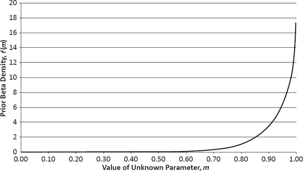
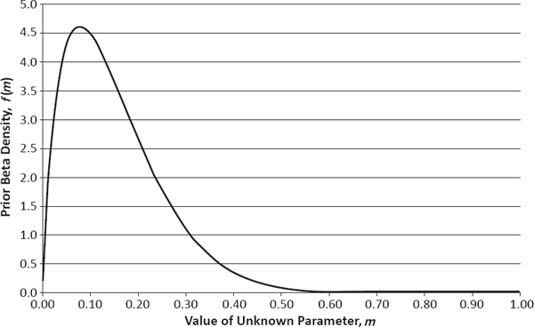
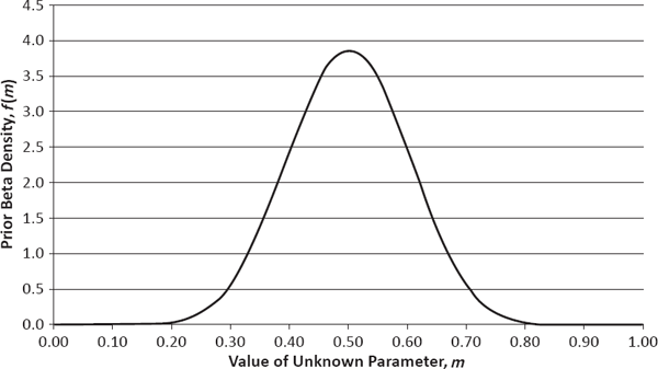
To illustrate how this fundamentalist perspective can be applied in practice, I will consider a number of estimation problems far removed from the capabilities of the frequentist paradigm. In these examples, the parameter m denotes a probability with regard to the state of the world (expressed as the truth of some event or phenomenon) and thus is restricted to values in the interval from 0 to 1 (see Table 5.1). For each event or phenomenon listed in the leftmost column, I offer my prior beliefs regarding this probability, expressed as both a point estimate (in the middle column) and a full probability distribution (in the rightmost column). These probability distributions are from the two-parameter beta family, whose sample space consists of the real numbers from 0 to 1, and each is completely determined by knowing its mean and standard deviation. Their corresponding PDFs are plotted in Figure 5.1.
Prior Probabilities of Various Events or Phenomena

The events and phenomena in Table 5.1 were selected deliberately because they are controversial and likely to be viewed by many as beyond the domain of scientific inquiry. My purpose is to show that if one can provide logically consistent quantitative measures of one’s beliefs in such extremely subjective contexts, then it should be even easier to do so in more mundane matters. Furthermore, as a fundamentalist Bayesian, I would argue that as long as one is capable of formulating such estimates, to refrain from using them—even in the most subjective of contexts—is intellectually dishonest. In short, it is only logically inconsistent beliefs, not crazy beliefs, that are dangerous to science.
Having raised the issue of inconsistency, I think it worthwhile to address a few of the estimates in Table 5.1 that may, at first sight, appear problematic.

Prior PDF of m = Probability Soviets/Cubans Killed J. F. Kennedy

Prior PDF of m = Probability Mobsters Killed J. F. Kennedy

Prior PDF of m = Probability United States Planned 9/11 Attacks
Prior PDF of m = Probability Female Becomes U.S. President or Vice President before 2025
Prior PDF of m = Probability Nuclear Attack Occurs Somewhere before 2025

Prior PDF of m = Probability Alien Intelligence Is Confirmed before 2025

Prior PDF of m = Probability Bigfoot or Yeti Exists

Prior PDF of m = Probability “Face” on Mars Is True Artifact

Prior PDF of m = Probability Life on Mars Exists or Existed

Prior PDF of m = Probability Astrology Has Predictive Value

Prior PDF of m = Probability Clairvoyance Has Predictive Value
Prior PDF of m = Probability Ghosts Exist

Prior PDF of m = Probability Supreme Being Exists

Prior PDF of m = Probability Angels Exist

Prior PDF of m = Probability Afterlife Awaits
In category A (Historical Controversies), for example, I have allocated a probability of 0.55 to the event that President Kennedy was killed by agents of the Soviet Union and/or its Cuban allies and another probability of 0.55 to the event that he was killed by organized criminals. Clearly, these two probabilities sum to a number greater than 1; nevertheless, this does not imply a logical inconsistency because there is a chance that both parties were working together and—more intriguingly—that both parties were working independently and happened to choose the same time and place for their attacks.
Furthermore, in category E (Religion), I have assigned a probability of 0.995 (near certainty) to the existence of an afterlife while according the existence of a supreme being (God) a somewhat lower probability of 0.975. Rather than being inconsistent, these choices simply indicate that I reject the fairly common notion that the existence of heaven (or hell, or purgatory, or whatever) implies the existence of God. To my mind, the existence of God almost certainly implies the existence of an afterlife (although this is clearly not the view of all of the world’s established religions), but I also can imagine the possibility of an afterlife without the existence of a divine entity.
What Is Happiness?
One of the most powerful and important models of human decision making is the expected-utility paradigm.3 This framework, which is widely used in both statistics and economics, does not require a Bayesian setting; however, in conjunction with Bayesianism, it provides a comprehensive and consistent approach to decision making in the face of uncertainty.
The notion of expected utility traces its development to the classical solution of Swiss mathematician Nicholas Bernoulli’s St. Petersburg Paradox. This problem, originally posed in 1713 while Bernoulli held an academic appointment in the eponymous Russian city, contemplates a game in which a fair coin is tossed until it comes up Heads. The player is told that a prize of X units of some currency (e.g., ducats in the original problem) will be awarded, where X equals:
1 if Heads occurs on the first toss;
2 if Heads occurs on the second toss;
4 if Heads occurs on the third toss;
8 if Heads occurs on the fourth toss; and so on;
and then is asked how many units he or she would be willing to pay to play the game.
At Bernoulli’s time, as today, most people would be willing to pay only a very few units to play the game. However, this result was seen as paradoxical by mathematicians of the early eighteenth century because they were accustomed to using expected value as the basic measurement of worth in decisions involving uncertainty. Applying this criterion to the St. Petersburg game yields an expected value of
1 X (1/2) + 2 X (1/4) + 4 X (1/8) + …,
which is infinite. Clearly, there is something puzzling about a game whose expected value is infinite, but which could command only a very small admission fee.
The classical solution to the St. Petersburg puzzle was provided by Daniel Bernoulli (a cousin of Nicholas) in 1738.4 This solution is based upon the observation that most decision makers are characterized by decreasing marginal utility of wealth—that is, a decision maker’s utility (or happiness, as measured in abstract units called utiles) typically increases with each unit of wealth gained, but the incremental increases in utility become progressively smaller as wealth increases.

Natural Logarithm as Utility Function (with Initial Wealth of 10,000)
To determine the true value of the proposed game, one therefore must transform the player’s final wealth, W (that is, the sum of the player’s initial wealth and the random outcome, X) by an increasing and concave downward utility function, U(w), before computing the expected value. D. Bernoulli suggested using the natural-logarithm function, which is depicted in Figure 5.2. Employing this function yields the expected utility

Assuming that the player has an initial wealth of 10,000 units, this expected utility is equal to the utility produced by a fixed award of about 7.62 units. In other words, the expected-utility analysis appears to explain quite well why the game’s actual value is only a few units.
It is important to note that there are a number of sound alternative explanations to the St. Petersburg problem:
• Human concepts of value are bounded above, and thus it is meaningless to speak of a game offering an infinite expected value—or infinite expected utility, for that matter. In fact, Austrian mathematician Karl Menger showed that D. Bernoulli’s solution must be modified by requiring that the utility function be bounded, or else the paradox can be made to reappear for certain payoff schemes.5
• The game lacks credibility, and is in fact unplayable, because no individual or organizational entity is able to fund the arbitrarily large prizes X associated with arbitrarily long streaks of Tails in the coin-tossing sequence.
• Decreasing marginal utility addresses only the impact of the payoff amounts and not the impact of the outcome probabilities. As has been noted by Israeli cognitive scientists Daniel Kahneman and Amos Tversky in their development of cumulative prospect theory, decision makers often misestimate the probabilities of low-frequency events.6 Clearly, this type of effect could substantially lower the perceived expected value of N. Bernoulli’s game.
Interestingly, the third bullet point is consistent with an argument that is often made by my own actuarial science students: that a principal—if not the principal—reason the St. Petersburg game seems unappealing is that it is very difficult to believe that any of the larger values of X will ever be achieved, given that their probabilities are so small. This highly intuitive phenomenon would be especially significant in the context of heavy-tailed outcome distributions, such as those encountered with certain insurance and asset-return risks. It also offers the advantage of not requiring the assumption of decreasing marginal utility, which, while a thoroughly reasonable hypothesis, seems strangely extraneous to problems of decision making under uncertainty.
Given that I interpret my students’ argument correctly, the issue of misestimating the probabilities of low-frequency events can be addressed by positing a simple mathematical model. Specifically, one can assume that every decision maker is characterized by an apprehension function, A(x), rather than (or perhaps in addition to) a utility function, which can be used to create a subjective probability distribution over the random outcome, X, by taking the product of this new function and the true underlying PMF, p(x).
I will assume further that most decision makers are risk pessimistic in the sense that they tend to underestimate the probabilities of large positive outcomes and to overestimate the probabilities of large negative outcomes. This behavior is modeled by requiring that the apprehension function be a positively valued decreasing function that is flat at the expected value of the outcome. In other words, the smaller the outcome, the greater the decision maker’s apprehension concerning that outcome; however, in a neighborhood of the mean outcome—that is, for “typical” values of X—there is very little discernable change in the relative adjustments applied to the PMF. In addition to risk pessimism, it seems reasonable to assume that many decision makers are characterized by what might be called impatience: the property of increasing marginal apprehension below the mean and decreasing marginal apprehension above the mean; in other words, the apprehension function is concave upward below the mean and concave downward above the mean. Figure 5.3 provides a sketch of a hypothetical apprehension function for a risk-pessimistic and impatient decision maker with an expected outcome of 0 units.

Hypothetical Apprehension Function (Characterized by Risk Pessimism and Impatience)
To apply the apprehended-value principle to the St. Petersburg game, first note that the expected outcome is infinite, implying that a risk- pessimistic decision maker with impatience would have an apprehension function resembling only the left-hand portion of the curve in Figure 5.3; that is, A(x) would be decreasing and concave upward. Essentially, this means that the smaller payoffs would be given substantially more weight relative to the larger payoffs, and so, for an appropriate selection of the apprehension function, the apprehended value of N. Bernoulli’s game could be made arbitrarily close to 0.
Risk Versus Uncertainty?
In his influential 1921 treatise, Risk, Uncertainty, and Profit, American economist Frank Knight distinguished between the concepts of risk and uncertainty as follows:7,8
Uncertainty must be taken in a sense radically distinct from the familiar notion of Risk, from which it has never been properly separated. The term “risk”, as loosely used in everyday speech and in economic discussion, really covers two things which, functionally at least, in their causal relations to the phenomena of economic organization, are categorically different…. The essential fact is that “risk” means in some cases a quantity susceptible of measurement, while at other times it is something distinctly not of this character; and there are far-reaching and crucial differences in the bearings of the phenomenon depending on which of the two is really present and operating…. It will appear that a measurable uncertainty, or “risk” proper, as we shall use the term, is so far different from an unmeasurable one that it is not in effect an uncertainty at all. We shall accordingly restrict the term “uncertainty” to cases of the non-quantitive type.
In short, Knight argued that risks are predictable from empirical data using formal statistical methods, whereas uncertainties cannot be predicted because they have no historical precedent. This distinction is often used to explain: (1) uninsurability—that is, the refusal of insurance companies to underwrite certain types of exposures because of anticipated, but actuarially intractable, structural changes in loss distributions (such as those caused by more generous civil justice awards);9 and (2) flights to quality—that is, the abandonment of certain asset or derivative markets by traders perceiving forthcoming, yet unforecastable structural changes in return distributions. In both contexts, the structural changes often are described in terms of potentially unprecedented variations in the tail-heaviness of the relevant probability distributions.
While there certainly exists a qualitative difference between the concepts of predictable risk and Knightian uncertainty, it is not immediately clear why, from a quantitative standpoint, this difference is anything more than a simple distinction between “lesser risk” and “greater risk.” In particular, one might ask: Is it possible to forecast and make decisions regarding such uncertainties using formal statistical methods? To examine this question more closely, let us consider a representative example from insurance underwriting.
One of the insurance industry’s most worrisome lines of business is pollution liability, in which individual losses often are modeled using heavy-tailed probability distributions. For the purpose at hand, let us assume that the total loss amount covered by a particular insurance company’s pollution liability policy, recorded in millions of dollars, is captured by a Pareto random variable, X. As was previously discussed, this random variable possesses an infinite standard deviation if the a parameter is less than or equal to 2 and an infinite mean if a is less than or equal to 1. To make the implications of Knightian uncertainty especially poignant, let us assume further that: (1) throughout the insurance company’s historical experience, the value of a has always remained fixed at 2.5 (for which both the mean and standard deviation are finite); but (2) the insurance company’s actuaries now anticipate a major structural change in civil justice awards that is likely to cause a to shrink dramatically and in a manner without historical precedent.
For the insurance company to continue writing its pollution liability coverage, its actuaries must be able to forecast the random variable X for the post-change period and also to estimate an associated decision-making criterion, such as the company’s expected utility. If the actuaries are frequentist statisticians, then they must estimate a with some value â in the interval from 0 to 2.5 to compute
Expected Utility of (Initial Wealth + Premiums–X), Given â;
whereas if they are Bayesian statisticians, then they must provide a probability distribution over a on the sample space from 0 to 2.5 to compute
E[Expected Utility of (Initial Wealth + Premiums–X), Given a].
Interestingly, it is not the computational differences between the frequentist and Bayesian approaches that are most critical in the context of Knightian uncertainty. Rather, it is the fact that frequentist actuaries would be entirely unable to construct â because they have no formal procedure for saying anything about a in the absence of relevant historical data, whereas Bayesian actuaries would have no trouble positing a probability distribution for a because they are used to selecting prior distributions based largely—and sometimes entirely—upon judgment. Note further that, even in extreme cases in which such a prior distribution places substantial weight on values of a less than 2 (for which the standard deviation and possibly even mean are infinite), there is no obstacle to calculating the expected utility as long as the utility function is bounded.10 Thus, the qualitative difference between risk and Knightian uncertainty poses a quantitative conundrum for frequentists, but not for Bayesians.
It is rather instructive to note that insurance actuaries often use Bayesian methods precisely because of data limitations and the necessity of incorporating human judgment into the decision-making process.11 Therefore, in the context of the present discussion, one actually could argue that Bayesian methods are not only resistant to issues of Knightian uncertainty, but also specifically motivated by, and designed to resolve, such issues.
This leads to an interesting question: To a Bayesian, is Knight’s distinction between risk and uncertainty ever of real significance? Somewhat surprisingly, I would argue that it is. Specifically, Knight’s use of the terms measurable and unmeasurable to distinguish between risk and uncertainty, respectively, is quite valid in a Pickwickian sense.
Although Knight employed unmeasurable to mean a random outcome without historical precedent, a similar term—nonmeasurable—is used in probability theory to describe a mathematical set that cannot be used as the sample space of a proper random variable (because there is no way to distribute probability in a nontrivial way across such a space). Consequently, if one were to contemplate a random outcome a that must take values from a nonmeasurable set, then not even the most fundamentalist Bayesian could construct a legitimate prior distribution for a, and further analysis would be impossible.
Fortunately, such problems have not (yet) arisen in insurance or financial markets, or other quotidian realms of human activity, where conventional discrete and/or continuous sample spaces appear quite sufficient. However, things are not so clear-cut at the epistemological edge of human speculation. For example, as I will argue in Chapter 12, related issues actually do arise in attempting to place a prior distribution over all possible configurations of an infinite set of explanatory variables in a statistical-modeling setting.
Non-Expected-Utility Theory
At the end of Chapter 2, I noted that there exist alternative theories of probability that will not be considered in this book because I find them insufficiently intuitive. I now wish to make a similar point regarding alternatives to the expected-utility paradigm. Although it is true that one alternative to expected utility (i.e., apprehended value) already has been considered, my purpose in that case was primarily to show that sometimes a simple intuitive model may offer as good an explanation as a classically accepted model. I thus will make no attempt to address the vast field of academic inquiry that goes by the name of non-expected-utility theory, except to point out below the sort of weaknesses that it is intended to address.
One of the most compelling arguments against the expected-utility framework was presented by French economist Maurice Allais in 1953 and is often called the Allais paradox.12 In this problem, a decision maker is given the following two choices:

Essentially, Choice 2 is the same as Choice 1, except that $1,000,000 is subtracted from each of the items in Choice 1 with probability 0.89 to obtain the corresponding items in Choice 2. Therefore, according to the expected-utility criterion, anyone who prefers A1 to B1 in Choice 1 also should prefer A2 to B2 in Choice 2, and vice versa. However, experimental evidence shows that in practice, most people prefer A1 to B1 (presumably because they like the idea of gaining $1,000,000 with certainty, and do not want to accept even a 0.01 chance of getting $0 in return for a potential outcome of $5,000,000) and B2 to A2 (presumably because the 0.01 increase in the chance of getting $0 is not very significant when there is already a 0.89 chance of getting $0, and so it is worth taking this chance in return for the $5,000,000 potential).
So is this a failure of expected utility? Certainly, the experimental evidence discredits the descriptive value of the theory—that is, its value as a positive-economic model of what people actually do in certain circumstances. However, I would argue that there is no reason to believe that such evidence undermines the prescriptive value of the theory—that is, its value as a normative-economic model of what people should do in certain circumstances.
To a large extent, I agree with the assessment of American (Bayesian) statistician Leonard Savage, who, having selected inconsistent responses when first presented with Allais’s problem, determined that he had simply made an irrational choice and that further thought enabled him to reconcile his two choices.13 In my own case, I certainly would have selected A1 over B1 and B2 over A2 when I first saw the Allais problem some years ago, but now would choose B1 over A1 and B2 over A2. The principal reason for this change is that the potential regret that could arise from getting $0 after choosing B1 over A1 now strikes me as a somewhat irrational psychological concern that I would like to eliminate from my own decision making if possible. In summary, then, I find the Bayesian expected-utility worldview a comprehensive and cogent framework for prescriptive decision making.
ACT 1, SCENE 5
[A spacious and well-appointed office. Middle-aged man sits at large wooden desk; Grim Reaper approaches quietly.]
REAPER: Good afternoon, Mr. Wiley. I’m the Grim Reaper. Do you remember me?
MAN: Why yes, of course I do. How long has it been, Reaper? Twenty-five years? Thirty years?
REAPER: It’s been a little more than thirty-three years.
MAN: Well, I can’t say that I’m pleased to see you again so soon. But I would’ve been even less pleased to see you sooner. I guess you finally succeeded in making one of your free throws. How many tries did it actually take?
REAPER: If you must know, it was something over 17 million.
MAN: I see. Well, 17 million is a large number, but it’s nothing compared to infinity. In the great scheme of things, I’d say you did relatively well.
REAPER: Yes, of course you’re right. And you also seem to have done quite well for yourself.
MAN: [Looks around office modestly.] I can’t complain. Professional statisticians are in great demand these days.
REAPER: [Sighs.] And no one demands you more than I.
MAN: Well, then, shall we go?
REAPER: [Unenthusiastically.] Yes, I suppose so.
MAN: Reaper, you don’t seem your old self. I hope there are no hard feelings between us. If it would make you feel better, I’d be happy to offer another challenge: “double or nothing,” so to speak. What I mean is, if I win, you don’t come back for another thirty-three years, but if you win, I have to gather up one of your victims for you—say, a heartbreaking case, an innocent child, perhaps.
REAPER: [Eyes light up.] Really, would you? It would be somewhat irregular, of course. But I’d relish the chance to get even. What do you propose?
MAN: [Smiles, takes out two pieces of paper and two letter-sized envelopes.] OK, here’s the challenge: I’m going to choose a positive real number, and write it down on one of these two pieces of paper without letting you see what it is. Let’s call that number X. I’m then going to toss a fair coin and allow you to see the outcome: Heads or Tails. If the coin comes up Heads, I’m going to write 2 x X on the other piece of paper—without letting you see it, of course; but if it comes up Tails, I’m going to write (1/2) x X on the other piece of paper—again without letting you see it. I’m then going to seal the two pieces of paper in the two separate envelopes, mix them up behind my back, and return them to my desk. You will get to choose one of the envelopes, open it, and look at the number inside. Given this number, you will have to tell me whether, on the average, the number in the other envelope is greater than, less than, or equal to the one you have just seen.
REAPER: How appropriate. Another problem involving averages. Well, I’m certainly up for that. Let’s proceed.
[Man writes down first number, tosses coin (which comes up Heads), writes down second number, seals both numbers in envelopes, mixes up envelopes and returns them to desk. Grim Reaper chooses envelope and opens it to reveal “1”.]
REAPER: OK. This is easy. Since your coin came up Heads, the number in my envelope must be either X or 2xX. It doesn’t matter what number I actually observed that number to be—in this case, it happened to be 1—because, by symmetry, either envelope is equally likely to contain the smaller number, X. Therefore, on the average, the number in the other envelope must be exactly equal to the number in my envelope.
MAN: Are you sure about that?
REAPER: Quite sure.
MAN: Good. Now let’s look at things another way. As you noted, since my coin came up Heads, the number in your envelope must be either X or 2XX. If X equals 1, then the other number must be 2, but if 2X X equals 1, then the other number must be 1/2. Therefore if, after observing the number 1, we determine that that 1 is equally likely to be either X or 2XX, then the expected value of the other number is 2 X (1/2) + (1/2) X (1/2), which equals 1.5. But that, on the average, is greater than the 1 you observed.
REAPER: [Nervously.] But both conclusions can’t be right—
MAN: Correct. Your error was in assuming that any number you observed was equally likely to be either X or 2XX. For any particular number observed—say, the number 1—we can make that assumption. But if that assumption is made for all numbers that could be observed, then we find that our original X has to be chosen from a uniform distribution over the set of all positive real numbers—and that simply can’t be done.
REAPER: Damn! Double damn!
MAN: Yes; it’s certainly one or the other.