Let us suppose for example that some one jots down a quantity of points upon a sheet of paper helter skelter … ; now I say that it is possible to find a geometrical line whose concept shall be uniform and constant, that is, in accordance with a certain formula, and which line at the same time shall pass through all of those points, and in the same order in which the hand jotted them down.
When told that a particular scientific question is theoretically unanswerable, one’s initial disbelief and intellectual rebellion is likely to be followed by wonder and even a certain degree of contentment. Results such as Heisenberg’s uncertainty principle or Chaitin’s impossibility theorem are not only intriguingly counterintuitive, but also psychologically comforting in that they tell us we have reached the end of one particular road of inquiry, and so can begin another. However, when one is told that a question is unanswerable in practice because of shortcomings with empirical methodologies, there is typically more annoyance than awe. This is because we know, or at least strongly suspect, that if we—or someone else—tried just a little harder or spent just a little more time or money, then the epistemological obstacle could be overcome.
In the previous chapter, I discussed the epistemology of randomness in theoretical terms. Given that the species of practice are generally more extensive than the genera of theory, a similar discussion of the bounds of uncertainty in practical, empirical terms will require three chapters in all. The present chapter will address fundamental problems of separating signals from noise in modeling risk-related phenomena. I then will move on to issues of data availability in Chapter 13, followed by the overall paradigm of the scientific method in Chapter 14.
Scholarly Pareidolia?
Sound empirical scientific research begins with the observation and subsequent investigation of patterns in data.2 Fortunately, the human brain is well equipped for this task. Unfortunately, however, it is somewhat overequipped, possessing a well-known proclivity to do its best to make sense out of visual stimuli, regardless of how confusing or ambiguous they may be. This persistent tendency forms the basis for many common optical illusions (such as two-dimensional drawings of cubes that seem to switch back and forth between alternate orientations), as well as the phenomenon of pareidolia, in which a person believes that he or she sees systematic patterns in disordered and possibly entirely random data.
Rather ironically, the line between the overidentification and underidentification of patterns is one pattern that tends to be underidentified. In addition to dubious uses of data in pseudoscientific pursuits such as numerology and astrology, there also are various quasi-scientific methods, such as the Elliott wave principle employed by some financial analysts and neurolinguistic programming methods of business managers and communication facilitators that haunt the boundary of the scientific and the fanciful.
One context in which pareidolia is frequently cited is the field of planetary science, in which sober authorities often warn lay enthusiasts of the dangers of imagining structures from ancient alien civilizations on the surface of the Moon or Mars. Probably the most celebrated example is the “Face on Mars,” an irregularly shaped plateau in the Cydonia region of the Red Planet that, in certain photographs taken from the Viking 1 and Viking 2 space probes, does look remarkably similar to a human face. (Unfortunately, in other photographs it looks much like a natural geological formation, which is why, in Chapter 5, I stated my personal belief that the probability this structure is the creation of an ancient civilization is less than 1 percent.)
Despite my own skepticism regarding the Martian “Face” as an alien artifact, I do think space scientists should be a bit more tolerant of those who imagine intriguing patterns where none may exist. After all, the history of astronomy owes several large debts to this phenomenon, including: (1) the naming of various (entirely imaginary) constellations by the ancients, which today provides a convenient system of locating objects in the celestial sphere; (2) the Titius-Bode law of exponentially increasing distances between the successive planets of our solar system, which spurred the search for new planetary bodies in the late eighteenth and early nineteenth centuries; and (3) the misguided claims (and detailed drawings) of “canals” on Mars, which stimulated interest and funding for the field of observational astronomy in the late nineteenth and early twentieth centuries.
The Titius-Bode law (TBL) deserves particular attention because of its remarkable similarity to the Gompertz-Makeham law (GML) of human mortality, mentioned previously. Taken together, these two principles provide a fertile basis for considering how formal models arise from empirical data and the extent to which they should be trusted.
Some Exponential Patterns
The TBL was proposed by German astronomer Johann Titius in 1766 and subsequently popularized by his compatriot, astronomer Johann Bode.3 It asserts that the average distance from the sun to the orbit of the xth planet in our solar system is given by a linear combination of a constant term and an exponentially increasing function of x.4,5 Beginning several decades later, the GML was developed in two stages. First, British mathematician Benjamin Gompertz noted that the human mortality hazard rate tends to increase exponentially as a function of age (see Figure 1.2), and he therefore proposed a purely exponential hazard curve in 1825.6 Subsequently, British actuary William Makeham generalized Gompertz’s model in 1860, writing the mortality hazard rate at age x as the linear combination of a constant term and an exponentially increasing function of x (i.e., a functional form identical to that of the TBL).7
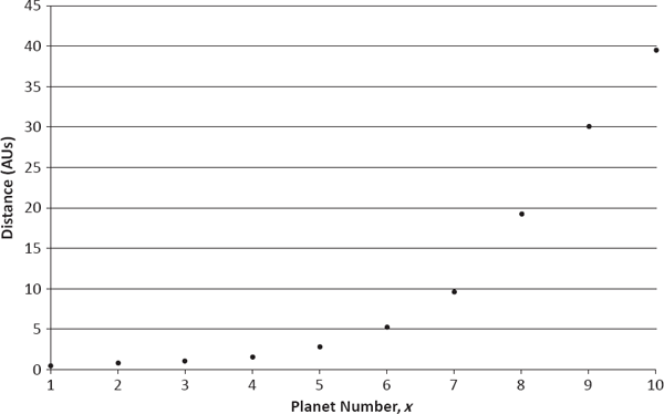
Figures 12.1 and 12.2 present relevant data for the TBL and GML, respectively. In the latter plot, I use the U.S. female (rather than male) population’s mortality hazard rates because of their smoother behavior between the ages of 10 and 35. I also provide hazard rates only at ten equally spaced ages (10, 20,…, 100) to correspond visually to the ten planets of the solar system in Figure 12.1.8,9

Average Planetary-Orbit Distances from Sun (Mercury = 1,…, Ceres = 5,…, Pluto = 10)
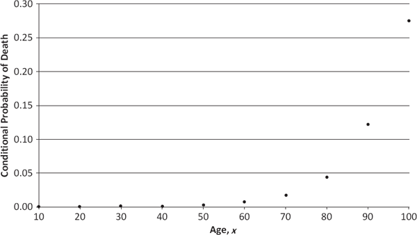
One-Year Mortality Hazard Rate (U.S. Females) Source: Commissioners Standard Ordinary (CSO) Mortality Tables (2001).
The role of the TBL in the history of astronomy is intriguing, both for its motivation of the search for new planets and for the irony that surrounds its actual application. When first proposed, the law fit the orbits of the known planets—Mercury, Venus, Earth, Mars, Jupiter, and Saturn—quite well, and both Titius and Bode noted the conspicuous absence of a planetary body at the distance of the asteroid belt. However, the first object to be discovered after publication of the law was not one of the major asteroids, but rather the planet Uranus (by British astronomer William Herschel in 1781). Although this new planet’s orbit followed the TBL fairly closely, it had not been predicted explicitly by either Titius or Bode (presumably because it fell outside, rather than within, the orbits of the known planets).
Having noted that the orbit of Uranus was approximated well by the law, Bode and others called for a cooperative effort among European astronomers to search the zodiac systematically for the “missing” planet at the distance of the asteroid belt. However, in a strange twist of fate, the first and largest of the asteroids—Ceres—was discovered by Italian astronomer Giuseppe Piazzi in 1801 independently of this effort. Thus, although the law theoretically could have guided both Herschel and Piazzi in their discoveries, it in fact did not. The law did, however, gain much credence among astronomers because of its apparent accuracy and certainly helped spur the search for additional planets. Unfortunately, the next two planets to be discovered—Neptune (in 1846) and Pluto (in 1930)—did not fit the TBL very well, so the law has fallen into general disfavor.
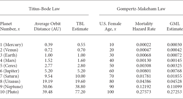
The successes and failures of the TBL are quite evident from Table 12.1, where its accuracy is explicitly compared with that of the GML based upon data from Figures 12.1 and 12.2. Using the error ratio
|(Actual Value)–(Estimated Value)|/(Estimated Value),
it can be shown that exactly three of the mortality hazard rates—those at the end of the first, second, and fourth decades of life—and exactly three of the planetary orbits—those of Mercury, Neptune, and Pluto—deviate from their estimates by more than 10 percent.10 Thus, according to this simple analysis, both laws fit their associated data approximately equally well.
So what is one to make of the two mathematical “laws” displayed in Table 12.1? Do they represent good science or simply good imagination? The answer, I would suggest, is not that simple or clear-cut.
Comparison of Titius-Bode and Gompertz-Makeham Laws
Exponential patterns like those in Figures 12.1 and 12.2 occur frequently in nature, often as the result of obvious underlying physical principles. (For example, it is common to find a population of bacteria growing exponentially because the rate of increase in the population is directly proportional to the population’s current size.) Unfortunately, in the cases of the TBL and the GML, the observed exponential patterns are not justified by any simple underlying theory. Nevertheless, the tentative assumption of an exponential model constitutes a reasonable starting point for further investigation.
The practical question of greatest importance is how long one should retain the exponential model in the presence of contradictory evidence (e.g., the inaccurate estimates in Table 12.1). This problem—of when to switch or update hypotheses—represents a fundamental step in the scientific method. Suppose, for example, that the inaccuracies in Table 12.1 cause formal statistical hypothesis tests to reject both the TBL and the GML. In that case, the conventional decision would be to abandon those models. However, if one’s prior belief in the exponential patterns were sufficiently strong—as formalized in a Bayesian framework—then an appropriate alternative might be to retain the models with certain necessary adjustments.
From Chapter 1, we recall that from ages 10 through 34, young Americans are exposed to fairly dramatic accident and homicide rates. Given how easily that age group can be distinguished from others, it would seem reasonable to believe that the GML provides an accurate reflection of human mortality hazard rates for “normal” populations, but requires one or more additional parameters to account for the accident and homicide pathologies of the U.S. population. A similar approach could be taken with the TBL, for which it might be argued that the proximity of Neptune’s and Pluto’s orbits, as well as the high eccentricity of Pluto’s orbit, suggest that some cataclysmic event millions of years ago caused those two planets to deviate from the “natural” exponential pattern. Again, one or more additional parameters could be added to account for this anomaly.
Some Sinusoidal Patterns
For a more up-to-date example of possible scholarly pareidolia, let us turn to a characteristic of property-liability insurance markets commonly known as the “underwriting cycle.” Addressed in the actuarial literature at least as early as the 1960s, this term refers to the apparently sinusoidal (i.e., sine-function-like) behavior of insurance company profitability data over time and is well represented by the combined ratio data of Figure 12.3.11
Cyclical behavior in insurance profitability is somewhat puzzling to insurance scholars because it belies theories of rational economic decision making, under which any sort of truly periodic behavior in financial markets should be anticipated—and thereby eliminated—by various market participants. For example, suppose that the year is 1975 and that one knows, because of the periodicity of underwriting results, that insurance companies are about to embark on an epoch of increased profitability. Then, as a rational actor, one should decide to benefit from this trend by investing heavily in insurance company stocks. If a substantial number of investors behave in this rational manner, then the insurance industry will realize a sudden influx of capital, which will permit it to expand its writings of insurance and/or to lower premiums. Lower premiums will mean, of course, higher combined ratios (and less profitability per dollar invested), which then will offset the anticipated increase in profitability. Hence, in equilibrium, there should be no cyclical behavior.
Over the past three to four decades, dozens of published research papers have attempted to explain the insurance market’s failure to achieve the sort of equilibrium expected by economists. The most important classes of theories put forward to explain the cyclical pattern in underwriting results are based upon:
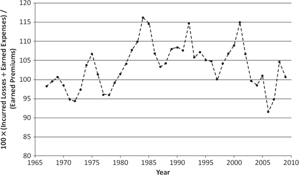
U.S. Property-Liability Combined Ratios (All Industries) Source: A. M. Best Company (2010).
• The influence of prevailing interest rates on markets. For example, an increase in interest rates will encourage insurance companies to lower premiums (per exposure unit) in order to generate more writings (and thus more dollars in total to be invested at the higher rate of return). This will cause the combined ratio to decrease in the short run. However, as losses from the companies’ expanded business begin to come due, they will be disproportionately large compared to premiums, so the combined ratio will increase, eventually passing its original level. Companies then will have to raise premiums (per exposure unit) in order to bring the combined ratio back down again.
• The presence of significant lags between recording losses and setting premiums. For example, assume insurance companies set Year 2’s premiums according to the trend between Year O’s combined ratio and Year 1’s combined ratio and that a substantial increase in the frequency and/or severity of losses occurs between Year 0 and Year 1, but there is no further change between Year 1 and Year 2. This will make Year 1’s combined ratio larger than Year O’s and cause the companies to raise premiums (per exposure unit) in Year 2. Consequently, the companies eventually will find that Year 2’s combined ratio is smaller than Year 1’s, causing them to lower premiums (per exposure unit) in Year 3. This will make Year 3’s combined ratio larger than Year 2’s, and the pattern of raising and lowering premiums (per exposure unit) will continue.
• The impact of major catastrophes or other costly events. For example, if insurance companies must pay a large number of claims as the result of a destructive hurricane, then the combined ratio will increase substantially in the short run. To remain financially solvent, companies will have to raise premiums (per exposure unit), which will cause the combined ratio to decrease beyond its pre-hurricane level. Finally, competitive pressures will force companies to lower premiums (per exposure unit), raising the combined ratio once again.
One major difference between the statistical analyses needed to test the above theories and those needed to test the exponential patterns of the TBL and the GML is that the former require the incorporation of additional variables (such as interest rates, frequency and severity trends, and catastrophe losses) into the respective models, whereas the TBL can be tested by studying orbit distances simply as a function of planet number, and the GML can be tested by studying mortality hazard rates simply as a function of age. Both types of analyses involve observational studies, in which the researcher must rely on the data as they are collected, without the option of generating new observations according to some experimental design. However, the former are infinitely more complicated in that they open the door to arbitrarily large numbers of additional explanatory variables in attempting to assess causality, whereas the latter simply address the presence of a simple functional relationship.
In the next section, I will argue that observational studies are entirely useless for resolving matters of causal relationship, so that such studies can never select convincingly among the three major explanations for cyclical profitability listed above. For this reason, it is particularly ironic that over a period of several decades, researchers pursued causal explanations of the cyclical nature of insurance company profitability without first having carried out a formal test of this pattern. In other words, the preconception of a fundamental sinusoidal relationship was so strong among scholars that they felt it unnecessary to test the simple functional relationship between profitability and time before embarking on more extensive—and unavoidably inconclusive—investigations.
Rather remarkably, when Italian risk theorist and insurance economist Emilio Venezian proposed a formal statistical test of cyclicality in 2006, he found that, on the whole, the statistical evidence for true cyclicality was fairly weak. Specifically, for any fixed time period, at most three out of eight individual U.S. property-liability lines manifested statistically significant profitability cycles at the 5 percent level.12 Thus, it would seem that modern-day scholars are no more immune to the temptations of pareidolia than their predecessors. However, that is not necessarily a bad thing. Although potentially misleading if retained for too long, the identification and use of simple patterns can serve as a coarse data-analytic technique to be replaced by more sophisticated alternatives later in the research process.
Confounding Variables
To explore the fundamental inferential differences between observational studies, on the one hand, and randomized controlled studies, on the other, let us consider the following research question: Are hybrid automobiles more likely than conventional automobiles to have collisions with pedestrians and bicyclists?13 The underlying theory to support such an idea is that hybrids, with dual propulsion systems—one of which is an electric mode that is quieter than the internal combustion engine—are less likely to provide an audible warning of their approach to pedestrians and bicyclists.
A well-publicized observational study conducted by the National Highway Traffic Safety Administration (NHTSA) in 2009 suggested that the answer to this question was “Yes.”14
Among the study’s various summary statistics, the most important were the proportions of pedestrian and bicyclist collisions among total collisions experienced by hybrid automobiles (to be denoted by hPED and hBIC, respectively) during low-speed maneuvers, and the proportions of pedestrian and bicyclist collisions among total collisions experienced by conventional automobiles (similarly denoted by cPED and cBIC) during comparable maneuvers.
These proportions are shown in Table 12.2, along with the associated p-values from testing the null hypotheses: H0: E[hPED] = E[cPED] and (2) H0: E[hBIC] = E[cBIC] . Given the rather small p-values in the rightmost column, the NHTSA concluded that hybrid automobiles do appear to pose additional hazards to pedestrians and bicyclists.
Without rendering judgment on whether or not the NHTSA’s conclusion correctly represents the true state of affairs (which I suspect it does), I would assert that the study was useless for the purposes intended. This is because it failed to recognize the presence of numerous potential confounding variables associated with driver behavior—rather than automobile propulsion systems alone—of which the following are rather conspicuous:
Proportions of Pedestrian and Bicyclist Collisions for Hybrid and Conventional Automobiles During Low-Speed Maneuvers

1. The possibility that as more environmentally conscious individuals, hybrid drivers are more likely to live in neighborhoods with high concentrations of pedestrians and bicyclists.
2. The possibility that because of the physical configurations of their automobiles (especially windows), hybrid drivers pay less attention to relatively small objects, such as pedestrians and bicyclists.
3. The possibility that because of the generally smaller sizes of their automobiles, hybrid drivers tend to avoid more dangerous roadways where collisions with other automobiles, but not pedestrians and bicyclists, are likely.
In other words, since the NHTSA’s researchers did not address these behavioral possibilities, it could be argued that any one of them explains the results of the study just as well as the hypothesis that quieter motors—or any other purely physical characteristic of hybrid autmobiles—make them more dangerous to pedestrians and bicyclists.
Of course, defenders of the observational study methodology could argue that the NHTSA’s researchers were simply remiss in their work and failed to carry out all necessary due diligence in eliminating various confounding variables. For example, the researchers could have controlled for the effects of items one through three by pursuing further studies to determine whether: (1) pedestrian/bicycle density is positively correlated with hybrid automobile density; (2) hybrid automobile windows are smaller and/or create more distortion than conventional automobile windows; and (3) hybrid automobiles tend to be driven less on more dangerous roads. Possibly, negative findings in each of these three additional studies would take care of items one through three. But what can be done about the potentially vast number of less-conspicuous behavioral confounding variables? For example, consider:
4. The possibility that as more cautious people, conventional drivers are more likely to drive carefully in residential neighborhoods (where concentrations of pedestrians and bicyclists are greater).
5. The possibility that as more technologically savvy people, hybrid drivers are more likely to be distracted by mobile phones and other electronic devices while driving at low speeds (i.e., in residential neighborhoods).
6. The possibility that as more self-consciously altruistic people, hybrid drivers are more likely to feel entitled to drive fast in residential neighborhoods.
One could go on and on, simply by suggesting behavioral factors that could be either positively correlated with both hybrid ownership and colliding with a higher proportion of pedestrians/bicyclists or negatively correlated with both hybrid ownership and colliding with pedestrians/bicyclists. To erase any doubts that this list can be made quite vast, consider that the total number of protein-encoding human genes, M, is currently estimated to be somewhere between 20,000 and 25,000. Denoting these genes by the sequence G1, G2,..., GM, one can easily introduce M potentially confounding variables of the form:
The possibility that gene Gi is responsible for traits that make an individual both more likely to purchase a hybrid vehicle and more likely to collide with pedestrians/bicyclists.
If this number is still unsatisfactorily small, then one can look at the truly infinite array of potential environmental factors: exposure to alcohol during gestation, distress at birth, birth order, use of breast- vs. bottle-feeding, parental disciplinary system, family wealth, quality of education, exposure to toxins, etc. Obviously, the NHTSA’s researchers could not control for all of these effects because it is impossible to do so in any finite amount of time.
To clarify how a randomized controlled study would avoid the problem of behavioral confounding variables, consider the following experimental design:
• First, the researchers select a large number of individuals—perhaps 10,000—at random from the U.S. population and divide them randomly into two equal-sized groups, H and C.
• Next, each driver in group H is given a hybrid automobile and each driver in group C is given a conventional automobile, where the hybrid and conventional vehicles are physically identical except for their propulsion systems.
• Subsequently, all drivers are monitored for a fixed study period (say, five years) to make sure that they drive no automobiles other than those allocated.
• Finally, after keeping track of the collision experience of both groups over the study period, the researchers compute the same proportions shown in Table 12.2 and find the associated p-values to complete the relevant statistical tests.
Under this alternative study design, potential effects of most of the confounding variables proposed above—items one, four, five, and six; the 20,000-plus gene-based possibilities; and the virtually unbounded set of environmental factors—are immediately avoided through the random selection of drivers and their random assignment to hybrid and conventional automobiles. Items two and three, which are based partially upon physical differences between nonpropulsion components of hybrid and conventional vehicles, are avoided by insisting that those components be identical.15
Of course, carrying out such a randomized controlled study would be substantially more expensive and time-consuming than the original observational study, requiring the purchase of thousands of new automobiles (which might have to be custom-adapted to ensure that their superstructures are identical) as well as the monitoring of all participating drivers for several years. However, the presence of difficult obstacles to a sound study cannot enhance or justify the intellectual rigor of a bad study. Hence, observational studies must be recognized for their substantial scientific shortcomings.16 As with instances of scholarly pareidolia discussed above, observational studies can provide guidance as coarse data-analytic techniques, but eventually should be replaced by more sophisticated alternatives.
Bayesian Salvation?
At this point, the perspicacious reader may raise an insightful question: Given the identified problems of observational studies, why not simply embed them in a Bayesian framework to account for the relative likelihoods of different confounding variables? After all, a close examination of the proposed confounding variables listed in the context of the NHTSA study reveals that as one moves down the list—from items one, two, and three to items four, five, and six to the vast numbers of largely hypothetical genetic and environmental factors—the subjective likelihood that the listed variable actually has an impact on the proportions of interest (i.e., hPED, hBIC, cPED, and cBIC) decreases substantially. Therefore, it would seem reasonable to place a subjective prior distribution over all possible contributions of the infinite set of all such confounding variables, and then estimate the relevant p-values by their expected values, E[pPED] and E[pBIC ], taken over this prior distribution.
This type of Bayesian approach is an intriguing possibility. Despite the presumably infinite-dimensional space of all possible statistical models generated by the set of potential confounding variables, it is mathematically feasible to specify nontrivial prior probability distributions over such a sample space. Hence, there is no theoretical problem of nonmeasurability, such as that raised in the previous discussion of Knightian uncertainty. Nevertheless, the set of all possible configurations of an infinite set of explanatory variables is so vast that the task of specifying a meaningful prior probability distribution could, in many cases, take an infinite amount of time, thereby creating an insurmountable practical problem of nonmeasurability.
ACT 3, SCENE 2
[Offices of Trial Insurance Company. Head clerk sits at desk.]
CLERK: [Holding subpoena, gets up and walks to Other pile.] Don’t think I’m not aware who’s behind this, you contemptible claim! You can’t intimidate me!
FORM 2: I warned you, buddy; but you wouldn’t listen. You had to do things the hard way. But look, I’m a reasonable guy. Just send me to Claim Adjustment, and everything can be fixed.
CLERK: Fixed? I’ll fix you, you despicable document! [Tears up subpoena.] There, look what I did to your enforcer! And remember, I can do the same to you as well!
FORM 2: Oh, you shouldn’t have done that. Believe me, you really shouldn’t have done that.
[Telephone rings. Head clerk picks up receiver.]
CLERK: Hello, this is Trial Insurance: If it isn’t a Trial, it isn’t a policy. Yes, Mr. Sorter works here. And you are? Detective Ferret, with the Metropolitan Police. You’d like to ask Mr. Sorter some questions? About an obstruction of justice investigation? Well, I’m sure Mr. Sorter would be very happy to speak to you, but he isn’t here just at the moment. Yes, I’ll certainly give him that message. Yes, I’ll mention that it’s very important. Thank you, Officer.
[Head clerk slams down receiver. Claim form chortles nastily.]
CLERK: [Goes over to Other pile.] Why, you pusillanimous parchment! You think you can destroy my life, do you? Well, I’ll show you! [Picks up claim form.]
FORM 2: [Serenely.] Don’t do anything rash, Sorter. Things can only get worse if you don’t play ball with me.
CLERK: Play ball with you? You think this is some sort of game? I’ll show you what happens to those who play games with me! [Draws cigarette lighter from trouser pocket.] I don’t suppose you’re fireproof, are you?
FORM 2: You wouldn’t dare. Remember, I have powerful friends everywhere.
CLERK: Well, let’s see your friends stop this! [Uses lighter to set fire to claim form.]
FORM 2: No! Help! I’m burning!
CLERK: [Claim form is consumed by fire, and Sorter stamps out ashes on floor.] That’ll teach you, you felonious form! [Returns to desk and composes himself.] Ah, I feel much better now. And that claim form thought it could tell me what to do! Me, the head clerk! [Picks up next paper from pile.] A workers compensation death claim—now that’s refreshing. [Looks at form closely.] Why, that’s interesting: This poor fellow had the same birthday as I.
FORM 3: Yes, and he also worked for the same company as you and had the same street address as you. Do you see a pattern emerging?
CLERK: Well, it certainly seems like a remarkable coincidence. But Trial Insurance is a large company, and I do live in a large apartment building; so it may not be that remarkable after all.
FORM 3: Have you looked at the deceased worker’s name?
CLERK: Why, it’s the same as mine. But how can that be?
FORM 3: Perhaps you forgot what my cousin said just before you so callously torched him. He did in fact have some very powerful friends. You see, if we insurance forms say you’re dead, then you certainly are dead.
CLERK: [Looking frightened, scans death claim form frantically.] Why, it can’t be! It simply can’t be. [Turns to second page of form and suddenly looks relieved.] Aha! I knew it couldn’t be! This fellow may have the same birthday, the same employer and address, and even the same name; but look at his salary: He was paid at least 25 percent more than I am! [Speaks triumphantly.] You stupid form! You’ve got my salary wrong! You can’t get rid of me so easily!
BOSS: [Approaches Sorter enthusiastically.] Another suspicious claim form, Mr. Sorter? That’s fine work. And I must tell you, you’ve already made quite an impression! Because of your diligent service today—catching suspicious claims and all—I’ve managed to get you a generous raise!
[Death claim form laughs menacingly.]