Though there be no such thing as chance in the world; our ignorance of the real cause of any event has the same influence on the understanding, and begets a like species of belief or opinion.
Every manifestation of risk is associated with one or more unknown quantities. In the case of the inevitable death of an individual, it is primarily the time of death that is unknown. In the case of damage to a building, automobile, or other piece of property, it is a combination of the incidence of damage (i.e., whether or not it occurs), along with both the timing and the amount of damage. And in the case of a financial investment, it is the sequence of future prices of the instrument involved.
In all of the above examples, the principal reason the quantity is unknown is that it is displaced in time (specifically, it is associated with a future event). However, there are other reasons a quantity may be unknown. Even an event that already has occurred may involve quantities that remain unknown because they were never recorded, for any of a number of reasons: impossibility of measurement, high cost of observation, or simple lack of interest at the time of occurrence.
Random Variables
Statisticians and other scientists typically model an unknown quantity using something called a random variable. While deferring a close examination of the concept of randomness until much later (Chapter 11), for the moment I will speak of a random variable simply as a mathematical quantity, denoted by a symbol such as X, whose behavior is completely described by two items:
1. a sample space, which is the set of all distinct possible values (x) that the random variable can assume;2 and
2. a probability function, p(x), which identifies the relative likelihood (frequency) with which the random variable takes on each of the distinct values x in the sample space. (By convention, the “sum” of all such values must “add up” to 1.)3
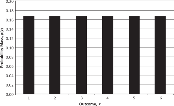
To illustrate these properties, let X be the outcome of tossing one standard (six-faced) die. Then the sample space for the random variable is simply the set of integers from 1 through 6, and the probability function is given by the frequency 1/6 for all values in the sample space, as shown in the histogram of Figure 2.1. This random variable possesses several special properties worth noting: Its sample space is discrete, consisting of a set of elements, x, that can be indexed by the positive integers (in this case, the numbers from 1 through 6); its sample space is finite, comprising only six elements; and its probability function, p(x), is uniform (i.e., constant) over all the elements in the sample space.
PMF of One Die Roll (i.e., Discrete Uniform Random Variable Defined on {1, 2, 3, 4, 5, 6})
As a matter of terminology, any random variable whose sample space is discrete is, quite naturally, said to be a discrete random variable. At first glance, one might suspect that all such random variables have finite sample spaces, but that is not true. Consider, for example, a different random variable X whose sample space is the infinite set of all positive integers, {1, 2, 3, … }, and whose probability function begins with a p(1) of 1/6, and then decreases by a factor of 5/6 each time x increases by one unit. This particular probability distribution, called the geometric distribution with parameter 1/6, is captured by the histogram in Figure 2.2 and is very similar to the age-at-death probability distribution presented in Figure 1.6.4
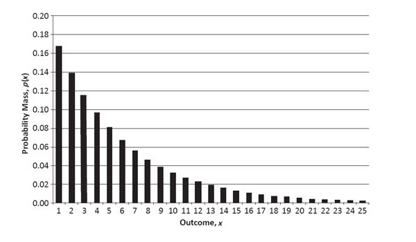
PMF of Geometric Random Variable with Parameter 1/6 (Defined on Positive Integers)
For the geometric random variable, the sample space is both discrete and infinite. Nevertheless, there is a price to pay for extending the sample space to the infinite set of positive integers: namely, having to use a more complicated probability function to make sure that the individual probabilities, p(x), add up to 1. In fact, to construct a random variable whose sample space is both discrete and infinite, one must give up any hope of having a uniform probability function. Another way of saying this is that it is impossible to select a positive integer at random in such a way that each integer is equally likely to be chosen.5
Although accepted with little thought by statisticians, this last observation is quite interesting, perhaps even profound. Essentially, what it means is that we, as “acquaintances” of the integers, can never be truly egalitarian in our associations; inevitably, we must favor an incredibly small subset in some finite neighborhood {1, 2,…, n}, where the magnitude of n—whether recorded in thousands, millions, or googols6—is dwarfed by an infinitely greater set of completely unfamiliar larger integers.
Paradoxically, despite the foregoing discussion, there does remain a way to construct a random variable that possesses both an infinite sample space and a uniform probability function. To accomplish this, however, one must relinquish the property of discreteness.
The Continuum
As noted above, a discrete sample space consists of a set of elements, x, that can be indexed by the positive integers. In other words, the total number of elements in such a set can be no larger than the total number of elements in the set of positive integers—that is, no larger than infinity. This seems like an easy condition to satisfy and, in fact, an impossible one to contradict. So how can a sample space not be discrete? To find such spaces, one first must find a number that is, in some sense, “larger” than infinity itself!
One approach to breaking through the “infinity barrier” might be to attempt to double the size of the set of positive integers by adding the equally large set of negative integers to it. More precisely, letting {1, 2, 3, … } be the set of positive integers and { …, -3, -2, -1} be the set of negative integers, one could consider the conjoined set, { …, -3, -2, -1, 1, 2, 3, … }. If N denotes the (infinite) number of elements in either {1, 2, 3, … } or { …, -3, -2, -1}, then the number of elements in { …, -3, -2, -1, 1, 2, 3, … } must be 2 X N. However, as will be seen, 2 X N is actually no larger than N.
To compare the sizes of two different infinite sets, one must attempt a one-to-one matching between their respective elements. If each element in one set can be associated with a unique element in a second set, without any elements being left over in either set, then the two sets are said to have the same cardinality (size). If, however, there are some elements left over in either of the two sets after the matching takes place, then the set with the extraneous elements is said to have a larger cardinality.
Now consider what happens if one attempts to match the elements of { …, -3, -2, -1, 1, 2, 3, … } with those of {1, 2, 3, … }. Suppose one writes the elements of the former set as {1, -1, 2, -2, 3, -3, … }, and then matches the first, third, fifth, etc. members of this list with the positive integers 1, 3, 5, etc. while matching the second, fourth, sixth, etc. members of the list with the positive integers 2, 4, 6, etc. A careful examination of this pairing reveals that it is indeed one-to-one, with no elements left over in either set. Consequently, the cardinalities of the two sets must be the same, and so 2XN equals N. More generally, if m is any finite positive integer, then m X N equals N. Rather remarkably, even multiplying N by itself a finite number of times does not increase its cardinality, and so neither the addition nor multiplication of Ns is sufficient to obtain a number larger than N.
The German logician Georg Cantor was the first to overcome the infinity barrier, and he did so by using exponentiation.7 Specifically, he was able to prove that the number m X m X … X m [N times], where m is any finite positive integer greater than 1, is larger than N. Interestingly, this new number, called C, denotes the cardinality of the set of real numbers in the interval from 0 to 1. Any set of this cardinality is called a continuum.
To see why the number of points in the interval [0,1) is given by C, first note that any real number between 0 and 1 can be represented as an infinite decimal expansion o.d1d2d3 …, where each of the digits d1, d2, d3, … equals one of the ten distinct digits 0, 1, 2,…, 9. Then, to count how many such expansions exist, simply observe that there are ten possible values for d1, ten possible values for d2, ten possible values for d3, etc. It immediately follows that the total number of expansions must be 10 X 10 X … X 10 [N times], which equals C (since m may be taken to equal 10).
Let us now consider how to select a number at random from the infinite set—or continuum—of real numbers in [0,1) in such a way that each real number has the same chance of being chosen. Intuitively, this could be accomplished by using an infinitely thin knife to slice the interval into two pieces, with each point in [0,1) equally likely to serve as the cutting point. But to express this idea formally, I need to introduce the concept of a continuous random variable—that is, a random variable whose sample space is a continuum.
Let Y denote a random variable whose sample space consists of all the real numbers in the interval [0,1). Since I now am dealing with a continuum, I cannot simply break up the sample space into a collection of discrete points, y, for which a probability function can be stated. Rather, I must partition it into a large number (n) of small intervals, each of equal length, 1/n. I then can write the probability for the ith interval—denoted by p(yi)—as f(yi) X (1/n), where f(yi) is the relative likelihood (frequency) with which Y takes on a value in that particular interval (compared with the other intervals of equal length).
If Y is a uniform random variable, then I know that f(yi) must equal some constant value, k, for each interval. Given that the sum of the probabilities p(yi) must equal 1, it follows that k equals 1 and thus p(yi) equals 1/n, as shown in the histogram of Figure 2.3.
Now consider what happens as n becomes infinitely large, so that each interval shrinks toward a single point in the [0,1) continuum. Clearly, this will cause the probabilities functions, p(yi), to shrink to 0, and so the probability associated with any given point in the continuum must be exactly o. Note, however, that at the same time the value of each probability decreases to o, the number of these probabilities increases to infinity (actually, to C). Thus, by the magic of the calculus, the “sum” of the probabilities can still equal 1.
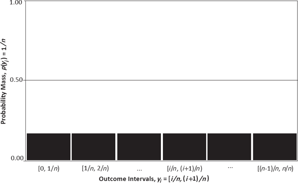
Forming a Continuous Uniform Random Variable (Defined on Interval [0, 1))
Here, then, is a bit of a puzzle: If I can “sum up” an infinite number of ο-valued probabilities in the continuum to obtain 1, then why am I unable to do the same thing with the positive integers? In other words, what prevents me from selecting an element from the set of positive integers with uniform probability simply by setting p(x) equal to 0 for each integer x, and then “adding up” all the 0s to get 1?
The resolution of this paradox rests on the fact that probabilities are defined quite differently for continuous and discrete sample spaces.8 In the former case, p(yi) equals f(yi) X (1/n), where f(yi) indicates a probability density spread out over the ith small interval (of length 1/n). In the latter case, p(x) denotes a probability mass associated with the individual point x. It thus follows that probabilities of ο can be assigned to all individual points in a continuous space while still preserving positive densities over various small intervals. Assigning probabilities of ο to all points x in a discrete space, however, leaves no masses to be accumulated.9
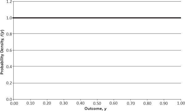
PDF of Continuous Uniform Random Variable (Defined on Interval [0, 1))
An important consequence of this difference is that when working with discrete random variables, one can use the probability function, p(x)—which henceforth will be called the probability mass function (PMF)—as plotted in Figures 2.1 and 2.2; however, when working with continuous random variables, one finds that p(y), which always equals 0, is useless, and so one must employ f(y)—the probability density function (PDF)—as plotted for the uniform distribution on [0,1) in Figure 2.4.
Just as the uniform random variable on [0,1) constitutes a continuous analogue of the discrete uniform random variable, the exponential random variable, whose PDF is presented in Figure 2.5 (for the parameter value 1/6), forms a continuous analogue of the geometric random variable. The exponential distribution shares with the geometric distribution the notable property of having a constant hazard rate (which naturally must be defined in continuous time, rather than discrete time). It also provides an example of a continuous distribution whose sample space goes from 0 to infinity and is therefore unbounded. Intriguingly, the cardinality of the unbounded continuum is exactly the same as the cardinality of any bounded continuum, that is, C. In other words, the real number line from 0 to infinity contains no greater number of points than does the interval from 0 to 1!
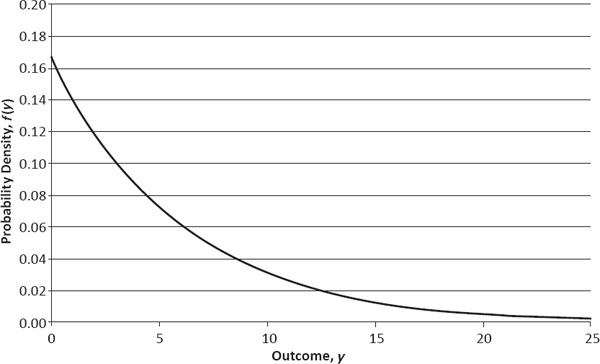
PDF of Exponential Random Variable with Parameter 1/6 (Defined on Positive Real Numbers)
Whence Probabilities?
As already mentioned, a random variable is intended to represent an unknown quantity. However, the use of a PMF, p(x), or PDF, f(y), clearly suggests that something is known about the variable. This observation raises an issue of deep philosophical (and practical) importance: How is information about the probabilities obtained?
To make the problem more concrete, let us return to a random variable discussed in Chapter 1—the ultimate age at death of a newborn baby—and focus on the histogram presented in Figure 1.1. Since a histogram is simply the plot of a discrete random variable’s PMF against the values in its sample space, it is easy to read from this figure the respective probabilities, pMale(x) or pFemale(x), that a newborn male or female baby will die at a given age, x. So where do these numbers come from?
The Frequency/Classical Paradigm
In the case of human mortality data, actuaries typically obtain the various probabilities of death by computing death rates from large samples of an actual human population. For example, pMale(45) = 0.0025 might result from observing that in a selected group of 10,000 U.S. males born in the same year, exactly 25 died at age 45. Essentially, this is the classical approach to estimating (approximating) probabilities, and it presupposes a frequency interpretation of the probabilities themselves.
By frequency interpretation, I mean that each probability p(x) is viewed as the long-run rate with which the outcome x—often called a “success” (even when a death is involved)—occurs among a sequence of repeated independent observations of the random variable. Thus, assuming that the life spans of individual males are unrelated to one another, the quantity pMale(45) denotes the overall proportion of males to die at age 45 among all males in the selected group.
Given the view of a probability as a long-run rate or proportion over a large, possibly infinite, population, it is natural to approximate the probability by considering a randomly chosen subset of the total population—called a sample—and using the observed ratio of the number of successes to the corresponding number of trials within that subset. This is the classical approach to estimation. Thus, the quantities pMale(x) or pFemale(x) in Figure 1.1 are not in fact the true probabilities associated with the age-at-death random variable, but only approximations of those probabilities and so are more properly written as  Male(x) or Female(x).10 From the law of large numbers (to be discussed further in Chapter 4), it is known that these approximations tend to become increasingly more accurate as the sizes of the associated random samples increase.
Life would be much simpler if the frequency interpretation of probability and the classical approach to estimation were appropriate for all random variables. However, as consequences of their very definitions, both paradigms run into obstacles in certain contexts. For the frequency interpretation, the principal difficulty is that many random variables are unique, rendering the concept of a sequence of repeated observations meaningless. Since the classical approach rests upon the frequency interpretation—otherwise, there is no basis for using a random sample to approximate p(x)—it follows that classical estimation also is inapplicable in the case of unique random variables. A further problem with the classical approach is that even if the frequency interpretation is in force, the law of large numbers has little effect when one is working with only a few repetitions in a sequence of observations.
In short, settings with unique random variables and/or few repetitions are problematic for the frequency/classical paradigm. Although such settings tend to arise at the extremes of human experience, they are still reasonably common in real life. Examples include: property perils associated with landmark buildings, historic monuments, and celebrated artwork; potential liabilities associated with large “one-time” sporting and music events; and perhaps most amusingly, accident/disability hazards associated with the specific talents of prominent entertainers and athletes (a dancer’s legs, a pianist’s hands, a tennis player’s elbow, etc.).
These types of risks are often termed “unique and unusual” in the insurance world, and special policies are written for them. Naturally, a major challenge for insurance companies is to obtain the probabilities p(x) associated with such random losses so that appropriate premiums can be charged. To see how this is accomplished, let us consider a hypothetical example.
Loaning Mona (The Subjective/Judgmental Paradigm)
Suppose that an insurance company underwriter has been asked by officials at the Philadelphia Museum of Art to provide property coverage for the Leonardo da Vinci masterpiece Mona Lisa while the painting is on a special thirty-day loan from the Louvre. Clearly, the subject work of art is unique, not just in the mundane sense that every fine painting is a unique expression of its creator, but more significantly, because it is the most widely recognizable—and perhaps the most valuable—Old Master painting in the world. Also, the exhibition is unique in that the painting has never traveled to Philadelphia previously and is unlikely to do so again in the foreseeable future.
For simplicity, the underwriter assumes that during its thirty-day visit, the Mona Lisa will be exposed to a limited number of perils—theft, fire, vandalism, terrorist attack, and natural disaster (including storm, flood, earthquake, volcano, etc.)—and that any loss would be total (i.e., there is no such thing as reparable partial damage). Although the painting is clearly priceless in the sense that it is truly irreplaceable, it does enjoy an assessable market value (i.e., the estimated amount that it would fetch at auction) that the underwriter assumes to be the equivalent of $1 billion.
Given these assumptions, the random variable of interest, X, has a sample space with just two points: x = 0 or x = 1 (in $billions). Analyzing things further, one can express p(1) as the sum
Probability of Theft + Probability of Fire + Probability
of Vandalism + Probability of Terrorist Attack+
Probability of Natural Disaster,
and p(0) as 1–p(1).
Now the question is: Given the uniqueness of the Mona Lisa’s sojourn in Philadelphia, what does it mean to speak of quantities such as probability of theft, probability of fire, etc.? Clearly, the frequency interpretation cannot apply, because there is no sense in which the thirty-day visit can be viewed as one observation from a sequence of repeated trials. Therefore, what is meant by a probability in this case is a purely cognitive metaphor or degree of belief—that is, something that the human brain apprehends as being equivalent to a frequency while not being a frequency per se. This is the subjective interpretation of probability.
Without the frequency interpretation, the underwriter naturally cannot use the classical approach to estimation. Just as the notion of probability itself is a cognitive metaphor under the subjective interpretation, so must be any estimation technique employed in conjunction with it. Consequently, the subjective interpretation restricts the underwriter to judgmental estimation methods. Such approaches come in various degrees of sophistication:
• Naïve Judgment. The simplest thing that an underwriter can do is to use his or her personal experience to estimate the value of a quantity such as probability of theft, without any formal method of aggregating this experience or rationalizing the final estimate. For example, when considering probability of theft, the underwriter may obtain the estimate 1/10,000 seemingly out of thin air, simply because this number appears to be appropriately small.
• Collective Judgment. Naturally, the highly personal nature of naïve judgment may make an underwriter feel somewhat insecure. After all, how would the underwriter explain his or her estimated probability if someone were to challenge it (which invariably would happen if the Mona Lisa were stolen)? To mitigate this problem, the most obvious thing to do is to seek safety in numbers by asking several additional professionals (e.g., fellow underwriters and/or actuaries) to provide independent estimates of probability of theft, and then to average these guesses to obtain a final estimate. For example, the underwriter might consult three professional colleagues and receive separate estimates of 1/1,000, 1/5,000, and 1/50,000. Averaging all these values with his or her own estimate of 1/10,000 then yields a final estimate of 33/100,000. Not only does this method provide the appearance of greater due diligence, but it also takes advantage of the frequency/classical paradigm (applied to judgmental estimates, rather than loss events) to reduce the variability of the final estimate.
• Educated Judgment. The principal problem with the above two approaches is that they do not employ any formal—or possibly even conscious—method of incorporating the estimators’ personal experiences into their estimates. To overcome this shortcoming, an underwriter may attempt to identify which particular items in his or her experience are most relevant to the estimation problem at hand, and then research, evaluate, and integrate these items in an intelligent way. For example, the underwriter may recall, following some reflection, that he or she once read an actuarial report summarizing art museum theft data. From an extensive Internet search, the underwriter then may locate the desired document and discover that it indicates an overall annual theft rate of 1/1,000—equivalent to a thirty-day probability of about 1/12,000—based upon several decades of loss experience from museums throughout the United States. Although this estimate is proffered under the frequency/classical paradigm, it is not directly applicable to the problem at hand because it is based upon: (1) old data; (2) paintings insured as part of a museum’s permanent collection; and (3) a cross-section of all paintings, rather than just the most valuable artwork. Nevertheless, the probability of 1/12,000 may serve as an upper bound on probability of theft if it is reasonable to assume that security measures: (1) have improved over time; (2) are better for visiting artwork than for permanent collections; and (3) are better for the most prominent artwork on display. While researching, the underwriter also may uncover the fact that the Mona Lisa itself was once stolen from the Louvre (in 1911). Dividing this one event by the roughly 200 years that the painting has been on display at the Louvre, he or she would obtain an annual theft rate of about 1/200—equivalent to a thirty-day probability of about 1/2,400. Again, although this estimate rests on the frequency/classical paradigm, it is not directly applicable to the current problem because it is based upon old data as well as the Mona Lisa’s history as part of the Louvre’s permanent collection. However, as before, the probability of 1/2,400 may serve as another upper bound on probability of theft. Given these analyses, the underwriter may conclude that 1/2,400 is a reasonably conservative (that is, high) estimate of the desired probability.
• Rational Judgment. Perhaps the most attractive type of judgmental estimate is one that can be supported by a logical or physical argument, without the need for individual guessing or empirical verification. For example, suppose that the underwriter has discussed matters with a game theorist who constructed a formal mathematical model of art theft based upon the opposing strategies of art thieves and museum security teams. Suppose further that under this game-theoretic model, the thirty-day probability of a painting’s being stolen is given by the expression √V /100,000,000, where √V denotes the square root of the painting’s value (in U.S. dollars).11 Plugging the Mona Lisa’s assessed value of $1 billion into this formula then yields an estimated probability of approximately 31,623/100,000,000.
Of course, a decision maker need not adhere exclusively to any one of the above estimation methods, and hybrid approaches—for example, averaging educated guesses with naïve guesses—are quite common.
To summarize, there are two principal pairings of probability interpretations and estimation methods: (1) the frequency/classical approach, often called frequentism, which requires both the possibility of repeated trials and a large number of actual repeated trials; and (2) the subjective/judgmental approach, often called Bayesianism,12 which works for unique trials and any number of repeated trials. Of these two, the latter approach is clearly more flexible.
Alternative Perspectives
The study of risk, like all mathematical disciplines, ultimately rests upon a foundation of intuition and metaphor.13 In formal expositions, this foundation is provided by a collection of assumptions called axioms (or postulates). Although mathematical purists might deny that such fundamental statements need be intuitively plausible—arguing that they are simply convenient starting points from which theory can be derived—any theory arising from a set of axioms without a strong metaphorical connection to basic human intuitions is difficult to peddle in the marketplace of ideas.
In introducing the various concepts of this chapter, I have focused on those ideas and methods that I believe appeal most strongly to human intuition; and that is the approach I will pursue throughout the remainder of the book. The price to be paid for such an emphasis is that many less-intuitive paradigms will be afforded scant attention or even completely ignored.
One significant mathematical theory possessing a nonintuitive foundation is possibility theory, a “fuzzy” alternative to traditional probability theory based upon the denial of Aristotle’s law of the excluded middle (LEM).14 A cornerstone of formal logic, the LEM states that “either a proposition is true, or its opposite is true—there is no third alternative.” Although few assumptions would seem more unassuming and self-evident than the LEM, a variety of interesting and provocative techniques have grown out of its negation.
Methods denying the LEM have been found to be particularly useful in contexts in which it is difficult to draw clear lines of demarcation between categories of entities, as in the detection of insurance fraud, where one cannot separate claims easily into two mutually exclusive and jointly exhaustive categories—“fraudulent” and “legitimate”—because of various intermediary cases: moral hazard, opportunistic fraud, litigiousness, etc.15 Nevertheless, these approaches have not gained great traction among scholars, at least partly because they negate the highly intuitive LEM.
Two decades ago, British statistician Dennis Lindley staked out the (somewhat extreme) anti-fuzzy position as follows:16
Probability is the only sensible description of uncertainty and is adequate for all problems involving uncertainty. All other methods are inadequate…. Anything that can be done with fuzzy logic, belief functions, upper and lower probabilities, or any other alternative to probability can better be done with probability.
Whether or not Lindley’s claim that “probability is the only sensible description of uncertainty” will be judged legitimate or fraudulent by history remains an open question. But as a purely philosophical matter, I would observe that a proposition that denies its opposite (i.e., is consistent with the LEM) seems more cogent than one admitting of self-contradiction.
ACT 1, SCENE 2
[A police interrogation room. Suspect sits at table; two police officers stand.]
GOOD COP: Hello, Ms. Cutter. I understand that you’ve waived your right to legal counsel; is that correct?
SUSPECT: Well, not really.
GOOD COP: Not really?
SUSPECT: No. You see, I’m an attorney myself, and so I can’t avoid having legal counsel present.
GOOD COP: Oh, well, that’s fine, of course. What I meant to say is, you’ve waived your right to additional legal counsel, is that correct?
SUSPECT: Yes, Officer; that is quite correct.
GOOD COP: Now, Ms. Cutter, I must be perfectly frank—the evidence against you is rather overwhelming. During the past year, the bodies of twelve separate murder victims have been found across the Commonwealth of Pennsylvania. In each case, the victim was killed in the same manner: While he or she slept, the killer sliced through the victim’s jugular vein—cleanly and deeply—with a crisp new $1,000 bill.
SUSPECT: A rather unusual weapon, don’t you think?
GOOD COP: Yes, it certainly is. And I think you’ll be interested to know that we found your fingerprints—yours and yours alone—on each of these “unusual weapons.” Can you explain that?
SUSPECT: No, I’m afraid I can’t. Not only can I not explain it, but I can’t understand it.
BAD COP: Look, lady, I don’t know what kind of word games you think you’re playing. What my partner is telling you in his polite, but somewhat roundabout way is that this is an open-and-shut case; we already have all the evidence needed to put you on death row. So if you want to do yourself a favor, then answer the questions; and maybe the judge will be in a better mood when he sentences you.
SUSPECT: I assure you it has been my intention all along to cooperate. I simply said that I don’t believe your partner’s assertion that no one else’s fingerprints were on the $1,000 bills. You see, when I picked them up at the bank, the bank teller must have handled at least some of them.
[Pause.]
BAD COP: Let me get this straight. You admit that the murder weapons belonged to you?
SUSPECT: Well, now it’s you who are playing word games. You call them “murder weapons,” but I’m afraid I can’t agree with that characterization.
GOOD COP: We’re talking about the crisp new $1,000 bills found at the twelve murder scenes. In all cases, they had blood on them—blood that matched the blood of the respective murder victims. And we have pathologists’ reports stating unequivocally that the bills were used to slit the victims’ throats.
SUSPECT: I agree. That is exactly how I killed them. But I insist that I did not “murder” them.
BAD COP: So what are you saying? That you killed a dozen people in their sleep, but it wasn’t murder? What was it: self-defense?
SUSPECT: No, it was an experiment.
BAD COP: What?
SUSPECT: It was an experiment—to test the “letter of the law.” Officers, do you happen to know how many citizens there are in the state of Pennsylvania?
GOOD COP: About twelve million, I believe.
SUSPECT: Yes, almost twelve and one-half million, in fact. And how many people did I kill?
GOOD COP: Well, we believe you killed twelve. That’s what our questions are about.
SUSPECT: Yes, I killed twelve; twelve out of twelve and one-half million. Do you know what proportion of the state population that is?
BAD COP: What does that matter?
GOOD COP: Twelve divided by twelve and one-half million gives something less than 1/1,000,000.
SUSPECT: Yes, less than 1/1,000,000.
BAD COP: Again, so what? We’re talking about murder here. Your batting average doesn’t matter.
SUSPECT: Oh, but it does, Officer. Do either of you know what the term negligible risk means?
BAD COP: I’ve had about enough of—
GOOD COP: Let her talk. Go on, what about negligible risk?
SUSPECT: You see, the government, at both the state and federal levels, considers a death rate of less than 1/1,000,000 to be a negligible risk. That is, anything—be it pesticides, exhaust fumes, or whatever—that kills fewer than 1/1,000,000th of the population is considered so unimportant as to be ignored.
GOOD COP: Well—I thought I had heard every excuse in the book; but that one is new to me.
SUSPECT: Yes, I do believe it’s a true innovation. So I take it you’ll be releasing me?