CHAPTER 3
Default Risk: Quantitative Methodologies
In the previous chapter we analyzed agency and internal ratings. We stressed that banks were increasingly trying to replicate the agencies’ process in order to rate their largest counterparts. It is, however, impossible to allocate an analyst to each of the numerous smaller exposures on a bank’s balance sheet. One needs statistical approaches for segregating “good borrowers” from “bad borrowers” in terms of their creditworthiness in an automated way. The techniques used for retail and SME loans are typically scoring models. For publicly listed corporates, it is also possible to rely on equity-based models of credit risk.
Credit scoring is often perceived as not being highly sophisticated. At first sight it seems that the banking industry considers that nothing significant has been discovered since Altman’s (1968) Z-score. One gathers information on a small set of key financial variables and inputs them in a simple model that separates the good firms from the bad firms. The reality is totally different: Credit scoring is a very little piece of the large data-mining jigsaw. Data mining—and in particular, statistical pattern recognition—is a flourishing research area. For example, Jain, Duin, and Mao (2000) perform a short survey including most significant and recent contributions in the area of statistical pattern recognition. They list more than 150 recent working papers and published articles. Since then, a lot of new fields, such as support vector machines, have been investigated more in depth. From a practical viewpoint, this means that most current statistical models applied to credit risk are lagging far behind state-of-the-art methodologies. As a consequence, we anticipate that banks will be catching up in the coming years with the integration of nonparametric techniques and machine learning methods.
Credit scoring models apply to any type of borrower. For the largest corporates (those with listed equity), structural models may be an appealing alternative. Structural models, also called Merton-type models, are becoming very widespread in the banking community. Two major reasons account for their popularity: They tend to convey early warning information, and they also reflect the idea of a marked-to-market assessment of the credit quality of obligors.
In this chapter we first discuss the merits and the shortcomings of structural models of credit risk. We then turn to the main types of credit scoring models and discuss at length the measures that may be used to assess the performance of a scoring model, either in absolute terms or relative to other models.
ASSESSING DEFAULT RISK THROUGH STRUCTURAL MODELS
Structural, or firm-value-based, models of credit risk describe the default process as the explicit outcome of the deterioration of the value of the firm. Corporate securities are seen as contingent claims (options) on the value of the issuing firm. Once a model for the value of the firm process has been assumed and the capital structure of the firm is known, it is possible to price equity and debt using option pricing formulas.
Conversely, it is possible to extract some information about the value of the firm from the price of the quoted equity. Once this is achieved, an equity-implied probability of default can be calculated, thereby replacing the probability of default of traditional scoring models.
Structural models have gained wide recognition among professionals and have become a market standard in the field of default risk. One of the great features of this class of models is their ability to provide a continuous marked-to-market assessment of the creditworthiness of listed firms. Unfortunately, the underlying assumptions necessary to obtain simple formulas for probabilities of default are sometimes heroic. In this section we present the classic Merton (1974) model and discuss its insights and limitations. We then provide a nonexhaustive list of the refinements brought to the Merton approach in the credit pricing field. We also discuss how these models have been applied by practitioners to assess probabilities of default and extract early warning information about troubled companies.
The Merton Model
In their original option pricing paper, Black and Scholes (1973) suggested that their methodology could be used to price corporate securities. Merton (1974) was the first to use their intuition and to apply it to corporate debt pricing. Many academic extensions have been proposed, and some commercial products use the same basic structure.
The Merton (1974) model is the first example of an application of contingent claims analysis to corporate security pricing. Using simplifying assumptions about the firm’s value dynamics and the capital structure of the firm, the author is able to give pricing formulas for corporate bonds and equities in the familiar Black and Scholes (1973) paradigm.
In the Merton model a firm with value V is assumed to be financed through equity (with value S) and pure discount bonds with value P and maturity T. The principal of the debt is K. At any  , the value of the firm is the sum of the values of its securities:
  . In the Merton model, it is assumed that bondholders cannot force the firm into bankruptcy before the maturity of the debt. At the maturity date T, the firm is considered solvent if its value is sufficient to repay the principal of the debt. Otherwise the firm defaults.
The value of the firm V is assumed to follow a geometric Brownian motion1 such that2  . Default occurs if the value of the firm is insufficient to repay the debt principal:
  . In that case bond-holders have priority over shareholders and seize the entire value of the firm VT. Otherwise (if
  ) bondholders receive what they are due: the principal K. Thus their payoff is P(T,T) = min(K,VT) = K − max(K−VT,0) (see Figure 3-1).
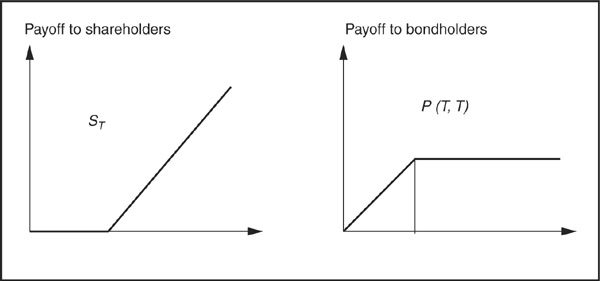
FIGURE 3-1
Payoff of Equity and Corporate Bond at Maturity T
Equity holders receive nothing if the firm defaults, but profit from all the upside when the firm is solvent; i.e., the entire value of the firm net of the repayment of the debt  falls in the hands of shareholders. The payoff to equity holders is therefore max
 (see Figure 3-1).
Readers familiar with options will recognize that the payoff to equity holders is similar to the payoff of a call on the value of the firm struck at K. Similarly, the payoff received by corporate bondholders can be seen as the payoff of a riskless bond minus a put on the value of the firm.
Merton (1974) makes the same assumptions as Black and Scholes (1973), and the call and the put can be priced using option prices derived in Black-Scholes. For example, the call (equity) is immediately obtained as

where

and where  denotes the cumulative normal distribution and r the riskless interest rate.
The Merton model brings a lot of insight into the relationship between the fundamental value of a firm and its securities. The original model, however, relies on very strong assumptions:
 The capital structure is simplistic: equity + one issue of zero-coupon debt.
 The value of the firm is assumed to be perfectly observable.
 The value of the firm follows a lognormal diffusion process. With this type of process, a sudden surprise (a jump), leading to an unexpected default, cannot be captured. Default has to be reached gradually, “not with a bang but with a whisper,” as Duffie and Lando (2001) put it.
 Default can only occur at the debt maturity.
 Riskless interest rates are constant through time and maturity.
 The model does not allow for debt renegotiation between equity and debt holders.
 There is no liquidity adjustment.
These stringent assumptions may explain why the simple version of the Merton model struggles in coping with empirical spreads observed on the market. Van Deventer and Imai (2002) test empirically the hypothesis of inverse co-movement of stock prices and credit spread prices, as predicted by the Merton model. Their sample comprises First Interstate Bancorp 2-year credit spread data and the associated stock price. The authors find that only 42 percent of changes in credit spread and equity prices are consistent with the directions (increases or decreases) predicted by the Merton model.
Practical difficulties also play a part in hampering the empirical relevance of the Merton model:
 The value of the firm is difficult to pin down because the marked-to-market value of debt is often unknown. In addition, all that relates to goodwill or to off-balance-sheet elements is difficult to measure accurately.
 The estimation of assets volatility is difficult due to the low frequency of observations.
A vast literature has contributed to extend the original Merton (1974) model and lift some of its most unrealistic assumptions. To cite a few, we can mention:
 Early bankruptcy and liquidation costs introduced by Black and Cox (1976)
 Coupon bonds, e.g., Geske (1977)
 Stochastic interest rates, e.g., Nielsen, Saa-Requejo, and Santa-Clara (1993) and Shimko, Tejima, and Van Deventer (1993)
 More realistic capital structures (senior, junior debt), e.g., Black and Cox (1976)
 Stochastic processes including jumps in the value of the firm, e.g., Zhou (1997)
 Strategic bargaining between shareholders and debt holders, e.g., Anderson and Sundaresan (1996)
 The effect of incomplete accounting information analyzed in Duffie and Lando (2001) (see Appendix 3A)
For a more detailed discussion on credit spreads and the Merton model, see Chapter 8.
KMV Credit Monitor Model and Related Approaches
Although the primary focus of Merton (1974) was on debt pricing, the firm-value-based approach has been scarcely applied for that purpose in practice. Its main success has been in default prediction.
KMV Credit Monitor applies the structural approach to extracting probabilities of default at a given horizon from equity prices. Equity prices are available for a large number of corporates. If the capital structure of these firms is known, then it is possible to extract market-implied probabilities of default from their equity price. The probability of default is called expected default frequency (EDF) by KMV.
There are two key difficulties in implementing the Merton-type approach for firms with realistic capital structure. The original Merton model only applies to firms financed by equity and one issue of zero-coupon debt: How should we calculate the strike price of the call (equity) and put (default component of the debt) when there are multiple issues of debt? The estimation of the firm value process is also difficult: How should we estimate the drift and volatility of the asset value process when this value is unobservable? KMV uses a rule of thumb to calculate the strike price of the default put, and it uses a proprietary undisclosed methodology to calculate the volatility.
KMV assumes that the capital structure of an issuer consists of long debt (i.e., with maturity longer than the chosen horizon) denoted LT (long term) and short debt (maturing before the chosen horizon) denoted ST (short term). The strike price default point is then calculated as a combination of short- and long-term debt: “We have found that the default point, the asset value at which the firm will default, generally lies somewhere between total liabilities and current, or short term liabilities” (Modeling Default Risk, 2002). The practical rule chosen could be the following:

The rule of thumb above is purely empirical and does not rest on any solid theoretical foundation. Therefore there is no guarantee that the same rule should apply to all countries and jurisdictions and all industries. In addition, little empirical evidence has been shown to provide information about the confidence level associated with this default point.3
In the Merton model, the probability of default4 is

where:
 = the cumulative Gaussian distribution
Vt = the value of the firm at t
X = the default threshold
σV = the asset volatility of the firm
μ = the expected return on assets
Example
Consider a firm with a market cap of $3 billion, an equity volatility of 40 percent, ST liabilities of $7 billion and LT of $6 billion. Thus  billion. Assume further that we have solved for A0 = $12.511 billion and
  percent. Finally
  percent, the firm does not pay dividends, and the credit horizon is 1 year. Then

And the “Merton” probability of default at a 1-year horizon is

The EDF takes a very similar form. It is determined by a distance to default:

Unlike Merton, KMV does not rely on the cumulative normal distribution  . Default probabilities calculated as N (–DD) would tend to be much too low due to the assumption of normality (too thin tails). KMV therefore calibrates its EDF to match historical default frequencies recorded on its databases. For example, if historically 2 firms out of 1000 with a DD of 3 have defaulted over a 1-year horizon, then firms with a DD of 3 will be assigned an EDF of 0.2 percent. Firms can therefore be put in “buckets” based on their DD. What buckets are used in the software is not transparent to the user. In the formula above, we use
  to denote the function mapping the DD to EDFs.
Figure 3-2 is a graph of the asset value process and the interpretation of EDF.
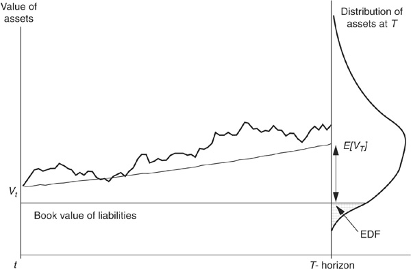
FIGURE 3-2
Relating Probability of Default and Distance to Default
Once the EDFs are calculated, it is possible to map them to a more familiar grid such as agency rating classes (see Table 3-1). This mapping, while commonly used by practitioners, is questionable for reasons explained in the previous chapter: EDFs are at-the-point-in-time measures of credit risk focused on default probability at the 1-year horizon. Ratings are through-the-cycle assessments of creditworthiness—they cannot, therefore, be reduced to a 1-year PD.
TABLE 3-1
EDFs and Corresponding Rating Class

Figure 3-3 is an empirical illustration of the structural approach to default prediction. It reports the 1-year PD and associated rating category for France Telecom stock, using a model similar to Merton or Credit Monitor. The effect of the collapse of the telecom bubble since March 2000 is clearly reflected in the probability of default of France Telecom.
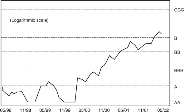
FIGURE 3-3
France Telecom 1-Year PD from Merton-Type Model
Uses and Abuses of Equity-Based Models for Default Prediction
Equity-based models can be useful as an early warning system for individual firms. Crosbie (1997) and Delianedis and Geske (2001) study the early warning power of structural models and show that these models can give early information about ratings migration and defaults.
There have undoubtedly been many examples of successes where structural models have been able to capture early warning signals from the equity markets. These examples, such as the WorldCom case, are heavily publicized by vendors of equity-based systems. What the vendors do not mention is that there are also many examples of false starts: A general fall in the equity markets will tend to be reflected in increases in all EDFs and many “downgrades” in internal ratings based on them, although the credit quality of some firms may be unaffected. False starts are costly, as they induce banks to sell their position in a temporary downturn and therefore at an unfavorable price.
Conversely, in a period of booming equity markets such as 1999, these models will tend to assign very low probabilities of default to almost all firms. In short, equity-based models are prone to overreaction due to market bubbles.
At the portfolio level this overreaction can be problematic. Economic capital linked to PDs calculated on the basis of equity-based models will tend to be very volatile. As a result, these models are unlikely to be favored by the top management of banks. The generalized usage of this kind of model by banks in a Basel II context would lead to a much increased volatility of regulatory capital (see Chapter 10) and to increased procyclicality in the financial sector. Equity-based models are indeed much more procyclical than through-the-cycle ratings because stock markets tend to perform well in growth periods and badly in recessions: Banks are therefore encouraged to lend more in good times and less when the economy needs it most.
To sum up, Merton-type models have become very popular among practitioners. Many banks have developed their own systems to extract early warning information from market variables. Many variants can be found that extract the volatility of the firm from either equity time series, implied volatilities in options markets, or even spreads. Vendors also supply their own interpretation of the structural approach. Equity-based models reflect the market’s view about the probability of default of specific issuers and can therefore provide valuable early warning signals. Unfortunately, they are no panacea, as they also reflect all the noise and bubbles that affect equity markets. Overall they can be seen as a useful complement to an analysis of a firm’s fundamentals.
CREDIT SCORING
The structural models presented above are based on equity information. They are therefore useful for listed companies but do not extend easily to smaller and private firms. For that purpose banks generally rely on credit scoring. In this section we provide a brief overview of the history of credit scoring. We proceed with an analysis of traditional scoring approaches and more recent developments and then discuss extensively the various performance measures that have been proposed to assess the quality of credit scoring models.
Scoring Methodologies
We begin by reviewing the history of credit scoring. We then turn our attention to an analysis of traditional scoring approaches, and finally we focus on more recent developments.
A Brief Retrospective on Credit Scoring
Quantitative models rely on mathematical and statistical techniques whose development leads the applications to credit scoring. Fitzpatrick (1932) initially established the dependence between the probability of default and individual characteristics for corporate credits. In the same period, Fisher (1936) introduced the concept of discriminant analysis between groups in a given population. Subsequently an NBER study by Durand (1941) used discriminant analysis techniques to segregate good and bad consumer loans. After the Second World War, large companies would use such techniques for marketing purposes.
A major breakthrough in the use of quantitative techniques occurred with the credit card business in the 1960s. Given the size of the population using such cards, automated lending decisions became a requirement. Credit scoring was fully recognized with the 1975 and 1976 Equal Opportunity Acts (implemented by the Federal Reserve Board’s Regulation B). These acts stated that any discrimination in the granting of credit was outlawed except if it was based on statistical assessments. Originally methods were based on what was called the “5 Cs”: character (reputation), capital (amount), capacity (earnings volatility), collateral, and condition (economic cycle).
In terms of methodology, the 1960s brought serious improvements. The use of credit scoring techniques was extended to other asset classes and in particular to the population of SMEs. Myers and Forgy (1963) compared regression and discriminant analysis in credit scoring applications, then Beaver (1967) came with pioneering work on bankruptcy prediction models, and Altman (1968) used multiple discriminant credit scoring analysis (MDA). This technique enables one to classify the quality of any firm, assigning a Z-score to it. Martin (1977), Ohlson (1980), and Wiginton (1980) were the first to apply logit analysis to the problem of bankruptcy prediction.
All these approaches focused both on the prediction of failure and on the classification of credit quality. This distinction is very important, as it is still not clear in the minds of many users of scores whether classification or prediction is the most important aspect to focus on. This will typically translate into difficulties when selecting criteria for performance measures.
Credit scoring has now become a widespread technique in banks. The Federal Reserve’s November 1996 Senior Loan Officer Opinion Survey of Bank Lending Practices showed that 97 percent of U.S. banks were using internal scoring models for credit card applications and 70 percent for small business lending. These figures have increased over the past 5 years, in particular with the Basel II focus on probabilities of default. In 1995 the largest U.S. provider of external models, Fair, Isaac and Company, introduced its first Small Business Credit Scoring model5 using data from 17 and then 25 banks. Today there are several providers of credit models and credit information services in the market.
The major appeal of scoring models is related to a competitive issue. They enable productivity growth by providing a credit assessment in a limited time frame with reduced costs. Allen (1995) reports that based on credit scoring, the traditional small-business loan approval process averages about 12 hours per loan, a process that took up to 2 weeks in the past.
Berger, Frame, and Miller (2002) review the impact of scoring systems on bank loans to the lower end of the SME business6 in the United States over the period 1995–1997. They show that the use of scoring systems within banks is positive in the sense that it tends to increase the appetite of banks for that type of risk and that it reduces adverse selection by enabling “marginal borrowers” with higher risk profiles to be financed more easily, but at an appropriate price. Interestingly, Berger, Frame, and Miller were unable to confirm the real benefit of scoring systems for larger loans (between $100,000 and $250,000), but their database is more limited over that range.
The most widespread current credit scoring technologies consist of four multivariate scoring models: the linear regression probability model, the logit model, the probit model, and the multiple discriminant analysis model. These models are fairly simple in terms of structure and will be reviewed in the next section together with newer, more advanced models.
Choosing the optimal model, based on an existing data set, remains a real challenge today. Galindo and Tamayo (2000) have defined five requisite qualities for the choice of an optimal scoring model:
1. Accuracy. Having low error rates arising from the assumptions in the model
2. Parsimony. Not using too large a number of explanatory variables
3. Nontriviality. Producing interesting results
4. Feasibility. Running in a reasonable amount of time and using realistic resources
5. Transparency and interpretability. Providing high-level insight into the data relationships and trends and understanding where the output of the model comes from
The Common Range of Credit Scoring Models
In this section we analyze the most popular models used in credit scoring. We also describe newer methodologies that are being introduced to credit scoring problems. We believe that some of these techniques will progressively be implemented in more sophisticated banks.
Figure 3-4 is an overview of the various classes of models we consider in this section. This classification is inspired by Jain, Duin, and Mao (2000).

FIGURE 3-4
Classification of Pattern Recognition Approaches
In statistical pattern recognition, it is common to find a distinction between supervised and unsupervised classification. The difference between the two approaches is that in the first case, we know according to which criteria we want to classify firms between groups. In the second case, in contrast, the model builder seeks to learn the groupings themselves from the model. In the section that follows, we only consider supervised classification.
The models listed in parts (I) and (II) of Figure 3-4 will be described later in the chapter, as part of the performance measure framework. The reason for this is that the underlying rules to which they correspond do matter when defining optimal classification or optimal prediction.
In this section we focus on four different approaches (with corresponding references in Figure 3-4):
 Fisher linear discriminant analysis (III)
 Logistic regression and probit (III)
 k-nearest neighbor classifier (IV)
 Support vector machine classifier (V)
These four approaches encompass the most widely used techniques in the credit scoring arena. Many other techniques exist, such as neural networks, tree induction methods, and genetic algorithms. These are treated in statistical pattern recognition books such as Webb (2002).
The first two types of classifiers we mention (discriminant and logit/probit) will often be used as front-end tools7 because they are easy to understand and to implement. Their main strength corresponds above all to classification accuracy and ease of use. The last two (nearest neighbor and support vector machines) are often seen as back-end tools, because they require longer computational time. Their value is based on high predictive performance standards.
Fisher (1936) Linear Discriminant Analysis The principal aim of discriminant analysis is to segregate and classify a heterogeneous population in homogeneous subsets. In order to obtain such results, various decision criteria are used to determine a relevant decision rule.
The idea is quite simple: We first select a number of classes C in which we want to segregate the data. In the case of a credit scoring model, there can be, for example, two classes: default and nondefault. Then, we look for the linear combination of explanatory variables which separates the two classes most.
Before we can get into the details of the models, we need to introduce some notations:
n is the number of data points to be separated—for example, the number of borrowers of a bank.
p is the number of variables available for each data point. In the case of credit scoring, the variables8 would be, for example, plain amounts like EBIT, total assets, liabilities, or ratios like gearing.
 is the vector of observations of the random variables
  .
.
C denotes the number of categories in which the data will be classified. In the case of a good loan–bad loan separation, there are only two categories:  .
.
μi denotes the mean of the variables in class i.
Σ is the between-class covariance matrix.
Let us now consider the Fisher approach to separate two classes ω1and ω2 such as “good borrowers and bad borrowers.” Fisher’s idea is to look for the linear combination of explanatory variables which leaves the maximum distance between the two classes.
His selection criterion can be written as maximizing

where w is the vector of weights that needs to be found. The numerator is the global covariance, and the denominator is the variance.
The maximum is obtained by differentiating F with respect to the vector of weights and setting the differential equal to zero:

The unique solution is

A pattern x (i.e., a borrower in the case of credit scoring) is then assigned to group ω1 if  and to group ω2 if
  .
.
Maximizing F does not, however, provide a rule to determine α, i.e., the cutoff point separating classes ω1 and ω2. In general, it has to be chosen by the user.
The most famous application of discriminant analysis to credit scoring is Altman’s (1968) Z-score. Explanatory variables used in this model include working capital/assets, retained earnings/assets, EBIT/assets, net worth/liabilities, and sales/assets.
Example
The comparison between the conditional probability of default P(D|L) and the a priori default probability PD enables us to qualify the riskiness of a company for which the score belongs to L. If  , then there is high risk; otherwise no. The more significant the difference, the higher the risk (Figure 3-5).

FIGURE 3-5
Separating Companies Using a Discriminant Ratio
Parametric Discrimination Assume that  , is the score function. Once α is chosen, Fisher’s rule provides a clear-cut segregation between ω1 and ω2. It does not provide probabilities of being in one class or another, conditional on observing realizations of the variables.
In most cases the choice will not be as simple as being either in class ω1 or in class ω2, and one would need probabilities of being in a given class. A very crude approach would be to apply a simple linear regression and say that  , this means that the probability of being in class ω2 (for example, default) conditional on observing realizations of the variables x (for example, financial ratios9), is simply equal to the score. This is not adequate, as the probability should be between 0 and 1, whereas the score is generally not bounded.
One way to get around this problem is to apply a transformation to the score in order to obtain a probability that lies in the interval [0,1].
Linear Logit10 and Probit
Let us first consider that the score has the following relationship with the probability:

Then it can be shown that

where β is a constant that reflects the relative proportion of firms in the two classes:

Equation (3-2) gives the conditional probability of the firm being in class ω2 (defaulting) conditional on a realization of its variables (financial ratios). The probability follows a logistic law, hence the name logit model. Other transformations are possible, such as using the normal distribution, leading to the normit model—more commonly known as the probit model. In both cases the estimation of the parameters is performed by maximum likelihood. The main difference between the two approaches is linked to the fact that the logistic distribution has thicker tails than the normal distribution (see Figure 3-6). However, this will not make a huge difference in practical applications as long as there are not too many extreme observations in the sample.
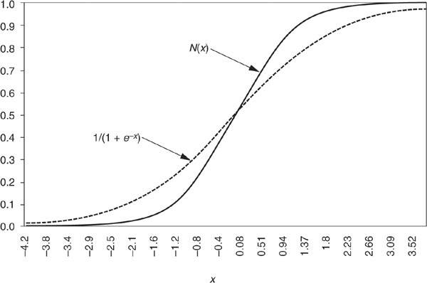
FIGURE 3-6
Logistic and Normal Cumulative Distribution Functions
The decision rule for classifying patterns (borrowers) remains as simple as in the linear discriminant case: Assign a borrower with observed financial ratios x to class ω1 if  ; otherwise assign it to ω2. The estimation of w is performed using maximum-likelihood techniques. The larger the training sample on which the weights are estimated, the closer it is from the unknown true value.
Engelmann, Hayden, and Tasche (2003) provide an empirical comparison of the logit model and Altman’s Z-score (discriminant analysis) on a large sample of SMEs. They show a very significant outperformance of the logit model in terms of rank ordering (the ROC coefficient11).
Example
In regard to the weights on factors using a logit model on a set of SME companies (Figure 3-7). These weights have been determined using a maximum-likelihood approach on a training sample.
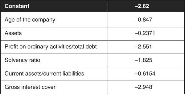
FIGURE 3-7
Example Parameters of a Logit Model
Nonlinear Logit
Linear logit models assume by definition a linear relationship between the score and the variables. More complex relationships such as nonmonotonicities are ignored factors. Let us take an anecdotal example of a variable that has been shown to exhibit a nonmonotonic relationship with the probability of financial distress in the SME market: the age of the manager.
When the manager of a small firm is very young, she is inexperienced and often not risk averse. Young age will therefore tend to be associated with a high riskiness of the firm. Then as the manager becomes more mature, she will have gained experience, may have a mortgage and a family and therefore be more prudent. However, as she approaches retirement, her potential successors may start fighting for power, or her heir, who has no notion of the business, may be about to take over. Therefore old age also tends to be associated with high risk. The relationship between age and riskiness is thus U-shaped and not monotonic. It cannot be described satisfactorily by a linear function.
Laitinen and Laitinen (2000) suggest applying a nonlinear transformation to the factors T(x) such that

where the data transformation could be the Box-Cox function:

where λi is a convexity parameter: If  , the transformation is concave; if
  , it becomes convex.12
Many other transformations are possible, including the quadratic logit model. It is an immediate extension of the linear logit model presented above. Instead of considering only the first-order terms, the quadratic logit model also includes second-order terms:

where β is a constant and δs and γs are the weights. It has the advantage of not only including the possibility of a nonlinear relationship between the score and each explanatory variable but also incorporating interactions between variables via the product xixj.
These models have more parameters and will therefore tend to provide a better fit and have more predictive power than simple linear models. They remain relatively simple to estimate on the data.
Nonparametric Discrimination: The k-Nearest Neighbor Approach13 The k-nearest neighbor (kNN) classifier is one of the easiest approaches to obtaining a nonparametric classification. In spite of (or thanks to) this simplicity, it has been widely used because it performs well when a Bayesian classifier14 is unknown. The entire training set is the classifier.
The kNN technique assesses the similarities between the input pattern x and a set of reference patterns from the training set. A pattern is classified to a class of the majority of its k-nearest neighbor in the training set. The classification is based on a basic idea expressed by Dasarathy (1991): “Judge a person by the company he keeps.”
Figure 3-8 is a simple graphical example of kNN classification. We want to classify good firms (those that won’t default) and bad firms (those that will) using two explanatory variables: return on assets (ROA) and leverage. Clearly, the higher the ROA and the lower the leverage, the less risky the firm. A set of good firms and bad firms has been identified in a training sample, and we want to classify a new firm. We choose  . Looking at the six nearest neighbors of the new firm (those within the circle), we can see that four of them are good firms and only two are bad firms. The new borrower will therefore be classified as good.
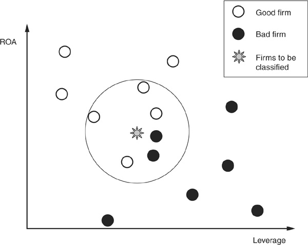
FIGURE 3-8
k-Nearest Neighbor Classification
The distance chosen to identify the nearest neighbors is crucial for the results. Several options have been proposed, and the choice of distance metric has been one of the avenues of research taken to improve the performance of this methodology. The most frequently used is the Euclidean distance. Assume that we have values for p variables (in the example above,  , corresponding to leverage and ROA) of a given firm we want to classify: x1, x2,…, xp and that the corresponding values for a firm in the training set are y1, y2,…, yp. The Euclidian distance between the two firms is

One of the main drawbacks of the kNN technique is that it can prove time consuming when the sample size becomes large. Indeed if we consider a training set of n patterns,  distances should be calculated in order to determine the nearest neighbors (the number of variables p may be large as well). For a reasonable data set of SMEs of 10,000 firms, it involves the calculation of nearly 50 million distances. Manipulations of the patterns in the training set to reduce the time and space complexity have therefore been introduced by several authors.
The choice of k (the number of neighbors to consider) is also important. For example, if we had chosen  in the example above, we would have assigned the new borrower to the class of bad firms. In case k is too small, the classification may be unstable. Conversely, if it is really too large, some valuable information may be lost. Enas and Choi (1986) give a rule of
  , but there is no generally accepted best k.
Hand and Henley (1997) discuss the implementation of a kNN credit rating system with particular emphasis on the choice of distance metrics.
Support Vector Machines15 Support vector machines16 (SVMs) have been introduced by Cortes and Vapnik (1995). They have received a lot of interest because of their good performance and their parsimony in terms of parameters to specify. The main idea is to separate the various classes of data using a “best” hyperplane.
We first examine a linear support vector machine (LSVM). Assume that, as above, we have two types of borrowers (good and bad) and that we want to classify them according to two variables (ROA and leverage). If the data are linearly separable (i.e., if one can “draw a straight line” to separate good firms and bad firms), there are often many ways to perform this segregation. In Figure 3-9a we draw two lines17 A and B that separate the data.
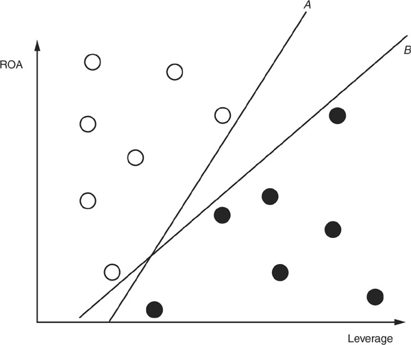
FIGURE 3-9a
Two Arbitrary Separations of the Data
LSVM provides a rule to select among all possible separating hyperplanes: The best separating hyperplane (BSH) is the hyperplane for which the distance to two parallel hyperplanes on each side is the largest. Figure 3-9b shows the BSH that separates the data optimally. Two parallel hyperplanes with the same distance to the BSH are tangent to some observations in the sample. These points are called support vectors (SV on the graph).
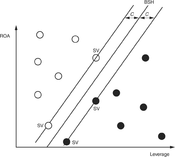
FIGURE 3-9b
Best Separating Hyperplane
The Case Where Data Are Linearly Separable
Points x on the best separating hyperplane satisfy the equation  . If we consider a set of training observations xi, where i ∈ {1,…,n}, an observation xi will be assigned to class ω1 according to the rule
  and to class ω2 according to the rule
  .
.
The rule can be expressed synthetically as  for all i, where
  if
if  and −1 otherwise.
The BSH does not provide the tightest separation rule. This is provided by the two hyperplanes that are parallel to the BSH and tangent to the data.
One can thus use a stricter rule:  , where c is the distance from the BSH to the tangent hyperplanes (called canonical hyper-planes).
Parameters of the hyperplanes are found by minimizing18 ||w||, subject to  . This is a standard mathematical problem.
The Case Where the Data Are Not Linearly Separable
The case considered above was simple, as we could find a straight line that would separate good firms from bad firms. In most practical cases, such straightforward separation will not be possible. In Figure 3.10 we have added only one observation, and the data set is no longer separable by a straight line.
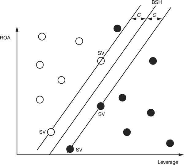
FIGURE 3-10
Nonlinearly Separable Data
We can still use linear support vector machines but must modify the constraints slightly. Instead of the strict rule wTxi + w0 > 0 that lead to being assigned to ω1, we use  , where Fi is a positive parameter that measures the degree of fuzziness or slackness of the rule.
Similarly, the slack rule will classify a firm in category ω2 if  .
.
A firm will then be assigned to the wrong category by the LSVM if  . The optimization program should include a cost function that penalizes the misclassified observations. Given that misclassification implied large values of Fi, we can adopt a simple rule such as, for example, to make the cost proportional to the sum of adjustments
  .
.
Nonlinear Support Vector Machine
Another way to deal with nonlinearly separable data is to use a nonlinear classifier h(x). The decision rule is similar but substitutes h(x) for x. Thus we obtain  for all i. This defines now the best separating surface.
The term h(xi)Th(xj) arises in the determination of the optimal parameter vector w. This term can be replaced by a kernel K(xi,xj) function.
Some popular choices for kernels are the Gaussian kernel:  and the polynomial kernel of order
  . For most kernels it is generally possible to find values for the kernel parameter for which the classes are separable, but there is a risk of overfitting the training data.
Figure 3-11 shows an example of how a nonlinear classifier can separate the data.
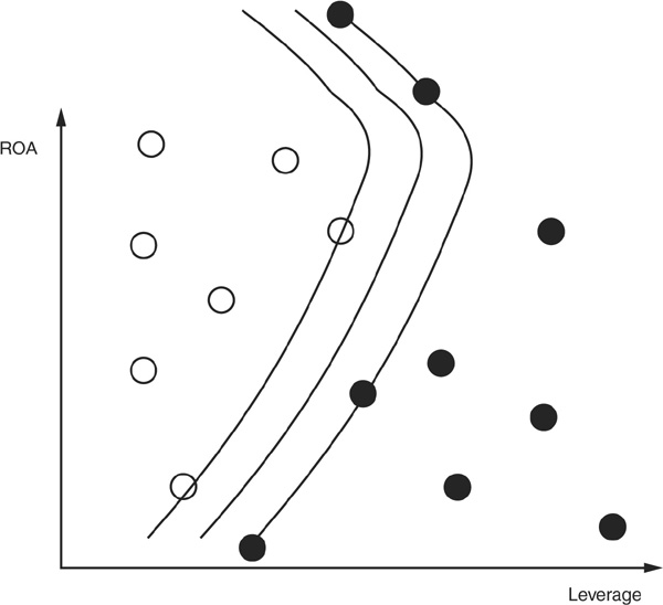
FIGURE 3-11
Nonlinear Kernel Support Vector Machine
Practical Implementations
Support vector machines are not only theoretically interesting; they are really applied by practitioners to credit data. For example, Standard & Poor’s CreditModel uses a fast class of SVMs called proximal support vector machines to obtain rating estimates for nonrated companies (see Friedman, 2002).
Model Performance Measures
The objective of this section is to introduce the various performance measures used to assess scoring models. A more detailed treatment of performance measurement can be found, for instance, in Webb (2002). This section follows some of its structure.
Performance measurement is of critical importance in many fields such as computer sciences, medical diagnosis, shape, and voice and face recognition. In credit analysis the stability of a bank may be at stake if the bank relies on a flawed credit model that persistently underestimates the risk of the bank’s counterparts.
The architecture of this section is organized according to Figure 3-12. We first describe performance measures that are widespread in statistical pattern recognition (classification tools). Second we review prediction tools that are particularly important for credit scoring. Then, before segregating the two approaches, we build on a common platform related to decision rules. In particular, we put emphasis on the description of a Bayesian framework, as it is the most common language for parametric and nonparametric modeling.
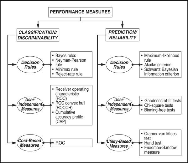
FIGURE 3-12
Classification of Performance Measures
Definition of Decision Rules
Here we introduce decision methodologies used to classify patterns. The space (the set of all possible combinations of variables) is divided into decision regions separated by decision boundaries. We first examine cases where class-conditional distributions and a priori distributions are identified.
If x is a vector that corresponds to a set of measurements obtained through observation and C is the number of different classes, then C is partitioning the space Ω in regions Ωi for  . If an observed measurement x is in Ωi, then it is said to belong to class ωi. The probability of each class occurring is known: p(ω1),…, p(ωC).
In credit terms, x would be the observed variables for a given firm (leverage, return on assets, profit and loss, and so on).
The “Minimum-Error” Decision Rule If we want to classify a firm with no prior information except the probability of a firm being in a given risk class ωk, we would assign it to the most probable class, i.e., class j defined as  .
.
Thus if the only information available is that there are two-thirds of good firms and one-third of bad firms, any new firm will be classified as good because it maximizes the unconditional (or a priori) probability.
If we have some data x about the explanatory variables, then the decision rule to assign x to class Ωj (and thereby the firm to ωj) is given by

p(ωj|x) is the conditional probability of being in class ωj, knowing x, also called a posteriori probability.
Using Bayes’ theorem, we can express the a posteriori p(ωj|x) with a priori probabilities p(ωj) and the class-conditional density functions p(x|ωj):

This can also be read as

The conditional decision rule can then be rewritten as

It is called Bayes’ rule for minimum error.
And the Bayes’ error is defined as

Regarding the choice between two classes a and b (such as between good borrowers and bad borrowers), the decision rule boils down to allocating the firm to class ωa if

and to class ωb otherwise. The rule is illustrated in Figure 3-13.

FIGURE 3-13
Bayes’ “Minimum-Error” Decision Rule
It can also be expressed as a likelihood ratio: x assigned the firm to class ωa if

and to ωb otherwise. p(ωb)/p(ωa) is the threshold.
The “Minimum-Risk” Decision Rule Other decision rules exist, such as minimum risk. The minimum-error rule consisted in selecting the class for which a posteriori  was the greatest.
A different rule can be chosen which minimizes the expected loss, i.e., the risk of misclassification. The costs of misclassification often have to be considered precisely. For instance, it can be more damaging to the bank to lend to a company that is falsely considered to be sound than to wrongly avoid lending to a sound company.
In order to reflect misclassification, a loss matrix C is defined whose elements cab are the cost of assigning a pattern x to ωb instead of ωa. The matrix will have to be defined by the user of the model according to the user’s own utility function. This task is often difficult to achieve because these costs are highly subjective.
Bayes’ expected loss or risk is then defined as

The Neyman-Pearson Decision Rule This classification rule applies to two-class problems, such as good and bad firms. With two classes, four types of events can occur, including two possible misclassification errors (EI and EII):
 The firm is bad and is classified as bad: right detection (1 − EI).
 The firm is bad and is classified as good: wrong detection of default EI
 The firm is good and is classified as good: right detection
  .
.
 The firm is good and is classified as bad: false alarm E II.
More formally, the two types of misclassification errors are
Type I error
 corresponding to the false nondefaulting companies
Type II error
 corresponding to the false defaulting companies
Being a false nondefaulting company is more dangerous than being a false defaulting company, because a loan will be granted to the former and not to the latter. A Type I error damages the wealth of the bank, given its utility function, whereas a Type II error is only a false alarm.
The Neyman-Pearson rule minimizes EI, with EII remaining constant. The solution is the minimum of

where μ is a Lagrange multiplier and  is the specified false alarm rate chosen by the user.
The rule will be to allocate the firm to region Ω1 if

and to Ω2 otherwise. The threshold μ is implied by the choice of  .
.
The Minimax Decision Rule The “minimax” concept refers to the objective of a maximum error or a maximum risk that is targeted to be minimum. To minimize the maximum error in a two-class environment, the minimax procedure consists of choosing the partitions Ω1 and Ω2 and minimizing:

The minimum is obtained when

That is, the regions Ω1 and Ω2 are chosen so that the probabilities of the two types of error are the same.
Performance Measures: Targeting Classification Accuracy
Now that we have surveyed the various decisions rules, we turn next to the subject of the different tools available, either for classification performance measures or for prediction performance measures. Appendix 3C reports practical issues regarding the assessment of credit scoring models.
Measuring Classification: The ROC Approach The ROC receiver operating characteristic measure and the Gini coefficient, described later, are probably the most commonly used approaches to measuring credit scoring performance.19 Figure 3-14 illustrates how to calculate the ROC coefficient. We assume that we have the output of a scoring model calibrated on a population with D defaults out of N firms.
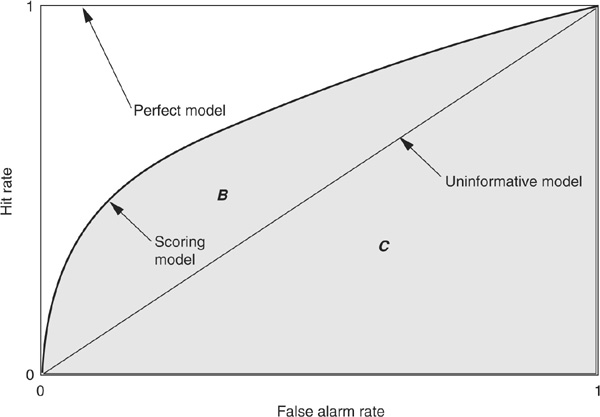
FIGURE 3-14
The ROC Curve
A score si and a probability of default pi are assigned to each firm  and the analyst chooses a cutoff level T such that the firm is considered bad if
  and good if
  .
.
For each firm, four cases are possible:
1. It defaults, and the model had classified it as bad (appropriate classification).
2. It defaults, and the model had classified it as good (Type I error).
3. It does not default, and the model had classified it as bad (Type II error, false alarm).
4. It does not default, and the model had classified it as good (appropriate classification).
We use as CT and FT to denote, respectively, the number of firms correctly and wrongly classified as bad (note that they depend on the cutoff level T). Then the hit rate H and false alarm rate F are:

The ROC curve is a plot of HT against FT. The steeper the ROC curve, the better, as it implies that there are few false alarms compared with correctly detected bad firms. On Figure 3-14 the perfect model is a vertical line going from (0,0) to (0,1) and then a vertical line linking (0,1) to (1,1). An uninformative model would on average have as many false alarms as correct detections and would result in a diagonal (0,0) to (1,1) ROC curve. Credit scoring models will produce intermediate ROC curves.
The ROC curve can also be seen as a trade-off between Type I (EI) and Type II (EII) errors. HT indeed corresponds to 1 − EI and EII to FT.
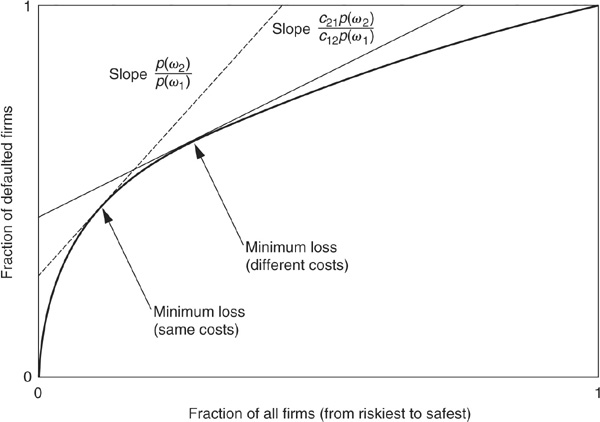
The ROC curve is also related to the minimum loss or minimum cost as defined above (see Figure 3-15). One starts by defining iso-loss lines whose slope is p(ω2)/p(ω1), the ratio of ex ante probabilities. By definition, any point on a given line corresponds to the same loss. The minimum loss point will be at the tangency between the ROC curve and the lowest iso-loss line.
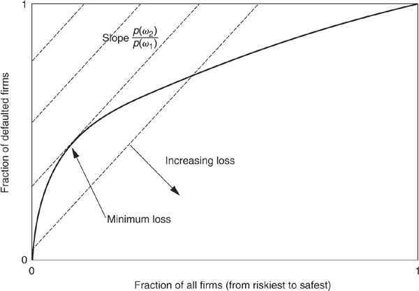
FIGURE 3-15
Finding the Minimum-Loss Point
The area below the ROC curve (either B or B + C) is widely used as a measure of performance of a scoring model. The ROC measure, however, suffers from several pitfalls. First, ROC is focused on rank ordering and thus only deals with relative classification. In credit terms, as long as the model produces a correct ranking of firms in terms of probabilities of default, it will have a good ROC coefficient, irrespective of whether all firms are assigned much lower (or higher) probabilities than their “true” values. Therefore one may have a model that underestimates risk substantially but still has a satisfactory ROC coefficient.
Second, ROC is an acceptable measure as long as class distribution is not skewed. This is the case with credit, where the nondefaulting population is much larger than the defaulting one. ROC curves may not be the most adequate measure under such circumstances.
In order to tackle the latter criticism, it is possible to include differing costs for Type I and Type II errors. Appendix 3D shows why it may be useful and how it affects the minimum-cost point.
Measuring Classification: The Gini/CAP Approach
Another commonly used measure of classification performance is the Gini curve or cumulative accuracy profile (CAP). This curve assesses the consistency of the predictions of a scoring model (in terms of the ranking of firms by order of default probability) to the ranking of observed defaults. Firms are first sorted in descending order of default probability as produced by the scoring model (the horizontal axis of Figure 3-16). The vertical axis displays the fraction of firms that have actually defaulted.

FIGURE 3-16
The CAP Curve
A perfect model would have assigned the D highest default probabilities to the D firms that have actually defaulted out of a sample of N. The perfect model would therefore be a straight line from the point (0,0) to point (D/N,1) and then a horizontal line from (D/N,1) to (1,1). Conversely, an uninformative model would randomly assign the probabilities of defaults to high-risk and low-risk firms. The resulting CAP curve is the diagonal from (0,0) to (1,1).
Any real scoring model will have a CAP curve somewhere in between. The Gini ratio (or accuracy ratio), which measures the performance of the scoring model for rank ordering, is defined as  , where E and F are the areas depicted in Figure 3-16. This ratio lies between 0 and 1; the higher this ratio, the better the performance of the model.
The CAP approach provides a rank-ordering performance measure of a model and is highly dependent on the sample on which the model is calibrated. For example, any model that is calibrated on a sample with no observed default and that predicts zero default will have a 100 percent Gini coefficient. However, this result will not be very informative about the true performance of the underlying models. For instance, the same model can exhibit an accuracy ratio under 50 percent or close to 80 percent, according to the characteristic of the underlying sample. Comparing different models on the basis of their accuracy ratio, calculated with different samples, is therefore totally nonsensical.
When the costs of misclassification are the same for Type I and Type II errors (corresponding to the minimum-error Bayesian rule), the summary statistics of the ROC and the CAP are directly related: If  on Figure 3-14) is the value of the area under the ROC curve and G is the Gini coefficient or accuracy ratio calculated on the CAP curve,20 then
  .
.
In this case the ROC curves and CAP curves convey exactly the same information. When a specific structure of costs of misclassification is introduced in the calculation of ROC, the link between the two curves is lost. ROC can probably be considered as more general than CAP because it allows for differing costs to be selected by the user.
Overall:
 The CAP curve provides valuable information if the user considers that misclassification costs are equal and provided the size of the defaulting subsample is somehow comparable with the non-defaulting one.21 If this is not the case, then another type of measure should complement the comparison of the performance of different models.
 Since bankers and investors are usually risk averse and would tend to avoid Type I errors more than Type II errors, CAP curves or Gini coefficients are not best suited to assess the performance of credit scoring models.
 The ROC measure is broader than the CAP measure because it enables the users of the model to incorporate misclassification costs or their utility function. If the objective is to assess the ability of the model to classify firms, then ROC, and in particular ROCCH22 is an attractive measure.
 A significant weakness of both the ROC and CAP approaches is that they are limited to rank ordering. This is a weak measure of performance in the area of credit where not only the relative riskiness but also the level of risk is crucial.
Performance Measures: Targeting Prediction Reliability
Until now we have discussed the ability to split a sample into subgroups such as good and bad borrowers. The focus was on the ability to discriminate between classes of firms, but not on the precise assessment of the probability of default. This is what prediction measurement is about: measuring how well the posterior probability of group membership is estimated by the chosen rule. Prediction reliability is a particularly important requirement in the credit universe, because a price (interest rate) may be associated with the output of a credit scoring model. If the bank’s credit scoring model underestimates risk systematically, it will charge too low interest rates and will thus, on average, make a loss.
The Maximum-Likelihood Decision Rule Geometric mean probability (GMP) is a measure similar to maximum likelihood that is easy to estimate. It is defined as

Given a model tested on a sample of N observations, the first term of the GMP focuses on truly defaulting companies i (where yi = 1), for which a probability of default p(xi) is assigned by the model. The second term of the GMP targets truly nondefaulting companies (where  ), for which a probability of default p(xi) is assigned by the model.
When comparing two different models on the same data set, the model with a higher GMP will be said to perform better than the other one. An ideal model would assign  percent to all defaulting companies and
  percent to all nondefaulting companies. Therefore GMP would be 100 percent.
From an economic standpoint, likelihood maximization can be seen as a measure of wealth maximization for a user of the scoring model. However, the underlying assumption is that the user of the model does not consider asymmetric payoffs. For the user, this means that all types of errors (EI, EII) have the same weight and impact on his wealth. Therefore likelihood measures can appear insufficient in the area of financial scoring where asymmetric payoffs matter.
What is interesting about likelihood is that it is primarily a simple aggregated measure of performance, whereas more complex well-established measures such as CAP and Gini focus more on misclassification and rank ordering.
There exist several additional criteria, based on likelihood, devised to compare different models. They tend to consider both likelihood and the number of parameters required to fit the model. The ultimate objective is to include what is called the “minimum description length” principle, which advantages the model having the shortest or more succinct computational description.
There are among others:
The Akaike (1974) information criterion (AIC):

The Schwartz (1978) Bayesian information criterion (BIC):
 , where k is the number of parameters, N the size of the sample, and
  the k-dimensional vector of parameter estimates. L(.) is the likelihood function.
The best model is supposed to minimize the selected criterion. Both BIC and AIC penalize models with many parameters and thereby reduce overfitting.
Some other tests exist such as Hand’s criterion.23
Measuring Prediction: Goodness-of-Fit Tests24 As with likelihood decision rules, the goodness-of-fit tests are devised to measure the deviation of a random sample from a given probability distribution function. In the following sections, the tests reviewed will be either distribution-free or adaptable to any type of distribution. We split between two types of tests, those that are applied to binned data and those that are applied to bins-free samples.
An Example of a Test Dependent on Binning: The Chi-Square Test
The purpose of the chi-square test is to analyze how close a sample drawn from an unknown distribution is to a known distribution. The chi-square test measures a normalized distance.
Assume that we have a large sample of N events that are distributed in K classes, according to a multinomial distribution with probabilities pi. Using Ni to denote the number of observations in class  (e.g., rating classes), we obtain

which follows asymptotically a χ2 distribution with  degrees of freedom.25
The probability α of a Type I error is related to the chi-square distribution by  It defines a level
  that determines the rejection of the null hypothesis
  (i.e., the hypothesis according to which the data sample follows the identified probability distribution function) is rejected at the α confidence level if
  .
.
An Example of the Use of a Chi-Square Test to Define Whether an Internal Scoring Model of a Bank Is Performing Well in Comparison with Expected Default
Let us consider a scoring system with 10,000 scores classified in 10 rating classes, 1 being the best class and 10 being the worst. Suppose 200 companies have actually defaulted. The null hypothesis is that the internal ratings classify in a satisfactory way, compared with the expected default rate per rating category.
The null hypothesis is H0: The model appropriately replicates the expected default rate.
We have the following observations:

The chi-square statistic is 41.6. The 95th percentile for a chi-square distribution with  degrees of freedom is 16.9. As the latter is significantly inferior to the statistic, it means that the hypothesis of the scoring system replicating the expected default rate satisfactorily should be rejected.
This test is easy to implement. It shows, however, some limitations:
 It depends highly on the choice of classes (binning).
 It assumes independent classes.
 It is accurate only when there is a reasonable trade-off between the number of events and the number of classes.
 It considers all deviations with the same weight.
An Example of Binning-Free Tests: The Kolmogorov-Smirnov Test
The test above relied on a specific bucketing (binning) of firms in risk classes. A way to avoid the impact of binning is to compare the empirical with the theoretical distribution.
The empirical distribution on a data sample with N observations is constructed as follows. We first rank the observations Xi in ascending order so that  . An empirical step distribution function is then built:

which is the fraction of observations below x.
Binning-free tests compare this empirical cumulative distribution with a theoretical distribution F(x) such as the normal distribution. The null hypothesis of the test is that the two distributions are identical.
The observed distance between the theoretical and empirical distribution is  .
.
The Kolmogorov difference is the maximum absolute difference:

The Kolmogorov-Smirnov test is based on the Kolmogorov difference. The null hypothesis [FN(x) corresponds to F(x)] is rejected if the Kolmogorov distance is sufficiently large:  is the cutoff value that depends on the confidence level α chosen for the test.
Measuring Prediction: Considering the Utility Function of the Model User
Over the past years, some financial institutions have tried to consider credit scoring, more with the perspective of maximizing profit than minimizing risk. The term used to refer to this approach is “profit scoring.” Profit scoring can, however, prove a difficult task to achieve, for several reasons:
 Solving data warehousing problems in order to take into account all elements that make up the profit
 Deciding between transaction profit and customer profit
 Selecting an appropriate time horizon to consider profit
 Including economic variables in profit scoring
 Understanding better current and future customers’ behavior (attrition rate, expected profit on future operations, etc.)
The choice among default scoring, risk scoring, and profit scoring will often be very specific to each financial institution. It reflects different governance profiles, i.e., different utility functions. In this section we will focus on utility maximization. We could have chosen to put more emphasis on cost minimization, but the maximization of a utility function under a cost constraint is equivalent to minimizing costs under a utility constraint.
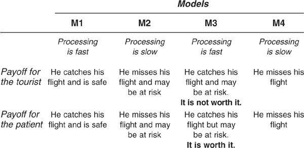
From a practical standpoint, we know that spelling out the costs of misclassification is difficult. We have intuitively observed that these costs were specific to the user of the models: the investor, the banker, or, as in the example of Appendix 3D, the tourist and the patient.
In order to make the measure of performance user-specific, we introduce a utility function and describe the approach by Friedman and Sandow (2002). Their approach can be seen as an extension of the model selection with cost functions presented in Appendix 3D. The main difference is that instead of assigning costs (or payoffs) to misclassified firms (Type I and Type II errors), they assign a payoff to every outcome based on the utility function26 of the model user. For simplicity, we focus on the case of discrete payoffs, but their measure also works in the continuous case.
Assume that an investor invests his wealth on N assets, with by denoting the proportion of wealth invested in asset  . Naturally

Each asset will return a payoff of Oy.27 The true probability of each payoff to be received by the investor is denoted as py. It is unknown but can be estimated by the empirical probability  . The investor’s view of the true probability (i.e., the probability derived from his model) is qy.
The true and estimated maximum expected utilities the investor will derive from his investment are, respectively,28

and

where b* denotes the optimal investment weights corresponding to the allocation rule that maximizes the utility of the investor. This allocation is based on the output (q) of the model.
Now consider two models (i.e., two sets of probabilities) q1 and q2. The relative expected utility can be calculated as

Then the selection rule is that  , which implies that model 2 outperforms model 1.
The preferred class of utility function considered in Friedman and Sandow (2002) is the logarithmic family:

where W corresponds to the wealth of the investor.
The three parameters α, γ, and β allow for a lot of flexibility in the shape of the function. This class of utility function has the added advantage that it makes the model performance measure independent from the payoff structure.29
This approach is not limited to the logarithmic class of utility functions, but this class has several nice properties:
 It makes the relative performance measure above independent of the odds ratio.
 The model classification corresponds to the intuitive maximization of likelihood.
 It approximates the results obtained under other popular utility functions—very well in many cases.
 The classification rule takes an economic interpretation: maximization of the rate of growth in wealth.
Measuring Prediction: Pitfalls about Model Calibration and Reliability
We have shown in the previous section that the performance of a model is not only linked with its classification ability, but also with its predictive power. This is particularly important for banks that trade risk for return and need a reliable measure of performance for each of their obligors.
Regarding the performance of scoring systems, rank-ordering performance is not sufficient, and the calibration30 of a model can be unreliable, although its ability to discriminate may be satisfactory. We now review some common pitfalls of credit scoring systems:
 Scoring models frequently rely on parametric assumptions regarding the shape of the distribution of PDs, scores, and ratings in the firms’ sample. The models are designed to produce score distributions that are roughly bell-shaped (like a normal distribution) or at least “unimodal.” If the true data distribution is indeed unimodal, then calibrating the mean and the variance may provide a satisfactory fit to the data. Figure 3-17a shows the result of the calibration of a scoring model around a mean on the S&P rated universe. The scoring model classifies firms in 18 risk classes and correctly calibrates the mean probability of default. The parametric assumption about the data distribution, however, strongly biases the results since Standard & Poor’s universe rating distribution appears to have two peaks: one around the A grade and one around the B+ grade (see Figure 3-17b).

FIGURE 3-17a
Scoring Model Distribution
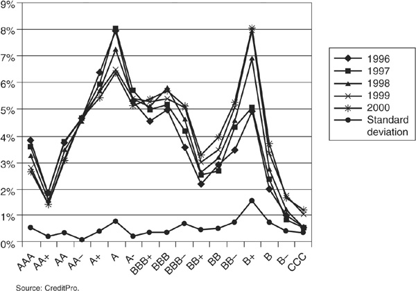
FIGURE 3-17b
Standard & Poor’s Rating Universe
 Another doubtful assumption is the idea of a central tendency. According to this a priori assumption, the distribution of scores is a function of a driving parameter (the central tendency), which is linked to the economic cycle. The central tendency plays the role of a mean around which the distribution of scores is centered: When the economy is in recession, all the distribution is “shifted” toward the right (bad scores), and conversely in expansion. This again is contradicted by Standard & Poor’s experience as low ratings are much more volatile than high ratings.31 Therefore, a simple shift around a central tendency cannot replicate the impact of the business cycle on the distribution of scores or ratings: Both the mean and the volatility change. As a result, calibrations based on the idea of central tendency adjustment would typically underestimate the impact of the cycle on the non-investment-grade universe and penalize investment-grade obligors.
Some Observations about Performance Measures
In many sectors where statistical pattern recognition is applied, classification measures may be sufficient. This is not the case for credit scoring where the assessment of the default risk of an obligor or a loan is associated with its pricing. The question is not how well a specific company is doing compared with some others, but what the probability is of this company defaulting over a given horizon and what would be the impact of this default on the profit of the bank.
Is classification worthless? The answer is no, because classification measures, and ROC in particular, give good insight into Type I and Type II errors. This piece of information matters for bankers and investors for several reasons, such as defining the default cutoff point or enabling them to compare Type I errors for different models—in other words, to assess the rank-ordering accuracy of different models.
Is classification sufficient? No again, because a credit scoring model with good rank-ordering accuracy can prove very imprecise in prediction and seriously damage the profit of the user. Classification measures should therefore be complemented by maximum likelihood or techniques including the utility function of the user.
How to Select a Class of Models?
Fifteen years ago the level of sophistication of credit scoring models was fairly low. One would typically have hesitated between a logit model and a linear discriminant model. With the development of many new techniques and tools such as those reviewed in this chapter, the choice now becomes more complex.
Several factors are important to the choice of a particular class of model over another:
 Performance—the primary factor. A more complex model should provide significantly improved detection or classification of risky firms over a naïve rule. Defining classification or prediction as the goal will have an impact on the choice.
 Data availability and quality. Many models perform well in the laboratory but do not cope with practical difficulties such as missing values or outliers. A simpler but more robust model may be preferable to a state-of-the-art system on patchy data sets.32
 Understanding by users. Users of the scoring models should understand perfectly how the model works and what drives the results. Otherwise they will not be able to spot systematic bias or to understand the limits of their model.
 The robustness of the model to new data. Some models trained on a given data set will provide very different results if the data set is increased slightly. This instability should be avoided, as it may mean that the model is detecting local optima rather than global optima.
 The time required to calibrate or recalibrate a model. This also matters, depending on what frequency the user wants to use to run the model.
It is always advisable not to trust a single model blindly but to run the estimations on the same data set using several models. Significant differences in the outcomes of the different methodologies should lead the user to reassess the performance of the preferred model and to test for potential systematic biases or model risk. Back-testing the results of the model is also very important. Frequently, scoring models will be calibrated on a growth period for example, significantly underestimating the risk of the scored universe in times of recession. Note that, as shown above, ROC or CAP measures will not necessarily detect this because the rank ordering of the model may remain satisfactory. The models should therefore be estimated on a sufficiently long history of data with as many different economic conditions as possible, and the user should use several performance measures based on both classification and prediction.
CONCLUSION
Default risk analysis is obviously the cornerstone of credit risk measurement and management. The quality of the quantitative tools used to perform creditworthiness assessments is critical in order to minimize model risk and to improve the performance of banks.
Being able to develop, update, and improve such quantitative tools is becoming a key requirement for banks, and as we saw in this chapter, there have been significant recent developments in the field of statistical pattern recognition. In addition to the current methodological race, banks are facing data issues. The quality of any system is indeed highly correlated with the value of the related input information. Optimizing and filtering the breadth of the information flow available for modeling is the second pillar for a predictive tool.
APPENDIX 3A
The Effect of Incomplete Information
Duffie and Lando (2001) stress the fact that structural models are based on accounting information. To investors, this information can be somewhat opaque and sometimes insufficient, as we have observed during 2002–2003 with Enron, Worldcom, Parmalat, and others. In addition, accounting practices lead to the release of data with a time lag and in a discrete way. For all these reasons, part of the information used as input in structural models is imperfect.
Duffie and Lando (2001) suggest that if the information available to investors were perfect, then observed credit spreads would be closer to theoretical ones, as predicted by the Merton models. However, as the information available in the financial markets is not complete, observed spreads exhibit significant differences (see Figure 3A-1).
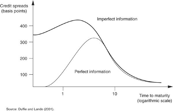
FIGURE 3A-1
Credit Spreads and Information
APPENDIX 3B
A Recipe for an Optimal Selection of Credit Factors in a Linear Logit Scoring Model with Overfitting Regularization
1. Gather a large data set of companies, including the companies’ identifier, the date of financial statements, the date of default if applicable, financial statements, and nonfinancial quantitative information.
2. Transform the data in order to treat outliers appropriately.
3. Build as many credit factors as possible (from 50 to 100). Favor ratios that make economic sense.
4. Do a first cut of credit factors by eliminating, one by one, ratios that contribute the least to the predictive power (GMP) or the accuracy (Gini coefficient) of the 100-factor model. Select the best 20 to 30 factors.
5. Reduce the number of credit factors again. The objective is to limit the list to only 10 factors, taking into consideration their correlation, economic sense, and monotonicity at the same time. The process is as follows:
a. Fit a model based on the best 20 to 30 credit factors, and calculate the PDs for each observation.
b. Group and order the selected ratios into seven main categories:
 Leverage
 Asset utilization
 Profitability
 Liquidity
 Size
Size
 Efficiency
 Structure of balance sheet
c. At the end of the selection process, check to be sure that there are credit factors in at least five different categories.
6. Based on the analysis of monotonicity and correlation, reduce the number of factors to 10 by eliminating nonmonotonic or nonsensical credit factors and those that are highly correlated to others.
7. Run the new model with the 10 factors using the whole sample of transformed factors, and compare with the previous using both GMP and Gini.
8. Review the signs of the weights for each credit factor, and check for economic nonsensicality.
APPENDIX 3C
Key Empirical Considerations about Performance Assessment
Screening in three directions should be performed prior to any formal performance assessment: data issues, discriminability, and stability.
DATA ISSUES
Before looking at sophisticated measurement formulas for the performance of a model, it is very important to assess the quality of the underlying data. Several criteria have to be looked at and reviewed carefully. Four are crucial:
 Use of a large data set
 Availability of a sufficiently high number of defaulted companies
 Presence of a limited number of missing values among selected credit factors
 Recourse to a transparent and “noninvasive” procedure regarding the elimination of outliers
PRACTICAL DISCRIMINABILITY
This concept refers to how well a scoring system classifies unseen data. Practically, the main issue is to maximize the divergence or separation between categories such as default/nondefault. The main problem is to obtain an error rate independent from the set on which it is calculated.33 The error rate will tend to differ when calculated on a training set or a testing set.34 There are four common types of procedures for deriving error rates:
 The holdout estimate method. The sample is split in two exclusive sets. The training set is used for training (minimization of in-sample error), and the testing set is used for performance calculation (calculation of out-of-sample error). This estimate is pessimistically biased: It will typically overestimate the true level of error, as shown in Figure 3C-1. In this respect the size of the training set is important to reduce the bias. The speed of convergence will typically vary with the kind of scoring model used. Defining the appropriateness of a scoring model like a logit, rather than any others such as a probit or a k-nearest neighbor, will depend on the highest obtained speed of convergence, given the fixed amount of data available.
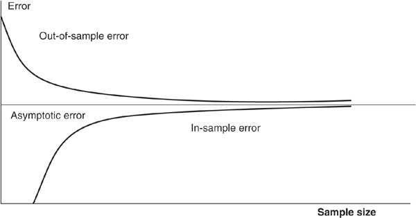
FIGURE 3C-1
In-Sample and Out-of-Sample Performance versus Sample Size
 The n-fold cross-validation technique. This consists of splitting the sample in n sets. The training is performed on n − 1, and the testing is performed on the remaining one. This is repeated as each set is withheld in turn.
 The jackknife. This procedure is used to reduce the bias of the apparent error rate.35
 The bootstrap technique.36 This type of procedure provides non-parametric estimates of the bias and variance of the error rate estimator, thanks to new sets of observation generated by the technique. Bootstrap estimates can display a lower variance than other methods.
Golfarelli, Maio, and Maltoni (1997) consider a reject rate corresponding to a classification made with a confidence level that is too low. The classifier is generally not doing very well when the observed case falls close to the decision-rule boundary, the region where the two classes overlap. Therefore, instead of assigning the case to one of the categories, introducing a reject option reduces the error rate. The larger the reject rate, the smaller the error rate. A good way to define an optimal reject rate is to consider the trade-off, and related costs, between reject and incorrect decision.
STABILITY
This concept is related to optimization. When a user develops a model, either parametric or nonparametric, she will try to obtain unique optimal results, independent from the data set on which it is used.
 For parametric models, this means selecting the most meaningful classes or credit factors. This means also allocating optimal weights to the selected factors. Being able to reach a clear, unique optimal result—and not just a local optimal solution—is a very important issue that requires specific testing.
 For parametric and nonparametric models, this means reviewing carefully the treatment and the impact of outliers on the model. Very straightforward methods exist, such as removing all extreme data that are outside the homogeneous sample, i.e., at a distance of more than two or three times the standard deviation.37 Another technique, called “winsorisation,” consists of bringing back extreme values at a defined level mentioned above. More sophisticated mathematical methods, using the properties of wavelets, have recently been developed. They seem to apply more to large time series at the moment, but they could be used in a cross-sectional way. See Struzik and Siebes (2002).
APPENDIX 3D
Incorporating Costs of Misclassification
We have seen that Bayes’ rule for classification allocated the same cost to Type I and Type II errors. An observation x will be assigned to class ω1 (good firm) if

and to ω2 (bad firms) otherwise.
Figure 3-15 showed how the minimum-loss point could be found—as the point at which the ROC curve is tangential to the iso-loss line with slope p(ω2)/p(ω1).
ROC is also able to deal with asymmetric misclassification costs. The classification rule is changed to

where cij is the cost of assigning x to ωj when it is in ωi. In the case of a credit risk model, c12 (the cost of not detecting a defaulting firm) is likely to be much higher than c21 (the cost of wrongly classifying a good firm in the bad category).
The equation of the iso-loss line is given by  EI, where p(ωi) corresponds to the ex ante belief. The slope of the iso-loss curves is now

The minimum-loss solution is still the point at which the ROC curve and one of the iso-loss lines are tangential.38 Figure 3D-1 illustrates how the move from weighting Type I and Type II errors equally to different costs changes the minimum-loss point.

FIGURE 3D-1
Minimum-Loss Points When Costs Change
A PRACTICAL EXAMPLE ABOUT THE IMPORTANCE OF MISCLASSIFICATION COSTS
Let us consider two travelers with different utility functions using the same airline company. They have to go through the same security control process. This security control process corresponds to the classifier and has to select genuine travelers from criminals.
We consider four models or classifiers:
 Model M1 is performing well in terms of minimum error: low Type I error and low Type II error.
 Model M2 is not performing well: high Type I error and high Type II error.
 Model M3 has mixed performance: high Type I error and low Type II error.
 Model M4 also has mixed performance: low Type I error and high Type II error.
The security systems have a trade-off between speed of processing (i.e., reducing the length of time the passengers will have to wait before boarding) and accuracy in selection (spotting all potential weapons). Type I error corresponds to letting potential criminals through, while Type II error is stopping genuine tourists for further investigation. Models with high Type I errors (M2 and M3) will be unsafe, and models with high Type II errors (M2 and M4) will induce large delays.
The two passengers we consider are one tourist and one patient going for an urgent heart operation. Table 3D-1 summarizes the payoffs for the two passengers.
TABLE 3D-1

From this example we see that it is very difficult to evaluate the performance of the four models independently from the requirement of the users. Obviously M1 will be preferred by both travelers, and M2 will be the least popular choice. However, the choice between M3 and M4 which corresponds to the choice between more Type I errors and more Type II errors depends on the utility of the user.
This shows that ROC curves will not provide sufficient information to qualify fully the performance of any model. The characteristics (cost-benefit) of the user of the models have to be expressed and integrated into the performance measurement.
 , the value of the firm is the sum of the values of its securities:
  . In the Merton model, it is assumed that bondholders cannot force the firm into bankruptcy before the maturity of the debt. At the maturity date T, the firm is considered solvent if its value is sufficient to repay the principal of the debt. Otherwise the firm defaults.
 . Default occurs if the value of the firm is insufficient to repay the debt principal:
  . In that case bond-holders have priority over shareholders and seize the entire value of the firm VT. Otherwise (if
  ) bondholders receive what they are due: the principal K. Thus their payoff is P(T,T) = min(K,VT) = K − max(K−VT,0) (see
 falls in the hands of shareholders. The payoff to equity holders is therefore max
 (see
(see 

 denotes the cumulative normal distribution and r the riskless interest rate.
 The capital structure is simplistic: equity + one issue of zero-coupon debt.

 billion. Assume further that we have solved for A0 = $12.511 billion and
  percent. Finally
  percent, the firm does not pay dividends, and the credit horizon is 1 year. Then


 to denote the function mapping the DD to EDFs.


 is the vector of observations of the random variables
  .
. .
.


 and to group ω2 if
  .
. , then there is high risk; otherwise no. The more significant the difference, the higher the risk (
 , is the score function. Once α is chosen, Fisher’s rule provides a clear-cut segregation between ω1 and ω2. It does not provide probabilities of being in one class or another, conditional on observing realizations of the variables.
 , this means that the probability of being in class ω2 (for example, default) conditional on observing realizations of the variables x (for example, financial ratios


 ; otherwise assign it to ω2. The estimation of w is performed using maximum-likelihood techniques. The larger the training sample on which the weights are estimated, the closer it is from the unknown true value.


 , the transformation is concave; if
  , it becomes convex.
 . Looking at the six nearest neighbors of the new firm (those within the circle), we can see that four of them are good firms and only two are bad firms. The new borrower will therefore be classified as good.
 , corresponding to leverage and ROA) of a given firm we want to classify: x1, x2,…, xp and that the corresponding values for a firm in the training set are y1, y2,…, yp. The Euclidian distance between the two firms is
 distances should be calculated in order to determine the nearest neighbors (the number of variables p may be large as well). For a reasonable data set of SMEs of 10,000 firms, it involves the calculation of nearly 50 million distances. Manipulations of the patterns in the training set to reduce the time and space complexity have therefore been introduced by several authors.
 in the example above, we would have assigned the new borrower to the class of bad firms. In case k is too small, the classification may be unstable. Conversely, if it is really too large, some valuable information may be lost. Enas and Choi (1986) give a rule of
  , but there is no generally accepted best k.

 . If we consider a set of training observations xi, where i ∈ {1,…,n}, an observation xi will be assigned to class ω1 according to the rule
  and to class ω2 according to the rule
  .
. for all i, where
  if
if  and −1 otherwise.
 , where c is the distance from the BSH to the tangent hyperplanes (called canonical hyper-planes).
 , where Fi is a positive parameter that measures the degree of fuzziness or slackness of the rule.
 .
. . The optimization program should include a cost function that penalizes the misclassified observations. Given that misclassification implied large values of Fi, we can adopt a simple rule such as, for example, to make the cost proportional to the sum of adjustments
  .
. for all i. This defines now the best separating surface.
 and the polynomial kernel of order
  . For most kernels it is generally possible to find values for the kernel parameter for which the classes are separable, but there is a risk of overfitting the training data.

 . If an observed measurement x is in Ωi, then it is said to belong to class ωi. The probability of each class occurring is known: p(ω1),…, p(ωC).
 .
.


 was the greatest.
 .
. corresponding to the false nondefaulting companies
 corresponding to the false defaulting companies
 is the specified false alarm rate chosen by the user.


 and the analyst chooses a cutoff level T such that the firm is considered bad if
  and good if
  .
.


 , where E and F are the areas depicted in
  on
on  .
.
 ), for which a probability of default p(xi) is assigned by the model.
 percent to all defaulting companies and
  percent to all nondefaulting companies. Therefore GMP would be 100 percent.
 , where k is the number of parameters, N the size of the sample, and
  the k-dimensional vector of parameter estimates. L(.) is the likelihood function.
 (e.g., rating classes), we obtain
 degrees of freedom.
 It defines a level
  that determines the rejection of the null hypothesis
  (i.e., the hypothesis according to which the data sample follows the identified probability distribution function) is rejected at the α confidence level if
  .
.
 degrees of freedom is 16.9. As the latter is significantly inferior to the statistic, it means that the hypothesis of the scoring system replicating the expected default rate satisfactorily should be rejected.
 . An empirical step distribution function is then built:
 .
.
 is the cutoff value that depends on the confidence level α chosen for the test.
 . Naturally
 . The investor’s view of the true probability (i.e., the probability derived from his model) is qy.


 , which implies that model 2 outperforms model 1.


 EI, where p(ωi) corresponds to the ex ante belief. The slope of the iso-loss curves is now
