6

Tree-level amplitudes

We are now ready to study string interactions. In this chapter we consider the lowest order amplitudes, coming from surfaces with positive Euler number. We first describe the relevant Riemann surfaces and calculate the CFT expectation values that will be needed. We next study scattering amplitudes, first for open strings and then for closed. Along the way we introduce an important generalization in the open string theory, the Chan–Paton factors. At the end of the section we return to CFT, and discuss some general properties of expectation values.

6.1    Riemann surfaces

There are three Riemann surfaces of positive Euler number: the sphere, the disk, and the projective plane.

The sphere

The sphere S₂ can be covered by two coordinate patches as shown in figure 6.1. Take the disks |z| < and |u| < for > 1 and join them by identifying points such that

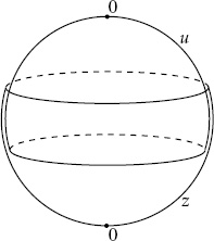
Fig. 6.1.   The sphere built from z and u coordinate patches.

In fact, we may as well take → ∞. The coordinate z is then good everywhere except at the ‘north pole,’ u = 0. We can work mainly in the z patch except to check that things are well behaved at the north pole.

We can think of the sphere as a Riemann surface, taking the flat metric in both patches and connecting them by a conformal (coordinate plus Weyl) transformation. Or, we can think of it as a Riemannian manifold, with a globally defined metric. A general conformal gauge metric is

Since dzd = |z|⁴dud, the condition for the metric to be nonsingular at u = 0 is that exp(2(z,)) fall as |z|⁻⁴ for z → ∞. For example,

describes a sphere of radius r and curvature R = 2/r².

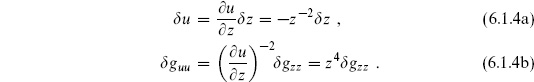
According to the general discussion in section 5.2, the sphere has no moduli and six CKVs, so that in particular every metric is (diff × Weyl)-equivalent to the round metric (6.1.3). Let us see this at the infinitesimal level. As in eq. (5.2.8) one is looking for holomorphic tensor fields g_zz(z) and holomorphic vector fields z(z). These must be defined on the whole sphere, so we need to consider the transformation to the u-patch,

Any holomorphic quadratic differential g_zz would have to be holomorphic in z but vanish as z⁻⁴ at infinity, and so must vanish identically. A CKV z, on the other hand, is holomorphic at u = 0 provided it grows no more rapidly than z² as z → ∞. The general CKV is then

with three complex or six real parameters as expected from the Riemann–Roch theorem.

These infinitesimal transformations exponentiate to give the Möbius group

for complex , , , . Rescaling , , , leaves the transformation unchanged, so we can fix − = 1 and identify under an overall sign reversal of , , , . This defines the group PSL(2, C). This is the most general coordinate transformation that is holomorphic on all of S₂. It is one-to-one with the point at infinity included. Three of the six parameters correspond to ordinary rotations, forming an SO(3) subgroup of PSL(2, C).

The disk

It is useful to construct the disk D₂ from the sphere by identifying points under a reflection. For example, identify points z and z′ such that

In polar coordinates z = rⁱ, this inverts the radius and leaves the angle fixed, so the unit disk |z| ≤ 1 is a fundamental region for the identification. The points on the unit circle are fixed by the reflection, so this becomes a boundary. It is often more convenient to use the conformally equivalent reflection

The upper half-plane is now a fundamental region, and the real axis is the boundary.

The CKG of the disk is the subgroup of PSL(2, C) that leaves the boundary of the disk fixed. For the reflection (6.1.8) this is just the subgroup of (6.1.6) with , , , all real, which is PSL(2, R), the Möbius group with real parameters. One CKV is the ordinary rotational symmetry of the disk. Again, all metrics are equivalent — there are no moduli.

The projective plane

The projective plane RP₂ can also be obtained as a ₂ identification of the sphere. Identify points z and z′ with

These points are diametrically opposite in the round metric (6.1.3). There are no fixed points and so no boundary in the resulting space, but the space is not oriented. One fundamental region for the identification is the unit disk |z| ≤ 1, with points ⁱ and −ⁱ identified. Another choice is the upper half-z-plane. There are no moduli. The CKG is the subgroup of PSL(2, C) that respects the identification (6.1.9); this is just the ordinary rotation group SO(3).

Both the disk and projective plane have been represented as the sphere with points identified under a ₂ transformation, or involution. In fact, every world-sheet can be obtained from a closed oriented world-sheet by identifying under one or two ₂s. The method of images can then be used to obtain the Green’s functions.

6.2    Scalar expectation values

The basic quantities that we need are the expectation values of products of vertex operators. In order to develop a number of useful techniques and points of view we will calculate these in three different ways: by direct path integral evaluation, by using holomorphicity properties, and later in the chapter by operator methods.

The path integral method has already been used in section 5.3 for the Faddeev–Popov determinant and in the appendix for the harmonic oscillator. Start with a generating functional

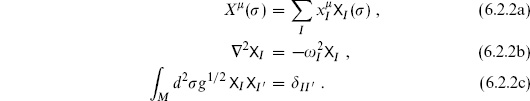
for arbitrary J(). For now we work on an arbitrary compact two-dimensional surface M, and in an arbitrary spacetime dimension d. Expand X () in terms of a complete set _I (),

Then

where

The integrals are Gaussian except for the constant mode

which has vanishing action and so gives a delta function. Carrying out the integrations leaves

As discussed in section 2.1 and further in section 3.2, the timelike modes give rise to wrong-sign Gaussians and are defined by the contour rotation¹ , I 0. The primed Green’s function excludes the zero mode contribution,

It satisfies the differential equation

where the completeness of the _I has been used. The ordinary Green’s function with a delta function source does not exist. It would correspond to the electrostatic potential of a single charge, but on a compact surface the field lines from the source have no place to go. The term can be thought of as a neutralizing background charge distribution.

The sphere

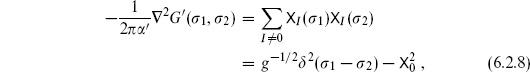
Specializing to the sphere, the solution to the differential equation (6.2.8) is

where

The constant k is determined by the property that G′ is orthogonal to ₀, but in any case we will see that the function drops out of all expectation values. It comes from the background charge, but the delta function from the zero-mode integration forces overall neutrality, , and the background makes no net contribution.

Now consider the path integral with a product of tachyon vertex operators,

This corresponds to

The amplitude (6.2.6) then becomes

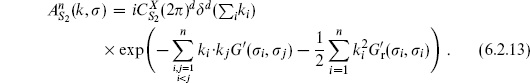
The constant here is

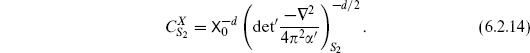
The determinant can be regularized and computed, but we will not need to do this explicitly. We are employing here the simple renormalization used in section 3.6, so that the self-contractions involve

Note that

is finite by design. The path integral on the sphere is then

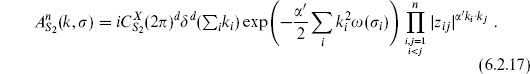
The function has dropped out as promised. The dependence on the conformal factor () is precisely that found in section 3.6 from the Weyl anomaly in the vertex operator. It will cancel the variation of g^1/2 for an on-shell operator.² We can take a metric that is flat in a large region containing all the vertex operators (‘pushing the curvature to infinity’) and the term in (_i) drops out.

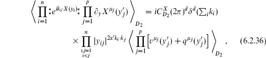
Higher vertex operators are exponentials times derivatives of X , so we also need

This is given by summing over all contractions, where every X or X must be contracted either with an exponential or with another X or X. The XX contraction is simply −′ ln |z|², the s again dropping out in the final expression. The result can be summarized as

Here

come from the contractions with the exponentials. The expectation values of q = X − are given by the sum over all contractions using −(z − z′)⁻² ′ / 2, and those of by the conjugate.

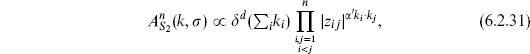
Now we repeat the calculation in a different way, using holomorphicity. As an example consider

The OPE determines this to be

where g(z₁, z₂) is holomorphic in both variables. In the u-patch,

so the condition of holomorphicity at u = 0 is that expectation values of _zX fall as z⁻² at infinity. More generally, a tensor of weight (h, 0) must behave as z^−2h at infinity. Focusing on the z₁-dependence in eq. (6.2.22) at fixed z₂, this implies that g(z₁, z₂) falls as at infinity and so vanishes by holomorphicity. This determines the expectation value up to normalization. Comparing with the path integral result (6.2.19), there is agreement, though the normalization 1 _S2 is seen to diverge as (0). This is just the zero-mode divergence from the infinite volume of spacetime.

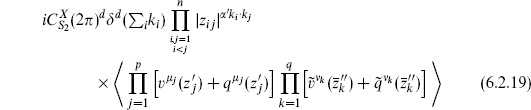
To obtain the expectation value of the product of vertex operators

by this method is less direct, because the exponentials are not holomorphic. In fact they can be factored into holomorphic and antiholomorphic parts, but this is subtle and is best introduced in operator language as we will do in chapter 8. We use the holomorphicity of the translation current. Consider the expectation value with one current X (z) added. The OPE of the current with the vertex operators determines the singularities in z,

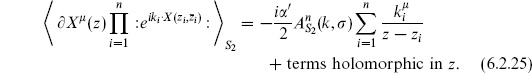
Now look at z → ∞. The condition that _u X be holomorphic at u = 0 again requires that the expectation value vanish as z⁻² when z → ∞. The holomorphic term in eq. (6.2.25) must then vanish, and from the vanishing of the order z⁻¹ term we recover momentum conservation,

Let us also say this in a slightly different way. Consider the contour integral of the spacetime translation current

where the contour C encircles all the exponential operators. There are two ways to evaluate this. The first is to contract C until it is a small circle around each vertex operator, which picks out the (z − z_i)⁻¹ term from each OPE and gives . The second is to expand it until it is a small circle in the u-patch: by holomorphicity at u = 0 it must vanish. This sort of ‘contour-pulling’ argument is commonly used in CFT.

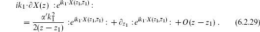
We have used the OPE to determine the singularities and then used holomorphicity to get the full z-dependence. Now we look at the second term of the OPE as z → z₁. Expanding the result (6.2.25) gives

Contracting this with , the term of order (z − z₁)⁰ must agree with the OPE

This implies

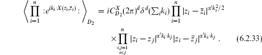
Integrating, and using the conjugate equation and momentum conservation, determines the path integral up to normalization,

in agreement with the first method. Note that to compare we must push the curvature to infinity ((_i) = 0) so that [  ]_r = : :.

It is worth noting that the intermediate steps in the path integral method depend in a detailed way on the particular choice of Riemannian metric. The metric is needed in order to preserve coordinate invariance in these steps. A different, Weyl-equivalent, metric gives a different Laplacian and different eigenfunctions, though at the very end this dependence must drop out in string theory. The second method uses only the basic data of a Riemann surface, its holomorphic structure.

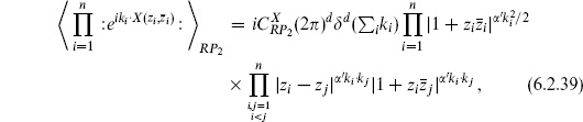
The disk

The generalization to the disk is straightforward. We will represent the disk by taking the above representation of the sphere and restricting z to the upper half of the complex plane. The Neumann boundary term is accounted for by an image charge,

up to terms that drop out due to momentum conservation. Then

For expectation values with _aX s one again sums over contractions, now using the Green’s function (6.2.32). Note that (or ) has a nonzero contraction.

For two points on the boundary, the two terms in the Green’s function (6.2.32) are equal, and the Green’s function diverges at zero separation even after normal ordering subtracts the first term. For this reason, boundary operators must be defined with boundary normal ordering, where the subtraction is doubled:

with y denoting a coordinate on the real axis. The combinatorics are the same as for other forms of normal ordering. Boundary normal-ordered expectation values of boundary operators have the same good properties (nonsingularity) as conformal normal-ordered operators in the interior.

An expectation value with exponentials both in the interior and on the boundary, each having the appropriate normal ordering, is given by taking the appropriate limit of the interior result (6.2.33) and dropping the factor for the boundary operators. Explicitly, for exponentials all on the boundary,

More generally,

where now

and the qs are contracted using −2′ (y − y′)⁻².

The projective plane

The method of images gives the Green’s function as

Now

and so on for more general expectation values. There is no boundary because the involution has no fixed points — there is no way for a point z to approach its image .

6.3    The bc CFT

The sphere

The path integral for the ghosts has already been set up in section 5.3. According to the Riemann–Roch theorem, the simplest nonvanishing expectation value will be

Up to normalization (a functional determinant), the result (5.3.18) was just the zero-mode determinant,

The six CKVs were found in section 6.1. In a complex basis they are

In this basis the determinant splits into two 3 × 3 blocks, and the expectation value becomes

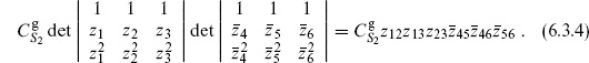
The constant includes the functional determinant and also a finite-dimensional Jacobian (independent of the positions) that arises because the basis (6.3.3) is not orthonormal.

This is the only bc path integral that we will actually need for the tree-level amplitudes, but for completeness we give

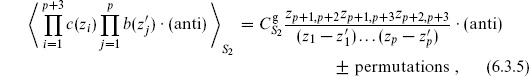
obtained by contracting the bs with cs. The antiholomorphic part ‘anti’ has the same form. We are being a little careless with the overall sign; again, for the Faddeev–Popov determinant we will in any case take an absolute value.

To give an alternative derivation using holomorphicity, we again consider first the conservation law, derived by inserting into the amplitude (6.3.5) the ghost number contour integral _C dz j(z)/2i, where C encircles all the vertex operators and j = − :bc : is again the ghost number current. From the OPE with b and c, this just counts the number of c minus the number of b fields, giving n_c − n_b times the original amplitude. Now pull the contour into the u-patch using the conformal transformation (2.5.17),

The shift +3 comes about because j is not a tensor, having a z⁻³ term in its OPE with T . In the last step we use holomorphicity in the u-patch. The nonzero amplitudes therefore have n_c − n_b = 3 and similarly n − n = 3, in agreement with the Riemann–Roch theorem.

From the OPE, the ghost expectation value (6.3.1) is holomorphic in each variable, and it must have a zero when two identical anticommuting fields come together. Thus it must be of the form

with F holomorphic and antiholomorphic functions of the positions. As z₁ → ∞ this goes as . However, c is a tensor of weight −1, so the amplitude can be no larger than at infinity. Thus F(z_i) must be independent of z₁, and so also of z₂ and z₃; arguing similarly for we obtain again the result (6.3.4). The same argument gives for the general case (6.3.5) the result

which has the correct poles, zeros, and behavior at infinity. The permutations (6.3.5) evidently sum up to give this single term.

We have considered the =2 theory that is relevant to the ghosts of the bosonic string, but either method generalizes readily to any .

The disk

The simplest way to obtain the bc amplitudes on the disk is with the doubling trick. As in eq. (2.7.30), we can represent both the holomorphic and antiholomorphic fields in the upper half-plane by holomorphic fields in the whole plane, using

The expectation value of the holomorphic fields follows as on the sphere,

for all z. Then for example

More general correlators are obtained in the same way.

The projective plane

The doubling trick again can be used. The involution implies that

Again

and so

6.4    The Veneziano amplitude

Open string amplitudes are slightly simpler than closed string amplitudes, so we begin with these.

We represent the disk as the upper half-plane so the boundary coordinate y is real. There are no moduli. After fixing the metric, the CKG PSL(2, R) can be used to fix the three vertex operators to arbitrary positions y₁, y₂, y₃ on the boundary, except that this group does not change the cyclic ordering of the vertex operators so we must sum over the two orderings. For three open string tachyons on the disk, the general expression (5.3.9) for the string S-matrix thus reduces to

each fixed coordinate integration being replaced by the corresponding c-ghost. Each vertex operator includes a factor of g_o, the open string coupling. The factor ⁻ is from the Euler number term in the action. Of course g_o and are related, , but we will determine the constant of proportionality as we go along.

The expectation values in (6.4.1) were found in the previous sections (again, we take the absolute value for the ghosts), giving

where . Momentum conservation and the mass-shell condition imply that

and the same for the other k_i · k_j, so this reduces to

This is independent of the gauge choice y_i, which is of course a general property of the Faddeev–Popov procedure. The Weyl invariance is crucial here — if the vertex operators were taken off the mass shell, the amplitude would depend on the choice of y_i.

We could have used independence of the y_i to determine the Faddeev–Popov determinant without calculation. Using the mass-shell condition and momentum conservation, the X expectation value is proportional to |y₁₂ y₁₃ y₂₃|⁻¹, and so the measure must be reciprocal to this. This same measure then applies for n > 3 vertex operators, because in all cases three positions are fixed.

The four-tachyon amplitude is obtained in the same way,

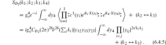
This is again independent of y_1,2,3 after a change of variables (a Möbius transformation) on y₄. It is convenient to take y₁ = 0, y₂ = 1, and y₃ → ∞. The amplitude is conventionally written in terms of the Mandelstam variables

These are not independent: momentum conservation and the mass-shell condition imply that

Using 2′k_i · k_j = −2 + ′ (k_i + k_j)², the amplitude becomes

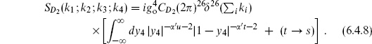
The integral splits into three ranges, −∞ < y₄ < 0, 0 < y₄ < 1, and 1 < y₄ < ∞. For these three ranges the vertex operators are ordered as in figures 6.2(a), (b), and (c) respectively. Möbius invariance can be used to take each of these ranges into any other, so they give contributions that are equal up to interchange of vertex operators. The (t ↔ s) term gives figures 6.2(d), (e), and (f). In all,

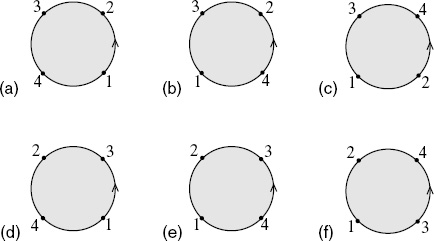
Fig. 6.2.   The six cyclically inequivalent orderings of four open string vertex operators on the disk. The coordinate y increases in the direction of the arrow, except that at point 3 it jumps from +∞ to −∞

where

The three terms come from figures 6.2(c), (f), 6.2(b), (d), and 6.2(a), (e) respectively.

The integral I(s, t) converges if ′s < − 1 and ′t < −1. As ′s → −1, the integral diverges at y = 0. To study the divergence, take a neighborhood of y = 0 and approximate the integrand:

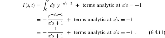
In (6.4.11), we have evaluated the integral in the convergent region. We see that the divergence is a pole at s = −1/′ , the mass-squared of the open string tachyon. The variable s is just the square of the center-of-mass energy for scattering 1 + 2 → 3 + 4, so this pole is a resonance due to an intermediate tachyon state. Again, it is an artifact of the bosonic string that this lightest string state is tachyonic, and not relevant to the discussion. The pole is due to the process shown in figure 6.3(a), in which tachyons 1 and 2 join to become a single tachyon, which then splits into tachyons 3 and 4.

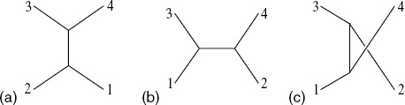
Fig. 6.3.   Processes giving poles in the (a) s-, (b) t-, and (c) u-channels.

Because the singularity at ′s = −1 is just a pole, I(s, t) can be analytically continued past this point into the region ′s > −1. The amplitude is defined via this analytic continuation. The divergence of the amplitude at the pole is an essential physical feature of the amplitude, a resonance corresponding to propagation of the intermediate string state over long spacetime distances. The divergence of the integral past the pole is not; it is just an artifact of this particular integral representation of the amplitude. The continuation poses no problem. In fact, we will see that every string divergence is of this same basic form, so this one kind of analytic continuation removes all divergences — except of course for the poles themselves. The pole is on the real axis, so we need to define it more precisely. The correct prescription for a Minkowski process is

where P denotes the principal value. Unitarity (which we will develop more systematically in chapter 9) requires this pole to be present and determines its coefficient in terms of the amplitude for two tachyons to scatter into one:

Gathering together the factors in the four-tachyon amplitude, including an equal contribution to the pole from I(u, s), and using the three-tachyon result (6.4.4), the condition (6.4.13) gives

The three-tachyon amplitude is then

The various functional determinants have dropped out. Using unitarity, all normalizations can be expressed in terms of the constant g_o appearing in the vertex operators. The determinants can in fact be computed by careful regularization and renormalization, and the relative normalizations of different topologies agree with those from unitarity.

Continuing past the pole, we encounter further singularities. Taylor expanding the integrand at y = 0 gives

The second term gives a pole at ′s = 0,

From the further terms in the Taylor expansion, the amplitude has poles at

These are precisely the positions of the open string states. The integral I(s, t) also has poles in the variable t at the same positions (6.4.18), coming from the endpoint y = 1. These are due to the process of figure 6.3(b). The other two terms in the amplitude (6.4.9) give further contributions to the s- and t-channel poles, and also give poles in the u-channel, figure 6.3(c). Because the residue at s = 0 in (6.4.17) is odd in u − t, this pole actually cancels that from I(s, u), as do all poles at even multiples of 1/′. This will not be true for the more general open string theories to be introduced in the next section.

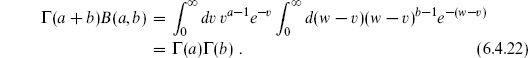
Define the Euler beta function

so that

This can be expressed in terms of gamma functions. Defining y = / w for fixed w gives

Multiplying both sides by ^−w, integrating , and regrouping gives

The four-tachyon amplitude is then

where

This is the Veneziano amplitude, originally written to model certain features of strong interaction phenomenology.

The high energy behavior of the Veneziano amplitude is important. There are two regions of interest, the Regge limit,

and the hard scattering limit,

If we consider the scattering process 1 + 2 → 3 + 4 (so that and are positive and and negative), then in the 1-2 center-of-mass frame,

where E is the center-of-mass energy and is the angle between particle 1 and particle 3. The Regge limit is high energy and small angle, while the hard scattering limit is high energy and fixed angle. Using Stirling’s approximation, Γ( + 1) ^–(2 )^1/2, the behavior in the Regge region is

where again _o(t) = ′t + 1. That is, the amplitude varies as a power of s, the power being t-dependent. This is Regge behavior. At the poles of the gamma function, the amplitude is an integer power of s, corresponding to exchange of a string of integer spin _o(t).

In the hard scattering limit,

where

is positive. The result (6.4.29) is notable. High energy, fixed angle scattering probes the internal structure of the objects being scattered. Rutherford discovered the atomic nucleus with hard alpha–atom scattering. Hard electron–nucleon scattering at SLAC revealed the quark constituents of the nucleon. In quantum field theory, hard scattering amplitudes fall as a power of s. Even a composite object like the nucleon, if its constituents are pointlike, has power law amplitudes. The exponential falloff (6.4.29) is very much softer. The result (6.4.29) suggests a smooth object of size ′^1/2, as one would expect.

We started with the three-particle amplitude, skipping over the zero-, one-, and two-particle amplitudes. We will discuss these amplitudes, and their interpretation, in section 6.6.

6.5    Chan–Paton factors and gauge interactions

In this section we will consider the interactions of the massless vector state of the open string. To make the discussion a bit more interesting, we first introduce a generalization of the open string theory.

At the end of chapter 3 we introduced a very large class of bosonic string theories, but in this first look at the interactions we are focusing on the simplest case of 26 flat dimensions. One can think of this in terms of symmetry: this theory has the maximal 26-dimensional Poincaré invariance. In the closed bosonic string this is the unique theory with this symmetry. An outline of the proof is as follows. The world-sheet Noether currents for spacetime translations have components of weights (1, 0) and (0, 1). By an argument given in section 2.9, these currents are then holomorphic in z or . We have seen in the calculations in this chapter that this is enough to determine all the expectation values.

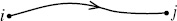
Fig. 6.4.   Open string with Chan–Paton degrees of freedom.

In open string theory, however, there is a generalization. The open string has boundaries, endpoints. In quantum systems with distinguished points it is natural to have degrees of freedom residing at those points in addition to the fields propagating in the bulk. At each end of the open string let us add a new degree of freedom, known as a Chan–Paton degree of freedom, which can be in one of n states. A basis of string states is then

where i and j denote the states of the left- and right-hand endpoints, running from 1 to n. The energy-momentum tensor is defined to be the same as before, with no dependence on the new degrees of freedom. Conformal invariance is therefore automatic. Poincaré invariance is automatic as well, as the Chan–Paton degrees of freedom are invariant. Although these new degrees of freedom have trivial world-sheet dynamics, they will have a profound effect on the spacetime physics.

In string theories of the strong interaction, the motivation for this was to introduce SU(3) flavor quantum numbers: the endpoints are like quarks and antiquarks, connected by a color-electric flux tube. Now we are motivating it in the general framework of considering all possibilities with given symmetries. We will give a new interpretation to the Chan–Paton degrees of freedom in chapter 8, and a possible further refinement in chapter 14.

There are now n² scalar tachyons, n² massless vector bosons, and so forth. The n² Hermitian matrices , normalized to

are a complete set of states for the two endpoints. These are the representation matrices of U(n), so one might guess that the massless vectors are associated with a U(n) gauge symmetry; we will soon see that this is the case.

Define the basis

Now consider the four-tachyon amplitude shown in figure 6.2(a), in which the vertex operators are arranged in the cyclic order 1234. Because the Chan–Paton degrees of freedom do not appear in the Hamiltonian, their state does not evolve between the vertex operators: the right-hand endpoint of tachyon 1 must be in the same state as the left-hand endpoint of tachyon 2, and so forth. Thus, the amplitude 6.2(a) will now contain an additional factor of

from the overlap of the Chan–Paton wavefunctions for each tachyon. This rule generalizes to an arbitrary amplitude: each vertex operator now contains a Chan–Paton factor from the wavefunction of the endpoint degrees of freedom, and the amplitude for each world-sheet is multiplied by a trace of the Chan–Paton factors around each boundary.

The three-tachyon amplitude becomes

the two cyclic orderings now having different Chan–Paton traces. The four-tachyon amplitude is

Considering again the unitarity relation (6.4.13), the pole at s = −1/′ acquires a factor of

on the left and a factor of

on the right, the sum being over the Chan–Paton wavefunction of the intermediate state. The completeness of the and the normalization (6.5.2) imply that

for any matrices A and B, and so the amplitudes are still unitary.

Gauge interactions

The amplitude for a gauge boson and two tachyons is

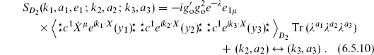
We have used the gauge boson vertex operator (3.6.26), but for now are allowing an independent normalization constant . Using the results of section 6.2, the X path integral is

Using momentum conservation, the mass-shell conditions, and the physical state condition k₁· ₁ = 0, the amplitude becomes

where k_ij ≡ k_i − k_j. This is again independent of the vertex operator positions.

The s = 0 pole in the four-tachyon amplitude no longer vanishes. The terms that canceled now have the Chan–Paton factors in different orders, so the pole is proportional to

Relating the coefficient of this pole to the amplitude (6.5.12) by unitarity, one obtains

This is the same relative normalization as from the state–operator mapping: there is only one independent coupling constant.

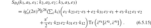
For the three-gauge-boson coupling, a similar calculation gives

Up to first order in the momenta, the amplitudes we have found are reproduced by the spacetime action

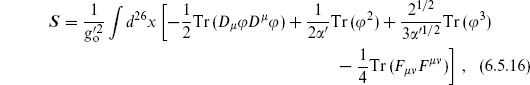
where the tachyon field and the Yang–Mills vector potential A are written as n × n matrices, e. g. . Also, D = − i[A, ] and F = A − A − i[A, A].

This is the action for a U(n) gauge field coupled to a scalar in the adjoint representation. Adding in the Chan–Paton factors has produced just the gauge-invariant expressions needed. The gauge invariance is automatic because the decoupling of unphysical states is guaranteed in string perturbation theory, as we will develop further.

At momenta k small compared to the string scale, the only open string states are the massless gauge bosons. As discussed in section 3.7, it is in this limit that the physics should reduce to an effective field theory of the massless states. We have therefore been somewhat illogical in including the tachyon in the action (6.5.16); we did so for illustration, but now let us focus on the gauge bosons. The four-gauge-boson amplitude has a form analogous to the Veneziano amplitude but with additional structure from the polarization tensors. Expanding it in powers of ′k², the first term, which survives in the zero-slope limit ′ → 0, is the sum of pole terms in s, t, and u plus a constant. Consistency guarantees that it is precisely the four-gauge-boson amplitude obtained in field theory from the Yang–Mills Lagrangian F F. Note, however, the term of order ′k³ in the three-gauge-boson amplitude (6.5.15). This implies a higher derivative term

in the Lagrangian. Similarly, expanding the four-point amplitude reveals an infinite sum of higher order interactions (beyond (6.5.17), these do not contribute to the three-gauge-boson amplitude for kinematic reasons). String loop amplitudes also reduce, in the low energy region, to the loops obtained from the effective Lagrangian. By the usual logic of effective actions, the higher derivative terms are less important at low energy. The scale where they become important, ′k² 1, is just where new physics (massive string states) appears and the effective action is no longer applicable.

If we have a cutoff, why do we need renormalization theory? Renormalization theory still has content and in fact this is its real interpretation: it means that low energy physics is independent of the details of the high energy theory, except for the parameters in the effective Lagrangian. This is a mixed blessing: it means that we can use ordinary quantum field theory to make predictions at accelerator energies without knowing the form of the Planck scale theory, but it also means that we cannot probe the Planck scale theory with physics at particle accelerators.

The string spectrum and amplitudes have an obvious global U(n) symmetry,

which leaves the Chan–Paton traces and the norms of states invariant. From the detailed form of the amplitudes, we have learned that this is actually a local symmetry in spacetime. We will see that this promotion of a global world-sheet symmetry to a local spacetime symmetry is a rather general phenomenon in string theory.

All open string states transform as the n × n adjoint representation under the U(n) symmetry. Incidentally, U(n) is not a simple Lie algebra: U(n) = SU(n) × U(1). The U(1) gauge bosons, _ij = _ij / n^1/2, decouple from the amplitudes (6.5.12) and (6.5.15). The adjoint representation of U(1) is trivial, so all string states are neutral under the U(1) symmetry.

The unoriented string

It is interesting to generalize to the unoriented string. Consider first the theory without Chan–Paton factors. In addition to Möbius invariance, the X CFT on the sphere or disk is invariant under the orientation-reversing symmetry ¹ → − ¹ in the open string or ¹ → 2 − ¹ in the closed string. This world-sheet parity symmetry is generated by an operator Ω. From the mode expansions it follows that

in the open string and

in the closed string. The symmetry extends to the ghosts as well, but to avoid distraction we will not discuss them explicitly, since they only contribute a fixed factor to the tree-level amplitudes.

The tachyon vertex operators are even under world-sheet parity in either the closed or open string (this is obvious for the integrated vertex operators, without ghosts; the fixed operators must then transform in the same way), determining the sign of the operator. All states can then be classified by their parity eigenvalue = ± 1. The relation (6.5.19) in the open string implies that

World-sheet parity is multiplicatively conserved. For example, the three-tachyon amplitude is nonzero, consistent with (+1)³ = 1. On the other hand, the massless vector has = −1 and so we would expect the vector–tachyon–tachyon amplitude (6.5.10) and three-vector amplitude (6.5.15) to vanish in the absence of Chan–Paton degrees of freedom, as indeed they do (the ^a are replaced by 1 and the commutators vanish). The different cyclic orderings, related to one another by world-sheet parity, cancel.

Given a consistent oriented string theory, we can make a new unoriented string theory by restricting the spectrum to the states of = +1. States with odd ′m² remain, while states with even ′m², including the photon, are absent. The conservation of guarantees that if all external states have = +1, then the intermediate states in tree-level amplitudes will also have = +1. Unitarity of the unoriented theory thus follows from that of the oriented theory, at least at tree level (and in fact to all orders, as we will outline in chapter 9).

The main point of interest in the unoriented theory is the treatment of the Chan–Paton factors. Since we have identified these with the respective endpoints of the open string, world-sheet parity must reverse them,

Again, this is a symmetry of all amplitudes in the oriented theory. To form the unoriented theory, we again restrict the spectrum to world-sheet parity eigenvalue = +1. Take a basis for in which each matrix is either symmetric, s^a = +1, or antisymmetric, s^a = −1. Then

The world-sheet parity eigenvalue is = _Ns^a, and the unoriented spectrum is

For the massless gauge bosons the Chan–Paton factors are the n × n antisymmetric matrices and so the gauge group is SO(n). The states at even mass levels transform as the adjoint representation of the orthogonal group SO(n), and the states at odd mass levels transform as the traceless symmetric tensor plus singlet representations.

The oriented theory has a larger set of orientation-reversing symmetries, obtained as a combination of Ω and a U(n) rotation,

We can form more general unoriented theories by restricting the spectrum to = +1, which is again consistent with the interactions. Acting twice with Ω gives

We will insist that for reasons to be explained below. This then implies that

That is, is symmetric or antisymmetric.

A general change of Chan–Paton basis,

transforms to

In the symmetric case, it is always possible to find a basis such that = 1, giving the theory already considered above. In the antisymmetric case there is a basis in which

Here I is the k × k identity matrix and n = 2k must be even because is an invertible antisymmetric matrix. We take a basis for the Chan–Paton wavefunctions such that M(^a)^T M = s^{a′ a} with s^a′ = ±1. Then the world-sheet parity eigenvalue is = _N s^a′, and the unoriented spectrum is

At the even mass levels, including the gauge bosons, this defines the adjoint representation of the symplectic group Sp(k).

The argument that we must have = 1 to construct the unoriented theory is as follows. Since Ω² = 1, it must be that acts only on the Chan–Paton states, not the oscillators. In fact, from eq. (6.5.26), it acts on the Chan–Paton wavefunction as

where the last equality must hold in the unoriented theory, since all states in this theory are invariant under Ω and so also under . Now we assert that the allowed Chan–Paton wavefunctions must form a complete set. The point is that two open strings, by the splitting–joining interaction of figure 3.4(c), can exchange endpoints. In this way one can get to a complete set, that is, to any Chan–Paton state |i j (this argument is slightly heuristic, but true). By Schur’s lemma, if eq. (6.5.32) holds for a complete set, then ^−1T = 1 and so .

We might try to obtain other gauge groups by taking different sets of ^a. In fact, the oriented U(n) and unoriented SO(n) and Sp(k) theories constructed above are the only possibilities. Generalization of the completeness argument in eqs. (6.5.7)–(6.5.9) shows these to be the most general solutions of the unitarity conditions. In particular, exceptional Lie algebras, which are of interest in grand unification and which will play a major role in volume two, cannot be obtained with Chan–Paton factors (in perturbation theory). In closed string theory there is another mechanism that gives rise to gauge bosons, and it allows other groups.

6.6    Closed string tree amplitudes

The discussion of closed string amplitudes is parallel to the above. The amplitude for three closed string tachyons is

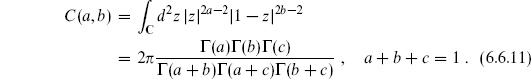
In this case the CKG PSL(2, C) (the Möbius group) can be used to fix the three vertex operators to arbitrary positions z_1,2,3. Taking the expectation values from section 6.2, the result is again independent of the vertex operator positions,

where .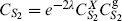

For four closed string tachyons,

where the integral runs over the complex plane C. Evaluating the expectation value and setting z₁ = 0, z₂ = 1, z₃ = ∞, this becomes

where

Here s + t + u = −16/′, but we indicate the dependence of J on all three variables to emphasize its symmetry among them. This amplitude converges when s, t, u < −4/′. It has poles in the variable u from z₄ → 0, in the variable t from z₄ → 1, and in the variable s from z₄ → ∞. The poles are at the values

which are the masses-squared of the closed string states. The pole at ′ s = −4 is

Unitarity gives

and so

Like the Veneziano amplitude, the amplitude for four closed string tachyons can be expressed in terms of gamma functions (exercise 6.10):

where _c() = 1 + ′/4 and

This is the Virasoro–Shapiro amplitude. There is just a single term, with poles in the s-, t-, and u-channels coming from the gamma functions in the numerator. Like the Veneziano amplitude, the Virasoro–Shapiro amplitude has Regge behavior in the Regge limit,

and exponential behavior in the hard scattering limit,

On the sphere, the amplitude for a massless closed string and two closed string tachyons is

where . Expanding the Virasoro–Shapiro amplitude (6.6.10) on the s = 0 pole and using unitarity determines

again in agreement with the state–operator mapping with overall constant g_c. The amplitude (6.6.14) would be obtained in field theory from the spacetime action S + S_T , where S is the action (3.7.20) for the massless fields, and where

is the action for the closed string tachyon T . For example, the amplitude for a graviton of polarization is obtained from this action by expanding

Note that this is the Einstein metric, whose action (3.7.25) is independent of the dilaton. The normalization of the fluctuation is determined by that of the graviton kinetic term in the spacetime action. Specifically, if one takes − = −2 () with = 1, the effective action for has the canonical normalization for a real scalar. The field theory amplitude matches the string result (6.6.14) and relates the normalization of the vertex operators to the gravitational coupling,

The amplitude for three massless closed strings is

where

The order k² terms in this amplitude correspond to the spacetime action (3.7.25), while the k⁴ and k⁶ terms come from a variety of higher derivative interactions, including terms quadratic and cubic in the space-time curvature. These higher corrections to the action can also be determined by calculating higher loop corrections to the world-sheet beta functions (3.7.14).

The tensor structure of the closed string amplitude (6.6.19) is just two copies of that in the open string amplitude (6.5.15), if one sets ′ = 2 in the closed string and ′ = in the open. The same holds for the amplitude (6.6.14). This is a consequence of the factorization of free-field expectation values on the sphere into holomorphic and antiholomorphic parts. A similar factorization holds for four or more closed strings before integration over the vertex operator positions. Further, by careful treatment of the contour of integration it is possible to find relations between the integrated amplitudes. For the four-tachyon amplitudes the integrals above are related

after use of the gamma function identity Γ()Γ(1−) sin() = ; we now indicate the explicit dependence of the integrals on ′. For the general integral appearing in four-point closed string amplitudes there is a relation

This implies a corresponding relation between four-point open and closed string amplitudes

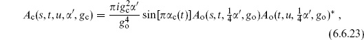
where the open string amplitudes include just one of the six cyclic permutations, with poles in the indicated channels.

Consistency

In chapter 9 we will discuss the convergence and gauge invariance of tree-level amplitudes in a general way, but as an introduction we will now use the OPE to see how these work for the lowest levels. Consider the operator product

This appears in the amplitude with z₁₄ integrated. The integral converges as z₁₄ → 0 when

and has a pole at that point. The coefficient of the pole is just the tachyon vertex operator. Thus, if a pair of tachyons in any amplitude has total momentum (k₁ + k₄)² = 4/′, there will be a pole proportional to the amplitude with one fewer tachyon as required by unitarity. A pole in momentum space corresponds to long distance in spacetime, so this is a process in which two tachyons scatter into one, which then propagates and interacts with the remaining particles. Carrying the OPE further, the O(z₁₄) and O(₁₄) terms do not produce poles because the angular integration gives zero residue, the O(z₁₄₁₄) term gives a massless pole, and so on.

Now let us look a little more closely at the way the local spacetime symmetries are maintained in the string amplitudes. The various amplitudes we have calculated all vanish if any of the polarizations are of the form = k, or = K + K with k · = K · = 0. The corresponding spacetime actions are thus invariant under the Yang–Mills, coordinate, and antisymmetric tensor symmetries. As discussed in section 3.6, the vertex operator for a longitudinal polarization is the sum of a total derivative and a term that vanishes by the equations of motion. Upon integration, the total derivative vanishes but the equation of motion term might have a source at one of the other vertex operators in the path integral. The operator product (6.6.24) vanishes rapidly when k₁ · k₄ is large. Using this property, there will be for any pair of vertex operators a kinematic region in which all possible contact terms are suppressed. The amplitude for any null polarization then vanishes identically in this region, and since all amplitudes are analytic except for poles (and branch points at higher order) the amplitudes for null polarizations must vanish everywhere. We see that the singularities required by unitarity, as well as any possible divergences or violations of spacetime gauge invariance, arise from the limits z → 0, 1, ∞, where two vertex operators come together. For the sphere with four marked points (vertex operators) these are the boundaries of moduli space. The analytic continuation argument used here is known for historic reasons as the canceled propagator argument.

Closed strings on D₂ and RP₂

The lowest order closed–open interactions come from the disk with both closed and open vertex operators. The low energy effective action for these can be deduced from general considerations. With a trivial closed string background we found the usual gauge kinetic term,

Obviously the metric must couple to this in a covariant way. In addition, the coupling of the dilaton can be deduced. Recall that , with Φ₀ the expectation value of the dilaton. So we should replace this (inside the integral) with Φ = Φ₀ + . The action

thus incorporates all interactions not involving derivatives of the closed string fields; indices are now raised and lowered with G. This action reflects the general principle that the effective action from Euler number is weighted by .

The disk and projective plane also make a contribution to purely closed string interactions. The amplitudes for n closed strings are of order , one power of g_c higher than the sphere. Closed string loop amplitudes, to be considered in the next chapter, are of order times the sphere, because emitting and reabsorbing a closed string adds two factors of g_c. Thus the disk and projective plane are ‘half-loop order.’

Of particular interest are the amplitudes on the disk and the projective plane with a single closed string vertex operator. Fixing the position of the vertex operator removes only two of the three CKVs, the residual gauge symmetry consisting of rotations about the vertex operator position. Thus we have to divide the amplitude by the volume of this residual CKG. We have not shown how to do this explicitly, but will work it out for the torus in the next chapter. For the disk with one closed string this is a finite factor and the result is nonzero. The amplitude is a numerical factor times which in turn is a pure number, times powers of ′ as required by dimensional analysis. We will not work out these numerical factors here, but will obtain them in an indirect way in chapter 8.

Thus there is an amplitude for a single closed string to appear from the vacuum, either through the disk or the projective plane, necessarily with zero momentum. Such an amplitude is known as a tadpole. In other words, the background closed string fields are corrected from their original values at order g_c. Again we can write an effective action, which is simply

the Φ dependence deduced as above. This is a potential for the dilaton. We will consider it further in the next chapter.

The amplitude for a single closed string on the sphere, on the other hand, is zero. The residual CKG is a noncompact subgroup of PSL(2, C) and so one has to divide by an infinite volume. A nonzero result would have been a logical inconsistency, a zeroth order correction to the background fields. Similarly the amplitude for two closed strings on the sphere (a zeroth order correction to the mass) vanishes, as do the corresponding disk amplitudes, one or two open strings. The amplitudes with no vertex operators at all are also meaningful — they just calculate the term of order in the Taylor expansion of the action (6.6.28). The disk amplitude with no vertex operators is thus nonvanishing; this requires a somewhat formal treatment of the conformal Killing volume.

6.7    General results

In this section we obtain some general results concerning CFT on the sphere and disk.

Möbius invariance

We have seen that the sphere has a group of globally defined conformal transformations, the Möbius group PSL(2, C),

for complex , , , with − = 1. This is the most general conformal transformation that is one-to-one on all of S₂, the complex z-plane plus the point at infinity. Expectation values must be invariant under any Möbius transformation:

We will consider the consequences of this symmetry for expectation values with one, two, three, or four local operators.

For a single operator of weight (h_i, _i), the rescaling plus rotation z′ = z gives

The one-point function therefore vanishes unless h_i = _i = 0. This is another way to see that the one-point string amplitude vanishes on the sphere, because the matter factor is the expectation value of a (1, 1) operator.

For n = 2, we can use a translation plus z′ = z to bring any pair of operators to the points 0 and 1, giving

so the position dependence is completely determined. Single-valuedness implies that J_i +J_j ∈ , where J_i = h_i − _i. There is a further constraint on the two-point function from the conformal transformation z′ = z + (z − z₁)(z − z₂) + O(²), which leaves z₁ and z₂ fixed. For general operators this is complicated, but for tensor fields and it simply implies that

Any three points z_1,2,3 can be brought to given positions by a Möbius transformation. For n ≥ 3, Möbius invariance therefore reduces the expectation value from a function of n complex variables to a function of n − 3 complex variables. Again the result takes a simple form only for tensor fields. For example, for three tensor fields one finds

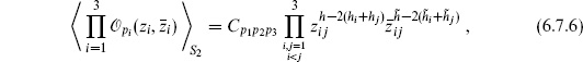
where C_p1p2p3 is independent of position and h = h₁ + h₂ + h₃. For four primary fields,

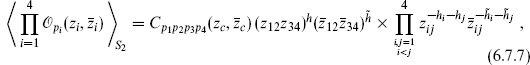
where , and z_c = z₁₂z₃₄/z₁₃z₂₄ is the Möbius invariant cross-ratio. The function C_p1p2p3p4(z_c, _c) is not determined by conformal invariance, so we are reduced from a function of four variables to an unknown function of one variable.

On the disk represented as the upper half-plane, only the Möbius transformations with ,,, real remain, forming the group PSL(2, R). The extension of the above is left as an exercise. One learns much more by considering the full conformal algebra. We will see in chapter 15 that it determines all expectation values in terms of those of the tensor fields.

Path integrals and matrix elements

The path integrals we have considered can be related to operator expressions. Consider the path integral on the sphere with two operators, one at the origin and one at infinity:

The prime indicates the u-frame, which we have to take for the operator at infinity; by a slight abuse of notation we still give the position in terms of z. Using the state–operator mapping we can replace the disk |z| < 1 containing at z = 0 by the state on the circle |z| = 1. We can also replace the disk |z| > 1 (|u| < 1) containing at u = 0 by the state on the circle |z| = 1. All that is left is the integral over the fields _b on the circle, so the expectation value (6.7.8) becomes

here , arising from the mapping zu = 1.

This convolution of wavefunctions resembles an inner product, so we define

This is essentially the inner product introduced by Zamolodchikov. For tensor operators in unitary theories, a Möbius transformation shows that this is the same as the coefficient of 1 in the OPE,

We have abbreviated to |i. The product is not the same as the quantum mechanical inner product | introduced in chapter 4. The latter is Hermitean, whereas the former includes no complex conjugation and so is bilinear, up to a sign if i and j are anticommuting. That is,

since all we have done is to interchange the two operators and rename z ↔ u. There is a simple relation between the two inner products, which we will develop later.

We will sometimes write _ij for , and ^ij for the inverse matrix, where i, j run over a complete set. The matrices _ij and ^ij will be used to raise and lower indices, ⁱ = ^ij _j, _i = _ij^j.

Operators in the path integral translate in the usual way into operators in Hilbert space. For example,

where we reintroduce the hat to emphasize that we are in a Hilbert space formalism. Using the OPE, the left-hand side becomes

Thus the three-point expectation values on the sphere, the OPE coefficients with all indices lowered, and the matrix elements of general local operators are all the same thing. By a Möbius transformation (rescaling of z) we have also

The four-point function translates into an operator expression

where T denotes radial ordering. Let |z₁| > |z₂| and insert a complete set of states,

The four-point amplitude (6.7.16) becomes

Thus, the operator product coefficients determine not only the three-point expectation values on the sphere, but also the four-point and, by the same construction, arbitrary n-point amplitudes. For |z₁ − z₂| > |z₁|, which overlaps the region |z₁| > |z₂| where the expansion (6.7.18) is valid, we can translate _k to the origin and give a similar expansion in terms of . The equality of these two expansions is associativity of the OPE, figure 2.8.

Operator calculations

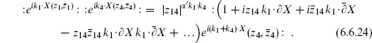
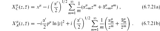
The Hilbert space expressions give us one more way to calculate expectations values. We take as an example the case of four exponential operators

We have used the result (2.7.11) that : : ordered operators are the same as ordered operators for this CFT. We have abbreviated X (z_i, _i) as and to avoid clutter are omitting the hats on operators. By definition

where

For |z₁| > |z₂| the matrix element (6.7.19) becomes

To evaluate this use the Campbell–Baker–Hausdorff (CBH) formula

The expectation value (6.7.22) becomes

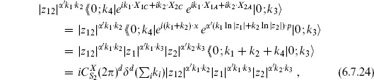
where we have used the two-point expectation value to normalize the last line. This is the familiar result (6.2.31), obtained by two other methods in section 6.2, after one includes in the latter a factor from the change of frame and takes z₄ → ∞. All other free-field results can be obtained by this same oscillator method.

Relation between inner products

Nondegenerate bilinear and Hermitean inner products can always be related to one another by an appropriate antilinear operation on the bra. Let us consider an example. From the free-field expectation values, we have

using the fact that |0;k maps to ^ik·X. Compare this with the inner product from the X CFT,

These differ only by k → −k from conjugating ^ik·X, and normalization,

For more general operators, there is a natural notion of conjugation in CFT. In Euclidean quantum mechanics, Hermitean conjugation inverts Euclidean time, eq. (A.1.37), so the natural operation of Euclidean conjugation is conjugation × time-reversal: an operator that is Hermitean in Minkowski space is also Hermitean under this combined operation. In CFT, we make the same definition, but also must include a time-reversal on the conformal frame,

Here p and p′ are related by radial time-reversal, z′ = ⁻¹, and the unprimed operator is in the z-frame and the primed operator in the u- frame. To see how this works, consider a holomorphic operator of weight h, whose Laurent expansion is

Its simple adjoint is

Then the Euclidean adjoint is

For an operator that is Hermitean in Minkowski time, , and so this operator is also Hermitean³ under . The Euclidean adjoint (6.7.28) conjugates all explicit factors of i, but leaves z and indices unchanged. This is its whole effect, other than an overall factor (−1)^{N_a(N_a − 1)/2} from reversing the order of anticommuting fields; here N_a is the total number of anticommuting fields in the operator.

This is the natural conformally invariant operation of conjugation, so it must be that

for some constant K. For a direct demonstration, the best we have come up with is

The only step here that is not either a definition or obvious is the assumption of proportionality, 1| = K 1|. This must hold because |1 is the unique SL(2, C)-invariant state.

For the X CFT we have seen that . For the ghost CFT, the Laurent expansion of the amplitude (6.3.4) gives 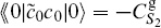, where |0 = ₁c₁|1. The Hermitean inner product was defined in eq. (4.3.18) as 0|₀c₀|0 = i, so .

Except for the is, which are absent in a unitary CFT, one can set K = 1 by adding an Euler number term to the action. In a Hermitean basis of operators, the two inner products are then identical, and the distinction between them is often ignored. Notice, however, that a vertex operator of definite nonzero momentum cannot be Hermitean.

Again, this can all be extended to the open string, with the disk in place of the sphere.

Exercises

6.1 Verify that the expectation value (6.2.31) is smooth in the u-patch.

6.2 For the linear dilaton CFT, Φ = VX, the X zero-mode path integral diverges. This reflects the fact that the coupling is diverging in some direction. Consider therefore imaginary Φ = ibX; this is unphysical but has technical applications (one could instead take complex momenta).
(a) Generalize the calculation that gave (6.2.17) to this case. Show that in the end the only changes are in the Weyl dependence (reflecting a change in the dimension of the exponential) and in the spacetime momentum conservation.
(b) Generalize the calculation of the same quantity using holomorphicity. Show that the result is the same as in the regular X CFT but with an extra background charge operator exp(−2ib · X) taken to infinity.

6.3 For one b and four c fields, show that expressions (6.3.5) and (6.3.8) are equal. Ignore the antiholomorphic fields.

6.4 (a) Write the amplitude for n open string tachyons on the disk as a generalization of eq. (6.4.5).
(b) Show by a change of variables that it is independent of the positions of the fixed vertex operators.

6.5 (a) Show that the residue of the pole in I(s, t) at ′ s = J − 1 is a polynomial in u − t of degree J, corresponding to intermediate particles of spin up to J.
(b) Consider the amplitude I(s, t) without assuming D = 26. In the center-of-mass frame, write the residue of the pole at ′s = 1 in terms of

where P⁰ projects onto spin 0 (the unit matrix) and P² projects onto spin 2 (traceless symmetric tensors). Show that the coefficient of P ⁰ is positive for D < 26, zero at D = 26, and negative at D > 26. Compare with the expected string spectrum at this level, and with the discussion of this level in section 4.1.

6.6 (a) In the hard scattering limit, evaluate the integral in the Veneziano amplitude (6.4.5) using the saddle point approximation. Take the naive saddle point; the justification requires consideration of the analytic continuations needed to define the integral.
(b) Do the same for the Virasoro–Shapiro amplitude.

6.7 (a) Derive the amplitude (6.5.12).
(b) Verify the relation (6.5.14) between vertex operator normalizations. Show that this agrees with the state–operator mapping.

6.8 Derive the three-gauge-boson amplitude (6.5.15).

6.9 (a) Obtain the four-gauge-boson amplitude. To reduce the rather extensive algebra, consider only those terms in which the polarizations appear as ₁ · _{2 3} · ₄.
(b) Compare the behavior at small ′k_i · k_j with the same amplitude in Yang–Mills theory.

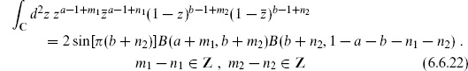
6.10 Carry out the integral in eq. (6.6.5) to obtain the Virasoro–Shapiro amplitude (6.6.10). The relation

is useful. (Reference: Green, Schwarz, & Witten (1987), section 7.2; note that their d²z is times ours.)

6.11 (a) Verify the amplitude (6.6.14).
(b) Verify the relation (6.6.15) between vertex operator normalizations.
(c) Complete the field theory calculation and verify the relation (6.6.18) between g_c and the gravitational coupling.

6.12 Calculate the disk amplitude with one closed string tachyon and two open string tachyons.

6.13 (a) Find the PSL(2, C) transformation that takes three given points z_1,2,3 into chosen positions _1,2,3.
(b) Verify the Möbius invariance results (6.7.3)–(6.7.7). Show that to derive (6.7.5) it is sufficient that L₁ and ₁ annihilate the operators.

6.14 (a) Find the PSL(2, R) transformation that takes three given points y_1,2,3 into chosen positions _1,2,3.
(b) Generalize the Möbius invariance results (6.7.3)–(6.7.7) to operators on the boundary of a disk.
(c) Find similar results for the disk with one interior, two interior, and one interior and one boundary operators.

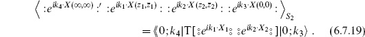
6.15 (a) Generalize the operator calculation (6.7.24) to a product of n exponentials.
(b) Generalize it to the expectation value (6.2.25).

__________

¹  A curious factor of i has been inserted into eq. (6.2.6) by hand because it is needed in the S-matrix, but it can be understood formally as arising from the same rotation. If we rotated the entire field X⁰ → − iX ^d, the Jacobian should be 1, by the usual argument about rescaling fields (footnote 1 of the appendix). However, we do not want to rotate , because this mode produces the energy delta function. So we have to rotate it back, giving a factor of i.

²  The constant also depends on the conformal factor, because the X CFT by itself has nonzero central charge, but in the full string theory this will cancel.

³  Because its Laurent expansion has no factor of i, the Faddeev–Popov c ghost is actually anti-Hermitean under the Euclidean adjoint. This is due to an inconvenient conflict between conventions, and has no significance.