7

One-loop amplitudes

After describing the relevant surfaces, we focus on the torus, first on the CFTs on this surface and then on the string amplitudes. We then generalize to the open and unoriented theories. The most important issue to be understood is the absence of short-distance (UV) divergences.

7.1    Riemann surfaces

There are four Riemann surfaces with Euler number zero.

The torus

The torus T², discussed in section 5.1, is the only closed oriented surface with Euler number zero. We describe it as the complex plane with metric and identifications

There are two moduli, the real and imaginary parts of , and two CKVs, the translations. In terms of the real coordinates w = ¹ + i²,

so that one can think of the torus as a cylinder of circumference 2 and length 2₂ with the ends rotated by an angle of 2₁ and then sewn together.

In terms of the coordinate z = exp(−iw), the identification is automatic, while becomes

A fundamental region is the annulus

The torus is formed by rotating the outer circle by 2₁ and then sewing the inner and outer circles together. We will use the w-coordinate unless otherwise noted.

The cylinder (annulus)

The cylinder C₂ is the region

That is, it is a strip of width and length 2t, with the ends joined. There is a single modulus t, which runs over the whole range 0 < t < ∞. Unlike the torus there is no modular group, the long-cylinder limit t → 0 being quite different from the long-strip limit t → ∞. There is a single CKV, the translation parallel to the boundary.

The cylinder can be obtained from the torus with imaginary = it by identifying under the involution

which is a reflection through the imaginary axis. The lines ¹ = 0, are fixed by this reflection and so become boundaries. The other coordinate is periodically identified,

The Klein bottle

The Klein bottle K₂ can be regarded as the complex plane with identification

or

This is a cylinder of circumference 2 and length 2t, with the ends sewn together after a parity-reversal Ω. The single modulus t runs over 0 < t < ∞, and there is no modular group. Translation in the ² direction is the only CKV. The Klein bottle can be obtained from the torus with modulus = 2it by identifying under

The Klein bottle can be thought of as a sphere with two cross-caps, but we postpone this description until section 7.4.

The Möbius strip

The Möbius strip M₂ is sewn from a strip with a twist by Ω,

Again the modulus t runs over 0 < t < ∞ and the only CKV is the ²- translation. It can be obtained from the torus with = 2it by identifying under the two involutions

The Möbius strip can be thought of as a disk with a cross-cap, but again we defer this description.

7.2    CFT on the torus

Scalar correlators

As in the case of the sphere, we start with the Green’s function (6.2.7), satisfying

The Green’s function is periodic in both directions on the torus, and aside from the source and the background charge term it would be the sum of holomorphic and antiholomorphic functions. These properties identify it as being associated with the theta functions, whose properties are given at the end of this section. In particular we guess

The function ₁ vanishes linearly when its first argument goes to zero, giving the correct behavior as w → w′. Elsewhere the logarithm is the sum of holomorphic and antiholomorphic functions and so is annihilated by . However, this function is not quite doubly periodic owing to the quasiperiodicity (7.2.32b) — it changes by under w → w + 2. Also, the background charge is missing. Both properties are easily corrected:

The function k(, ) is determined by orthogonality to ₀, but as in the case of the sphere it drops out due to spacetime momentum conservation.

The expectation value of a product of vertex operators is given, in parallel to the earlier result (6.2.13) on the sphere, by

The factor comes from the renormalized self-contractions.

The scalar partition function

The overall normalization of the sphere was absorbed into the string coupling constant, but we cannot do this for the torus, in particular because there is a nontrivial -dependence. In fact, we will see that there is a great deal of physics in the amplitude with no vertex operators at all. Consider the path integral with no vertex operators, 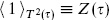. We can think of the torus with modulus as formed by taking a field theory on a circle, evolving for Euclidean time 2₂, translating in ¹ by 2₁, and then identifying the ends. In operator language this gives a trace,

Here q = exp(2i), the momentum P = L₀ − ₀ generates translations of ¹, and the Hamiltonian generates translations of ² as in eq. (2.6.10). Such a trace, weighted by the exponential of the Hamiltonian and other conserved quantities, is termed a partition function as in statistical mechanics.

The trace breaks up into a sum over occupation numbers N_n and _n for each and n and an integral over momentum k. The Virasoro generators similarly break up into a sum, and Z () becomes

The factor of spacetime volume V_d comes from the continuum normalization of the momentum, becoming . The various sums are geometric,

and so we obtain

where

Here

is the Dedekind eta function, discussed further at the end of the section. The i comes from the rotation k⁰ → ik^d needed to define the divergent integral. Also, the earlier is Z_X ()^d.

The result (7.2.8) is obviously invariant under → + 1. Invariance of Z_X under → − 1/ follows from eq. (7.2.44), , thus generating the full modular group. Similarly the expectation value with vertex operators is modular-covariant, taking into account the Weyl transformations of the operators.

We have evaluated the path integral by translating into an operator expression, but as on the sphere there are two other methods. We leave to the reader the direct path integral evaluation. Fourier transforming in ¹, it just breaks up into a product of harmonic oscillator path integrals.

The evaluation using holomorphicity is less direct. We include it for illustration because it is used at higher genus and for more complicated CFTs. The idea is to get a differential equation with respect to . Consider the torus with modulus and make a small change in the metric, . The new metric is

That is, the metric is Weyl-equivalent to dw′ d′ with . This has the periodicities

This change in the metric is therefore equivalent to a change

in the modulus.

Under a change in the metric, the change in the path integral is

In the second line we have used translation invariance to carry out the integral over w. All expectation values are understood to be on the torus with modulus . To get the expectation value of the energy-momentum tensor, we use the OPE

Now,

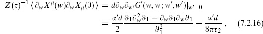
where the arguments of all the theta functions are (w/2, ). This does indeed have a double pole at w = 0. Carefully expanding both numerator and denominator to order w² (this is simplified by the fact that ₁ is odd), the order w⁰ term in the expectation value (7.2.16) is

The OPE (7.2.15) then gives

and the variation (7.2.14) gives the differential equation

To proceed further, we use the fact, which is easily verified from the infinite sum, that the theta functions satisfy

Rewrite (7.2.19) as

Together with the conjugate equation, this determines

up to a numerical coefficient that must be fixed by other means. Noting the relation (7.2.43), this is the same as the earlier result (7.2.8).

The bc CFT

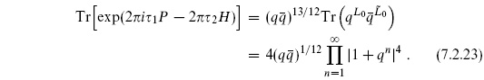
For the ghost CFT, the partition function is again determined easily in terms of a trace over states. There are two sets of raising operators b_−n and c_−n on both the right and left, but now these are anticommuting so the occupation numbers can only be zero or one — a single oscillator at mode n thus gives (1+qⁿ). In addition there are four ground states, giving

Recall, however, that for anticommuting fields the simple trace corresponds to a path integral with antiperiodic boundary conditions in the time direction. In order to calculate the Faddeev–Popov determinant, the ghosts must have the same periodicity as the original coordinate transformations, which were periodic. Thus we need

where (−1)^F anticommutes with all the ghost fields. The trace vanishes because the states and have opposite ghost number mod 2 from and . From the path integral point of view, Z () vanishes due to ghost zero modes from the moduli and CKVs. These must be saturated with appropriate insertions, the simplest nonvanishing amplitude (and the one we will need) being

In the operator calculation we write each field in terms of its mode expansion. Only the n = 0 terms contribute, the expectation values of the others vanishing as above. Then (7.2.25) becomes

The operator projects onto the single ground state , so the result is

Note the sign change in the infinite product, from the (−1)^F in the trace. The result (7.2.27) is independent of the positions of the ghost fields because the CKV and quadratic differentials on the torus are constants. Again, we do not try to keep track of the overall sign, setting it to be positive.

General CFTs

For general CFTs,

where i runs over all states of the CFT, and F_i is again the world-sheet fermion number. Invariance under → + 1 requires 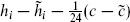to be a to be an integer. Looking at the unit operator, this requires c − to be a multiple of 24. For general operators one then has the requirement that the spin be an integer,

Incidentally, CFTs for which c − is not a multiple of 24 are certainly of interest. These cannot be separately modular-invariant, but with appropriate projections can be combined into a modular-invariant theory.

Invariance under → −1/ puts a further constraint on the spectrum. Let us here note just one general consequence, which relates the states of large h to those of lowest h. Consider the partition function for = i as → 0. The convergence factor q = exp(−2) is approaching unity, so the partition function is determined by the density of states at high weight. Using modular invariance, this is equal to the partition function at = i/. In the latter case, q = exp(−2/) is going to zero, so the state of lowest weight dominates the sum. This is the unit state, with L₀ = ₀ = 0, giving

The density of states at high weight is thus determined by the central charge. This generalizes the free-boson result, where c = = d counts the number of free bosons.¹

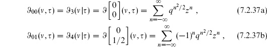
Theta functions

The basic theta function is

It has the periodicity properties

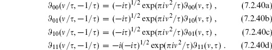
and these in fact determine it up to normalization. Under modular transformations,

The theta function has a unique zero, up to the periodicity (7.2.32), at . It can also be written as an infinite product,

in terms of

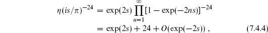
We often need the asymptotic behavior of the theta function as q → 0 or as q → 1. The q → 0 behavior can be read immediately from either the infinite sum or infinite product form. The q → 1 behavior is not manifest in either form, because an infinite number of terms contribute. It can be obtained from the → −1/ modular transformation, which relates these two limits by q → exp(4²/ ln q).

It is also useful to define the theta function with characteristics,

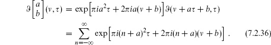
Other common notations are

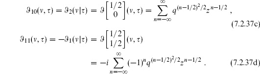
These have the product representations

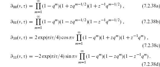
Their modular transformations are

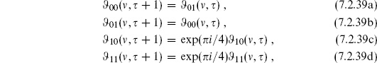
and

We will encounter these functions more extensively in the superstring.

The theta function satisfies Jacobi’s ‘abstruse identity,’ a special case of a quartic identity of Riemann,

Note also that

Finally, the Dedekind eta function is

It has the modular transformations

7.3    The torus amplitude

We now apply to the torus the general result (5.3.9) expressing the string amplitude as an integral with ghost and vertex operator insertions. The two CKVs require one vertex operator to be fixed, so

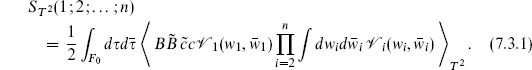
The fundamental region F₀ and the factor of from w → −w were discussed in section 5.1. As usual for complex variables, 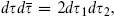where The ghost insertion for d is

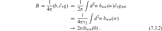
We have used the result (7.2.13) for the -derivative of the metric. In the final line we have used the fact that the ghost path integral (7.2.27) is independent of position to carry out the w-integration. (Recall that and that g_w = .)

The CKG consists of the translations of the torus. Since this group has finite volume, we need not fix it: we can rewrite the amplitude so that all vertex operators are integrated and the volume of the CKG is divided out. It is easy to do this by hand here. The CKVs are constant, so the expectation value in eq. (7.3.1) is independent of where the c ghosts are placed: we can move them away from w₁, putting them at some fixed position. For the vertex operators, translation invariance implies that the amplitude is unchanged if we replace w_i → w_i + w. Average over translations

the denominator being the area of the torus, which is the volume of the CKG. Using eqs. (7.3.2) and (7.3.3), the amplitude becomes

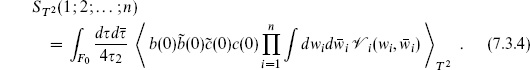
All vertex operators are now on an equal footing.

The form (7.3.4) could also have been derived directly, without the intermediate step of fixing a vertex operator, and is valid even without vertex operators,

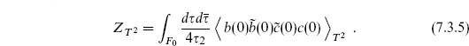
This vacuum amplitude is quite interesting and will be our main focus. Not only does it reveal the essential difference between the ultraviolet behaviors of string theory and field theory, but it has an important physical interpretation of its own.

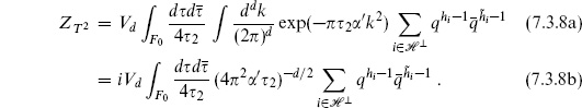
For 26 flat dimensions, the matter and ghost path integrals (7.3.5) were evaluated in the previous section, with the result

The amplitude has the important property of modular invariance. The product is invariant by eq. (7.2.44), and it is easy to check that

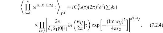
is modular-invariant as well. Note the exponent −48, from the 24 left-and right-moving oscillators. The contribution of the ghosts cancels two sets of oscillators, leaving only the contribution of the transverse modes. The amplitude with n tachyons is given by including the vertex operator expectation value (7.2.4) and integrating over positions.

For a general CFT the path integral on the torus is expressed as a trace in eq. (7.2.28). As long as there are d ≥ 2 noncompact flat dimensions the ghosts still cancel two sets of bosonic operators, and the vacuum amplitude is

Here is the closed string Hilbert space excluding the ghosts, the = 0, 1 oscillators, and the noncompact momenta.

In order to understand the physics of these amplitudes it is useful to compare with the corresponding quantity in field theory, the sum over all particle paths with the topology of a circle. This is given by

This can be derived by gauge-fixing the point-particle path integral, which was given as exercise 5.2. The result is intuitive: l is the modulus for the circle, (k² + m²) is the world-line Hamiltonian, and the 2l in the denominator removes the overcounting from translation and reversal of the world-line coordinate.

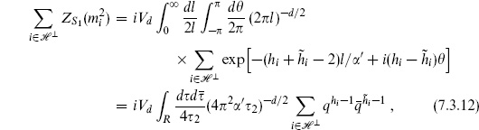
Let us now take this point-particle result, which is for a particle of given m², and sum over the actual spectrum of the string. As shown in chapter 4, the physical spectrum is in one-to-one correspondence with , where the mass is related to the transverse weights by

and with the constraint It is useful to write the latter constraint in integral form,

In writing this we are assuming that the difference is an integer. This is true in 26 flat dimensions, and as we have discussed in the previous section it is necessary in general for modular invariance. Then

where Here the region of integration R is

Now let us interpret these results. The amplitude (7.3.9) for a single point particle diverges as l → 0. This is the usual UV divergence of quantum field theory (note that l has units of spacetime length-squared). Summing this over the string spectrum as in eq. (7.3.12) only makes things worse, as all the states of the string contribute with the same sign. However, compare the sum (7.3.12) to the actual string amplitude (7.3.8). There is great similarity but also one remarkable difference. The integrands are identical but the regions of integration are different: in the string it is the fundamental region

and in field theory the larger region R. In the string amplitude, the UV divergent region is simply absent. We can also see this from the point of view of the momentum integral (7.3.8a). Since ₂ is bounded below, this integral (after contour rotation) is a convergent Gaussian.

Another possible divergence comes from the limit ₂ → ∞, where the torus becomes very long. In this region, the string amplitude in 26 flat dimensions has the expansion

the asymptotic behavior being controlled by the lightest string states. The first term in the series diverges, and the interpretation is clear from the field theory point of view. The series is in order of increasing mass-squared. The first term is from the tachyon and diverges due to the positive exponential in the path sum (7.3.9). This divergence is therefore an artifact of a theory with a tachyon, and will not afflict more realistic string theories. Incidentally, this path sum can be defined by analytic continuation from positive mass-squared, but there is still a pathology — the continued energy density is complex. This signifies an instability, the tachyon field rolling down its inverted potential. With a general CFT, eq. (7.3.12) becomes

Because the tachyon is always present in bosonic string theory this again diverges; in the absence of tachyons it will converge.

The torus illustrates a general principle, which holds for all string amplitudes: there is no UV region of moduli space that might give rise to high energy divergences. All limits are controlled by the lightest states, the long-distance physics. For the torus with vertex operators the -integration is still cut off as above, but there are more limits to consider as vertex operators approach one another. The same general principle applies to these as well, as we will develop further in chapter 9.

One might try to remove the UV divergence from field theory by cutting off the l integral. Similarly, one might try to make an analogous modification of string theory, for example replacing the usual fundamental region F₀ with the region whose lower edge is straight. However, in either case this would spoil the consistency of the theory: unphysical negative norm states would no longer decouple. We have seen in the general discussion in section 5.4 that the coupling of a BRST-null state is proportional to a total derivative on moduli space. For the fundamental region F₀, the apparent boundaries I and I′ and II and II′ respectively (shown in fig. 5.2) are identified and the surface terms cancel. Modifying the region of integration introduces real boundaries. Surface terms on the modified moduli space will no longer cancel, so there is nonzero amplitude for null states and an inconsistent quantum theory. This is directly analogous to what happens in gravity if we try to make the theory finite by some brute force cutoff on the short-distance physics: it is exceedingly diffcult to do this without spoiling the local spacetime symmetry and making the theory inconsistent. String theory manages in a subtle way to soften the short-distance behavior and eliminate the divergences without loss of spacetime gauge invariance.

Physics of the vacuum amplitude

Besides serving as a simple illustration of the behavior of string amplitudes, the one-loop vacuum amplitude has an interesting physical interpretation. In point-particle theory, ‘vacuum’ paths consist of any number n of disconnected circles. Including a factor of 1/n! for permutation symmetry and summing in n leads to

Translating into canonical field theory,

where ₀ is the vacuum energy density:

The l integral in diverges as l → 0. In renormalizable field theory this divergence is canceled by counterterms or supersymmetry. To get a rough insight into the physics we will cut off the integral at l ≥ and then take → 0, but drop divergent terms. With this prescription,

and

where . Using the latter form, the vacuum energy density becomes

which is just the sum of the zero-point energies of the modes of the field. This is in spacetime, of course — we encountered the same kind of sum but on the world-sheet in section 1.3.

The description of a quantum field theory as a sum over particle paths is not as familiar as the description in terms of a sum over field histories, but it is equivalent. In particular, the free path integral in field theory can be found in most modern field theory textbooks:

Using eq. (7.3.20), this is the same as the path sum result (7.3.9).

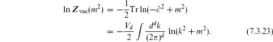
In older quantum field theory texts, one often reads that vacuum amplitudes such as eq. (7.3.18) are irrelevant because they give an overall phase that divides out of any expectation value. This is true if one is considering scattering experiments in a fixed background and ignoring gravity, but there are at least two circumstances in which the vacuum energy density is quite important. The first is in comparing the energy densities of different states to determine which is the true ground state of a theory. It is very likely, for example, that the breaking of the electroweak SU (2) × U (1) symmetry is determined in part by such quantum corrections to the vacuum energy density. This was the original motivation that led to the Coleman–Weinberg formula (7.3.23). The generalization to a theory with particles of arbitrary spin is

The sum runs over all physical particle states. Each polarization counts separately, giving a factor of for a particle of spin s_i in four dimensions. Here F_i is the spacetime fermion number, defined mod 2, so fermions contribute with the opposite sign.

The second circumstance is when one considers the coupling to gravity. The vacuum energy gives a source term in Einstein’s equation, the cosmological constant, and so has observable effects. In fact, this cosmological constant is a great challenge, because the fact that spacetime is approximately flat and static means that its value is very small,

If one considers only the contributions to the vacuum energy from the vacuum fluctuations of the known particles up to the currently explored energy (roughly the electroweak scale m_ew), the zero-point energy is already of order

52 orders of magnitude too large. The Higgs field potential energy and the QCD vacuum energy are also far too large. Finding a mechanism that would account for the cancellation of the net cosmological constant to great accuracy has proven very difficult. For example, in a supersym-metric theory, the contributions of degenerate fermions and bosons in the sum (7.3.24) cancel. But supersymmetry is not seen in nature, so it must be a broken symmetry. The cancellation is then imperfect, leaving again a remainder of at least . The cosmological constant problem is one of the most nagging diffculties, and therefore probably one of the best clues, in trying to find a unified theory with gravity.

What about the cosmological constant problem in string theory? At string tree level we had a consistent theory with a flat metric, so the cosmological constant was zero. In fact we arranged this by hand, when we took 26 dimensions. One sees from the spacetime action (3.7.20) that there would otherwise be a tree-level potential energy proportional to D − 26. The one-loop vacuum energy density in bosonic string theory is nonzero, and is necessarily of the order of the string scale (ignoring the tachyon divergence). In four dimensions this would correspond to 10⁷² GeV⁴, which is again far too large. In a supersymmetric string theory, there will be a certain amount of cancellation, but again one expects a remainder of at least in a realistic theory with supersymmetry breaking.

The cosmological constant problem is telling us that there is something that we still do not understand about the vacuum, in field theory and string theory equally. We will return to this problem at various points.

7.4    Open and unoriented one-loop graphs

The cylinder

The results for the torus are readily extended to the other surfaces of Euler number zero. For example, the vacuum amplitude from the cylinder in the oriented theory is

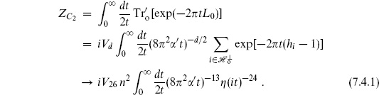
This can be obtained either by working out the path integral measure in terms of the ghost zero modes, as we did for the torus, or by guessing (correctly) that we should again sum the point-particle result (7.3.9) over the open string spectrum. In the first line, the trace is over the full open string CFT, except that for omission of the ghost zero modes as denoted by the prime. In the final line the trace has been carried out for the case of 26 flat dimensions, with n Chan–Paton degrees of freedom. Including tachyon vertex operators is straightforward.

The t → ∞ limit of the cylinder is much like the ₂ → ∞ limit of the torus. The cylinder looks like a long strip, and the leading asymptotics are given by the lightest open string states. As in the closed string there is a divergence, but only from the open string tachyon.

The t → 0 limit is rather interesting. Unlike the case of the torus, there is no modular group acting to cut off the range of integration, and so the UV divergence of field theory still seems to be present. However, we will see that, as with all divergences in string theory, this should actually be interpreted as a long-distance effect. In the t → 0 limit the cylinder is very long as shown in figure 7.1(a). That is, it looks like a closed string appearing from the vacuum, propagating a distance, and then disappearing again into the vacuum. To make this clear, use the modular transformation (7.2.44)

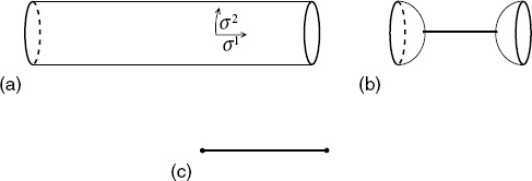
Fig. 7.1.   (a) Cylinder in the limit of small t. (b) The amplitude separated into disk tadpole amplitudes and a closed string propagator. (c) Analogous field theory graph. The heavy circles represent the tadpoles.

and change variables to s = /t, with the result

Scaling down the metric by 1/t so that the cylinder has the usual closed string circumference 2, the length of the cylinder is s. Expanding

one sees the expected asymptotics from expanding in a complete set of closed string states. In other words, if we think of ² as world-sheet time and ¹ as world-sheet space, figure 7.1(a) is a very short open string loop. If we reverse the roles of world-sheet space and time, it is a very long closed string world-line beginning and ending on boundary loops. In the Euclidean path integral, either description can be used, and each is useful in a different limit of moduli space.

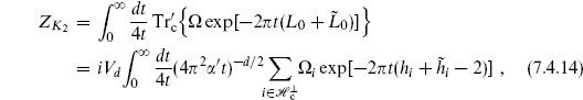
The leading divergence in the vacuum amplitude is from the closed string tachyon. This is uninteresting and can be defined by analytic continuation,

The second term, from the massless closed string states, gives a divergence of the form 1/0 even with the continuation. To see the origin of this divergence, imagine separating the process as shown in figure 7.1(b). As we have discussed in section 6.6, there is a nonzero amplitude with one closed string vertex operator on the disk. This tadpole corresponds to a closed string appearing from or disappearing into the vacuum. In between the two tadpoles is the closed string propagator. In momentum space the massless propagator is proportional to 1/k². Here, momentum conservation requires that the closed string appear from the vacuum with zero momentum, so the propagator diverges.

This same kind of divergence occurs in quantum field theory. Consider a massless scalar field with a term linear in in the Lagrangian. There is then a vertex which connects to just a single propagator, and the graph shown in figure 7.1(c) exists. This diverges because the intermediate propagator is

This is a long-distance (IR) divergence, because poles in propagators are associated with propagation over long spacetime distances.

UV and IR divergences in quantum field theory have very different physical origins. UV divergences usually signify a breakdown of the theory, the need for new physics at some short distance. IR divergences generally mean that we have asked the wrong question, or expanded in the wrong way. So it is here. In normal perturbation theory we expand around () = 0, or some other constant configuration. For the action

the equation of motion

does not allow () = 0 as a solution. Instead we must expand around a solution to the equation (7.4.8); any solution is necessarily position-dependent. The resulting amplitudes are free of divergences. This is true even though the right-hand side is a perturbation (we have included the factor of g appropriate to the disk), because it is a singular perturbation. In particular, the corrected background breaks some of the Poincaré symmetry of the zeroth order solution.

The situation is just the same in string theory. The disk tadpole is a source

for both the dilaton and metric. Expanding around a solution to the corrected field equations (with the metric and dilaton no longer constant) leads to finite amplitudes. The details are a bit intricate, and will be discussed somewhat further in chapter 9. Incidentally, in supersymmetric string theories if the tree-level background is invariant under supersymmetry, it usually receives no loop corrections.

The pole (7.4.6) is the same kind of divergence encountered in the tree-level amplitudes, a resonance corresponding to propagation over long spacetime distances. If we add open string vertex operators to each end of the cylinder so that it represents a one-loop open string scattering amplitude, then the momentum k flowing from one boundary to the other is in general nonzero. The large-s limit (7.4.4) then includes a factor of

and the divergence becomes a momentum pole representing scattering of open strings into an intermediate closed string. Thus, as claimed in chapter 3, an open string theory must include closed strings as well. It is curious that the mechanism that removes the UV divergence is different in the closed and open string cases. In the closed string it is an effective cutoff on the modular integration; in the open string it is a reinterpretation of the dangerous limit of moduli space in terms of long distances.

In eq. (7.4.1) the path integral on the cylinder has been related to a trace over the open string spectrum by cutting open the path integral with ² treated as time. It can also be obtained in terms of the closed string Hilbert space by treating ¹ as time. Let ² be periodic with period 2 and the boundaries be at ¹ = 0, s. The closed string appears in some state |B at ¹ = 0 and then disappears in the same way at ¹ = s. Including the measure insertions, the path integral is then proportional to

The boundary state |B is determined by the condition that ₁X, c¹, and b₁₂ vanish on the boundary. In the Hamiltonian form these must annihilate |B , which in terms of the Laurent coeffcients is

This determines

Using this in (7.4.11) gives the result (7.4.3), except that the normalization of |B is undetermined. This representation is useful in analyzing the t → 0 limit and the closed string poles.

By comparing the string and field theory calculations we can determine the disk tadpole Λ, but it will be more convenient to do this in the next chapter as a special case of a more general result.

The Klein bottle

The vacuum amplitude from the Klein bottle is

where the notation follows the cylinder (7.4.1). Relative to the torus in the oriented theory there is an extra factor of from the projection operator (1 + Ω). For the same reason there is an extra in both the torus and cylinder amplitudes in the unoriented theory. One can also think of this as coming from the extra gauge invariance w → . To evaluate the trace for 26 flat dimensions, note that the only diagonal elements of Ω are those for which the right- and left-movers are in the same state, and these states contribute with Ω = +1. The trace is then effectively over only one side, which is the same as the open string spectrum, except that the weight is doubled because the right- and left-movers make equal contributions. The result is

The modulus t runs over the same range 0 < t < ∞ as for the cylinder, so the t → 0 divergences are the same. Again the 1/0 pole has a long-distance interpretation in terms of a closed string pole. To see this consider the regions

each of which is a fundamental region for the identification

In (7.4.16a), the left- and right-hand edges are periodically identified while the upper and lower edges are identified after a parity-reversal, giving an interpretation as a closed string loop weighted by Ω. For (7.4.16b), note that the identifications (7.4.17) imply also that

It follows that the upper and lower edges of the region (7.4.16b) are periodically identified. The left-hand edge is identified with itself after translation by half its length and reflection through the edge, and similarly the right-hand edge: this is the definition of a cross-cap. Thus we have the representation in figure 7.2(a) as a cylinder capped by two cross-caps. Rescaling by 1/2t, the cylinder has circumference 2 and length s = /2t. After a modular transformation, the amplitude becomes

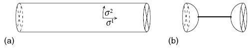
Fig. 7.2.   (a) Klein bottle in the limit of small t as a cylinder capped by cross-caps. (b) The amplitude separated into RP₂ tadpole amplitudes and a closed string propagator.

All the discussion of the cylinder divergence now applies, except that the tadpole is from the projective plane rather than the disk.

The Möbius strip

For the Möbius strip,

This differs from the result on the cylinder only by the Ω and the factor of from the projection operator. In 26 flat dimensions, the effect of the operator Ω in the trace is an extra −1 at the even mass levels plus an appropriate accounting of the Chan–Paton factors. The oscillator trace is thus

For the SO(n) theory the n(n + 1) symmetric states have Ω = +1 while the n(n − 1) antisymmetric states have Ω = −1 for a net contribution of n. For the Sp(k) theory these degeneracies are reversed, giving −n (recall that in our notation Sp(k) corresponds to n = 2k Chan–Paton states). The amplitude is then

By the same construction as for the Klein bottle, the Möbius strip can be represented as a cylinder with a boundary at one end and a cross-cap on the other, as in figure 7.3(a). The length of the cylinder is now s = /4t. By a modular transformation, the amplitude becomes

Fig. 7.3.   (a) Möbius in the limit of small t as a cylinder capped by one cross-cap. (b) The amplitude separated into D₂ and RP₂ tadpole amplitudes and a closed string propagator.

As for the annulus this can be written as an operator expression, one of the boundary states in eq. (7.4.11) being replaced by an analogous cross-cap state |C . There is again a t → 0 divergence; it corresponds to the process of figure 7.3(a) with one tadpole from the disk and one from the projective plane.

In the unoriented theory the divergences on these three surfaces combine into

That is, the total tadpole is proportional to 2¹³ n. For the gauge group SO(2¹³) = SO(8192) this vanishes, the tadpoles from the disk and projective plane canceling. For the bosonic string this probably has no special significance, but the analogous cancellation for SO(32) in superstring theory does.

Exercises

7.1 Fill in the steps leading to the expectation value (7.2.4) of exponential operators on the torus. Show that it has the correct transformation under → −1/.

7.2 Derive the torus vacuum amplitude (7.3.6) by regulating and evaluating the determinants, as is done for the harmonic operator in appendix A. Show that a modular transformation just permutes the eigenvalues. [Compare exercise A.3.] (Reference: Polchinski (1986).)

7.3 Derive the Green’s function (7.2.3) by carrying out the eigenfunction sum (6.2.7).

7.4 Evaluate on the torus by representing it as a trace. Show that the result agrees with eq. (7.2.16).

7.5 (a) Obtain the leading behavior of the theta functions (7.2.37) as Im → ∞.
(b) By using the modular transformations, do the same as → 0 along the imaginary axis.
(c) A more exotic question: what if approaches a nonzero point on the real axis, along a path parallel to the imaginary axis? [Hint: the answer depends crucially on whether the point is rational or irrational.]

7.6 (a) Verify eqs. (7.3.20) and (7.3.21).
(b) Evaluate Z_S1(m²) with a cutoff on the l-integral in any dimension d. Show that the counterterms are analytic in m². Give the nonanalytic part for d = 4. (Reference: Coleman & Weinberg (1973).)

7.7 Obtain the amplitude for n open string tachyons on the cylinder in a form analogous to the torus amplitude (eq. (7.3.6) combined with eq. (7.2.4)). The necessary Green’s function can be obtained from that on the torus by the method of images, using the representation of the cylinder as an involution of the torus.

7.8 Consider the amplitude from the previous problem, in the case that there are some vertex operators on each of the two boundaries. Show from the explicit result of the previous problem that the t → 0 limit gives a series of closed string poles as a function of the momentum flowing from one boundary to the other.

7.9 If you have done both exercises 6.12 and 7.8, argue that unitarity relates the square of the former to the tachyon pole of the latter. Use this to find the numerical relation between g_c and . We will do something similar to this, in a more roundabout way, in the next chapter.

7.10 Argue that unitarity of the cylinder amplitude with respect to intermediate open strings requires the Chan–Paton factors to satisfy

Show that the gauge group U(n₁) × U(n₂) × … × U(n_k) is consistent with unitarity at tree level, but that this additional condition singles out U(n).

7.11 This exercise reproduces the first appearance of D = 26 in string theory (Lovelace, 1971). Calculate the cylinder vacuum amplitude from the Coleman–Weinberg formula in the form (7.3.9), assuming D spacetime dimensions and D′ net sets of oscillators. Fix the constant in the open string mass-squared so that the tachyon remains at m² = −1/′, as required by conformal invariance of the vertex operator. Insert an additional factor of exp(−′k²s / 2) as in eq. (7.4.10) to simulate a scattering amplitude. Show that unless D = 26 and D′ = 24, the amplitude has branch cuts (rather than poles) in k².

7.12 Repeat the previous exercise for the torus, showing in this case that the vacuum amplitude is modular-invariant only for D = 26 and D′ = 24 (Shapiro, 1972).

7.13 Carry out the steps, parallel to those used to derive the torus amplitude (7.3.6), to obtain the vacuum Klein bottle amplitude (7.4.15) from the string path integral.

7.14 Show that the amplitude (7.4.11) with the boundary state (7.4.13) reproduces the cylinder amplitude (7.4.3).

7.15 (a) Find the state |C corresponding to a cross-cap.
(b) By formulae analogous to eq. (7.4.11), obtain the Klein bottle and Möbius strip vacuum amplitudes.

__________

¹  To be precise, the result (7.2.30) holds in compact unitary CFTs. In nonunitary theories there are usually operators of negative weight, whose contribution will dominate that of the unit operator. In the linear dilaton theory, the central charge depends on V but the density of states does not: here the exception occurs because of complications due to the noncompactness of X combined with lack of translation invariance.