6
Matrix Computing

This chapter examines various aspects of computing with matrices, and in particular applications of the Python packages. Because these packages are optimized and robust, we strongly recommend their use even in all your small programs (small programs often grow big). The two-mass-on-a-string problem is formulated as a matrix problem, and extends the Newton–Raphson search technique to be discussed in Chapter 7. Although there is some logic in having this chapter after Chapter 7, it is placed here to provide the matrix tools needed for visualizations (which is why Problem 3 preceds 1).

6.1 Problem 3: N–D Newton–Raphson; Two Masses on a String

Problem Two weights (W₁, W₂) = (10, 20) are hung from three pieces of string with lengths (L₁, L₂, L₃) = (3, 4, 4) and a horizontal bar of length L = 8 (Figure 6.1). Find the angles assumed by the strings and the tensions exerted by the strings.

In spite of the fact that this is a simple problem requiring no more than first-year physics to formulate, the coupled transcendental equations that result are just about inhumanely painful to solve analytically.¹⁾ However, we will show you how the computer can solve this problem, but even then only by a trial-and-error technique with no guarantee of success. Your problem is to test this solution for a variety of weights and lengths and then to extend it to the three-weight problem (not as easy as it may seem). In either case check the physical reasonableness of your solution; the deduced tensions should be positive and similar in magnitude to the weights of the spheres, and the deduced angles should correspond to a physically realizable geometry, as confirmed with a sketch such as Figure 6.2. Some of the exploration you should do is to see at what point your initial guess gets so bad that the computer is unable to find a physical solution.

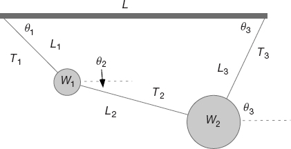
Figure 6.1 Two weights connected by three pieces of string and suspended from a horizontal bar of length L. The lengths are all known, but the angles and the tensions in the strings are to be determined.

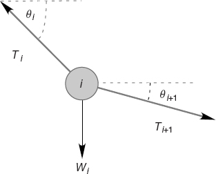
Figure 6.2 A free body diagram for one weight in equilibrium. Balancing the forces in the x and y directions for all weights leads to the equations of static equilibrium.

6.1.1 Theory: Statics

We start with the geometric constraints that the horizontal length of the structure is L and that the strings begin and end at the same height (Figure 6.1):

(6.1)

(6.2)

(6.3)

(6.4)

(6.5)

Observe that the last three equations include trigonometric identities as independent equations because we are treating sin θ and cos θ as independent variables; this makes the search procedure easier to implement. The basics physics says that because there are no accelerations, the sum of the forces in the horizontal and vertical directions must equal zero (Figure 6.2):

(6.6)

(6.7)

(6.8)

(6.9)

Here W_i is the weight of mass i and T_i is the tension in string i. Note that because we do not have a rigid structure, we cannot assume the equilibrium of torques.

6.1.2 Algorithm: Multidimensional Searching

Equations (6.1)–(6.9) are nine simultaneous nonlinear equations. While linear equations can be solved directly, nonlinear equations cannot (Press et al., 1994). You can use the computer to search for a solution by guessing, but there is no guarantee of finding one.

Unfortunately, not everything in life is logical, as we need to use a search technique now that will not be covered until Chapter 7. While what we do next is self-explanatory, you may want to look at Chapter 7 now if you are not at all familiar with searching.

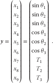
We apply to our set the same Newton–Raphson algorithm as used to solve a single equation by renaming the nine unknown angles and tensions as the subscripted variable y_i and placing the variables together as a vector:

(6.10)

The nine equations to be solved are written in a general form with zeros on the right-hand sides and placed in a vector:

(6.11)

(6.12)

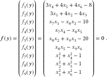
The solution to these equations requires a set of nine x_i values that make all nine f_i’s vanish simultaneously. Although these equations are not very complicated (the physics after all is elementary), the terms quadratic in x make them nonlinear, and this makes it hard or impossible to find an analytic solution. The search algorithm guesses a solution, expands the nonlinear equations into linear form, solves the resulting linear equations, and continues to improve the guesses based on how close the previous one was to making f = 0. (We discuss search algorithms using this procedure in Chapter 7.)

Explicitly, let the approximate solution at any one stage be the set x_i and let us assume that there is an (unknown) set of corrections Δx_i for which

(6.13)

We solve for the approximate Δx_i’s by assuming that our previous solution is close enough to the actual one for two terms in the Taylor series to be accurate:

(6.14)

We now have a solvable set of nine linear equations in the nine unknowns Δx_i, which we express as a single matrix equation

(6.15)

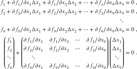
Note now that the derivatives and the f’s are all evaluated at known values of the x_i’s, so that only the vector of the Δx_i values is unknown. We write this equation in matrix notation as

(6.16)

Here we use bold italic letters to emphasize the vector nature of the columns of f_i and Δx_i values, and denote the matrix of the derivatives F′ (it is also sometimes denoted by J because it is the Jacobian matrix).

The equation F′ Δx = − f is in the standard form for the solution of a linear equation (often written as Ax = b), where Δx is the vector of unknowns and b = − f. Matrix equations are solved using the techniques of linear algebra, and in the sections to follow we shall show how to do that. In a formal sense, the solution of (6.16) is obtained by multiplying both sides of the equation by the inverse of the F′ matrix:

(6.17)

where the inverse must exist if there is to be a unique solution. Although we are dealing with matrices now, this solution is identical in form to that of the 1D problem, Δx = −(1/f′) f. In fact, one of the reasons, we use formal or abstract notation for matrices is to reveal the simplicity that lies within.

As we indicate for the single-equation Newton–Raphson method in Section 7.3, even in a case such as this where we can deduce analytic expressions for the derivatives ∂f_i/∂x_j, there are 9 × 9 = 81 such derivatives for this (small) problem, and entering them all would be both time-consuming and error-prone. In contrast, especially for more complicated problems, it is straightforward to program a forward-difference approximation for the derivatives,

(6.18)

where each individual x_j is varied independently because these are partial derivatives and δx_j, are some arbitrary changes you input. While a central-difference approximation for the derivative would be more accurate, it would also require more evaluations of the f’s, and once we find a solution it does not matter how accurate our algorithm for the derivative was.

As also discussed for the 1D Newton–Raphson method (Section 7.3.1), the method can fail if the initial guess is not close enough to the zero of f (here all N of them) for the f’s to be approximated as linear. The backtracking technique may be applied here as well, in the present case, progressively decreasing the corrections Δx_i until decreases.

6.2 Why Matrix Computing?

Physical systems are often modeled by systems of simultaneous equations written in matrix form. As the models are made more realistic, the matrices correspondingly become larger, and it becomes more important to use a good linear algebra library. Computers are unusually good with matrix manipulations because those manipulations typically involve the continued repetition of a small number of simple instructions, and algorithms exist to do this quite efficiently. Further speedup may be achieved by tuning the codes to the computer’s architecture, as discussed in Chapter 11.

Industrial-strength subroutines for matrix computing are found in well-established scientific libraries. These subroutines are usually an order of magnitude or more faster than the elementary methods found in linear algebra texts,²⁾ are usually designed to minimize the round-off error, and are often “robust,” that is, have a high chance of being successful for a broad class of problems. For these reasons, we recommend that you do not write your own matrix methods but instead get them from a library. An additional value of library routines is that you can often run the same program either on a desktop machine or on a parallel supercomputer, with matrix routines automatically adapting to the local architecture. The thoughtful reader may be wondering when a matrix is “large” enough to require the use of a library routine. One rule of thumb is “if you have to wait for the answer,” and another rule is if the matrices you are using take up a good fraction of your computer’s random-access memory (RAM).

6.3 Classes of Matrix Problems (Math)

It helps to remember that the rules of mathematics apply even to the world’s most powerful computers. For example, you should encounter problems solving equations if you have more unknowns than equations, or if your equations are not linearly independent. But do not fret. While you cannot obtain a unique solution when there are not enough equations, you may still be able to map out a space of allowable solutions. At the other extreme, if you have more equations than unknowns, you have an overdetermined problem, which may not have a unique solution. An overdetermined problem is sometimes treated using data fitting techniques in which a solution to a sufficient set of equations is found, tested on the unused equations, and then improved if needed. Not surprisingly, this technique is known as the linear least-squares method (as in Chapter 7) because the technique minimizes the disagreement with the equations. The most basic matrix problem is a system of linear equations:

(6.19)

where A is a known N × N matrix, x is an unknown vector of length N, and b is a known vector of length N. The obvious way to solve this equation is to determine the inverse of A and then form the solution by multiplying both sides of (6.19) by A⁻¹:

(6.20)

Both the direct solution of (6.19) and the determination of a matrix’s inverse are standards in a matrix subroutine library. A more efficient way to solve (6.19) is by Gaussian elimination or lower–upper (LU) decomposition. This yields the vector x without explicitly calculating A⁻¹. However, sometime you may want the inverse for other purposes, in which case (6.20) is preferred.

If you have to solve the matrix equation

(6.21)

with x an unknown vector and λ an unknown parameter, then the direct solution (6.20) will not be of much help because the matrix b = λx contains the unknowns λ and x. Equation 6.21 is the eigenvalue problem. It is harder to solve than (6.19) because solutions exist for only certain, if any, values of λ. To find a solution, we use the identity matrix to rewrite (6.21) as

(6.22)

We see that multiplication of (6.22) by [A − λI]⁻¹ yields the trivial solution

(6.23)

While the trivial solution is a bona fide solution, it is nonetheless trivial. A more interesting solution requires the existence of a condition that forbids us from multiplying both sides of (6.22) by [A − λI]⁻¹. That condition is the nonexistence of the inverse, and if you recall that Cramer’s rule for the inverse requires division by det[A − λI], it is clear that the inverse fails to exist (and in this way eigenvalues do exist) when

(6.24)

The λ values that satisfy this secular equation are the eigenvalues of (6.21). If you are interested in only the eigenvalues for (6.21), you should look for a matrix routine that solves (6.24). To do that, you need a subroutine to calculate the determinant of a matrix, and then a search routine to find the zero of (6.24). Such routines are available in libraries.

The traditional way to solve the eigenvalue problem (6.21) for both eigenvalues and eigenvectors is by diagonalization. This is equivalent to successive changes of basis vectors, each change leaving the eigenvalues unchanged while continually decreasing the values of the off-diagonal elements of A. The sequence of transformations is equivalent to continually operating on the original equation with the transformation matrix U until one is found for which UAU⁻¹ is diagonal:

(6.25)

(6.26)

(6.27)

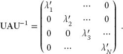
The diagonal values of UAU⁻¹ are the eigenvalues with eigenvectors

(6.28)

that is, the eigenvectors are the columns of the matrix U⁻¹. A number of routines of this type are found in subroutine libraries.

6.3.1 Practical Matrix Computing

Many scientific programming bugs arise from the improper use of arrays.³⁾ This may be as a result of the extensive use of matrices in scientific computing or to the complexity of keeping track of indices and dimensions. In any case, here are some rules of thumb to observe.

Computers are finite Unless you are careful, your matrices may so much memory that your computation will slow down significantly, especially if it starts to use virtual memory. As a case in point, let us say that you store data in a 4D array with each index having a physical dimension of 100: A[100] [100] [100] [100]. This array of (100)⁴ 64-byte words occupies :1 GB of memory.

Processing time Matrix operations such as inversion require on the order of N³ steps for a square matrix of dimension N. Therefore, doubling the dimensions of a 2D square matrix (as happens when the number of integration steps is doubled) leads to an eightfold increase in the processing time.

Paging Many operating systems have virtual memory in which disk space is used when a program runs out of RAM (see Chapter 10) for a discussion of how computers arrange memory). This is a slow process that requires writing a full page of words to the disk. If your program is near the memory limit at which paging occurs, even a slight increase in a matrix’s dimension may lead to an order of magnitude increase in the execution time.

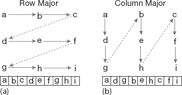
Figure 6.3 (a) Row-major order used for matrix storage in Python, C and Java. (b) Column-major order used for matrix storage in Fortran. The table at the bottom shows how successive matrix elements are actually stored in a linear fashion in memory.

Matrix storage While we think of matrices as multidimensional blocks of stored numbers, the computer stores them as linear strings. For instance, a matrix a[3,3] in Python, is stored in row-major order (Figure 6.3a):

(6.29)

while in Fortran, starting subscripts at 0, it is stored in column-major order (Figure 6.3b):

(6.30)

It is important to keep this linear storage scheme in mind in order to write proper code and to permit the mixing of Python and Fortran programs.

When dealing with matrices, you have to balance the clarity of the operations being performed against the efficiency with which the computer performs them. For example, having one matrix with many indices such as V[L,Nre,Nspin,k,kp,Z,A] may be neat packaging, but it may require the computer to jump through large blocks of memory to get to the particular values needed (large strides) as you vary k, kp, and Nre. The solution would be to have several matrices such as V1[Nre,Nspin,k,kp,Z,A], V2[Nre,Nspin,k,kp,Z,A], and V3[Nre,Nspin,k,kp,Z,A].

Subscript 0 It is standard in Python, C, and Java to have array indices begin with the value 0. While this is now permitted in Fortran, the standard in Fortran and in most mathematical equations has been to start indices at 1. On that account, in addition to the different locations in memory as a result of row-major and column-major ordering, the same matrix element may be referenced differently in the different languages:

Location	Python/C element	Fortran element
Lowest	a [0,0]	a (1,1)
	a [0,1]	a (2,1)
	a [1,0]	a (3,1)
	a [1,1]	a (1,2)
	a [2,0]	a (2,2)
Highest	a [2,1]	a (3,2)

Tests Always test a library routine on a small problem whose answer you know (such as the exercises in Section 6.6). Then you will know if you are supplying it with the right arguments and if you have all the links working.

6.4 Python Lists as Arrays

A list is Python’s built-in sequence of numbers or objects. Although called a “list” it is similar to what other computer languages call an “array.” It may be easier for you to think of a Python list as a container that holds a bunch of items in a definite order. (Soon we will describe the higher level array data types available with the NumPy package.) In this section we review some of Python’s native list features. Python interprets a sequence of ordered items, L = l₀, l₁, … , l_N−1, as a list and represents it with a single symbol L:

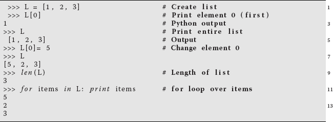
We observe that square brackets with comma separators [1, 2, 3] are used for lists, and that a square bracket is also used to indicate the index for a list item, as in line 2 (L[0]). Lists contain sequences of arbitrary objects that are mutable or changeable. As we see in line 7 in the L command, an entire list can be referenced as a single object, in this case to obtain its printout.

Python also has a built-in type of list known as a tuple whose elements are not mutable. Tuples are indicated by round parenthesis (.., .., .), with individual elements still referenced by square brackets:

Note that the error message arises when we try to change an element of a tuple.

Most languages require you to specify the size of an array before you can start storing objects in it. In contrast, Python lists are dynamic, which means that their sizes adjust as needed. In addition, while a list is essentially one dimensional because it is a sequence, a compound list can be created in Python by having the individual elements themselves as lists:

Python can perform a large number of operations on lists, for example,

Operation	Effect	Operation	Effect
L = [1, 2, 3, 4]	Form list	L1 + L2	Concatenate lists
L[i]	ith element	len(L)	Length of list L
i in L	True if i in L	L[i:j]	Slice from i to j
for i in L	Iteration index	L.append(x)	Append x to end of L
L.count(x)	Number of x’s in L	L.index(x)	Location of 1st x in L
L.remove(x)	Remove 1st x in L	L.reverse()	Reverse elements in L
L.sort()	Order elements in L

6.5 Numerical Python (NumPy) Arrays

Although basic Python does have an array data type, it is rather limited and we suggest using NumPy arrays, which will convert Python lists into arrays. Because we often useNumPy’s array command to form computer representations of vectors and matrices, you will have to import NumPy in your programs (or Visual, which includes NumPy) to use those examples. For instance, here we show the results of running our program Matrix.py from a shell:

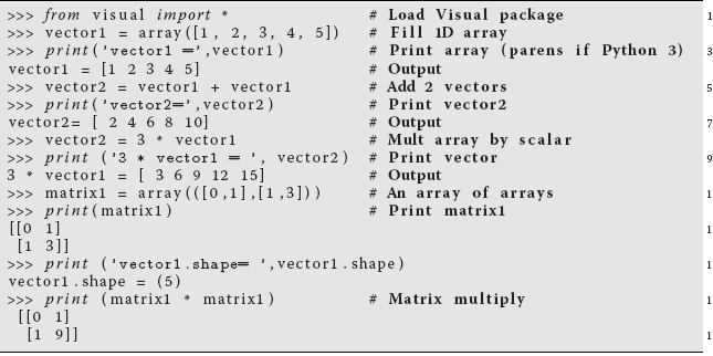
We see here that we have initialized an array object, added two 1D array objects together, and printed out the result. Likewise we see that multiplying an array by a constant does in fact multiply each element by that constant (line 8). We then construct a “matrix” as a 1D array of two 1D arrays, and when we print it out, we note that it does indeed look like a matrix. However, when we multiply this matrix by itself, the result is not that one normally expects from matrix multiplication. So if you need actual mathematical matrices, then you need to use NumPy!

Now we give some examples of the use of NumPy, but do refer the reader to the NumPy Tutorial (NumPyTut, 2012) and to the articles in Computing in Science and Engineering (Perez et al., 2010) for more information. To start, we note that a NumPy array can hold up to 32 dimensions (32 indices), but each element must be of the same type (a uniform array). The elements are not restricted to just floatingpoint numbers or integers, but can be any object, as long as all elements are of this same type. (Compound objects may be useful, for example, for storing parts of data sets.) There are various ways to create arrays, with square brackets […] used for indexing in all cases. First we start with a Python list (tuples work as well) and create an array from it:

Notice that it is essential to have the square brackets within the round brackets because the square brackets produce the list object while the round brackets indicate a function argument. Note also that because the data in our original list were all integers, the created array is a 32-bit integer data types, which we can check by affixing the dtype method:

If we had started with floating-point numbers, or a mix of floats and ints, we would have ended up with floating-point arrays:

When describing NumPy arrays, the number of “dimensions,” ndim, means the number of indices, which, as we said, can be as high as 32. What might be called the “size” or “dimensions” of a matrix in mathematics is called the shape of a NumPy array. Furthermore, NumPy does have a size method that returns the total number of elements. Because Python’s lists and tuples are all one dimensional, if we want an array of a particular shape, we can attain that by affixing the reshape method when we create the array. Where Python has a range function to generate a sequence of numbers, NumPy has an arange function that creates an array, rather than a list. Here we use it and then reshape the 1D array into a 3 × 4 array:

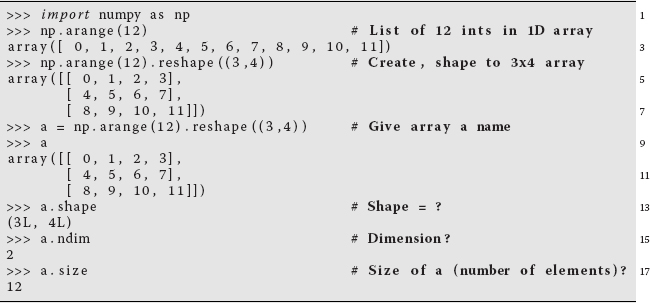
Note that here we imported NumPy as the object np, and then affixed the arange and reshape methods to this object. We then checked the shape of a, and found it to have three rows and four columns of long integers (Python 3 may just say ints). Note too, as we see on line 9, NumPy uses parentheses () to indicate the shape of an array, and so (3L,4L) indicates an array with three rows and four columns of long ints.

Now that we have shapes in our minds, we should note that NumPy offers a number of ways to change shapes. For example, we can transpose an array with the .T method, or reshape into a vector:

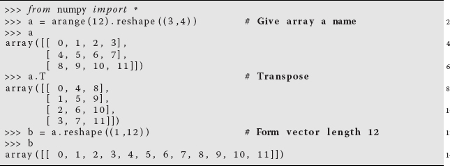
And again, (1,12) indicates an array with 1 row and 12 columns. Yet another handy way to take a matrix and extract just what you want from it is to use Python’s slice operator start:stop:step: to take a slice out of an array:

We note here that Python indices start counting from 0, and so 1:3 means indices 0, 1, 2 (without 3). As we discuss in Chapter 11, slicing can be very useful in speeding up programs by picking out and placing in memory just the specific data elements from a large data set that need to be processed. This avoids the time-consuming jumping through large segments of memory as well as excessive reading from disk.

Finally, we remind you that while all elements in a NumPy array must be of the same data type, that data type can be compound, for example, an array of arrays:

Furthermore, an array can be composed of complex numbers by specifying the complex data type as an option on the array command. NumPy then uses the j symbol for the imaginary number i:

In the next section, we discuss using true mathematical matrices with NumPy, which is one use of an array object. Here we note that if you wanted the familiar matrix product from two arrays, you would use the dot function, whereas * is used for an element-by-element product:

NumPy is actually optimized to work well with arrays, and in part this is because arrays are handled and processed much as if they were simple, scalar variables.⁴⁾ For example, here is another example of slicing, a technique that is also used in ordinary Python with lists and tuples, in which two indices separated by a colon indicate a range:

Here we start by creating the NumPy array stuff of floats, all of whose 10 elements are initialized to zero. Then we create the array t containing the four elements [0, 1, 2, 3] by assigning four variables uniformly in the range 0–4 (the “a” in arange creates floating-point variables, range creates integers). Next we use a slice to assign [sqrt(0+1), sqrt(1+1), sqrt(2+1), sqrt(3+1)] = [1, 1.414, 1.732, 2] to the middle elements of the stuff array. Note that the NumPy version of the sqrt function, one of many universal functions (ufunctions) supported by NumPy⁵⁾, has the amazing property of automatically outputting an array whose length is that of its argument, in this case, the array t. In general, major power in NumPy comes from its broadcasting operation, an operation in which values are assigned to multiple elements via a single assignment statement. Broadcasting permits Python to vectorize array operations, which means that the same operation can be performed on different array elements in parallel (or nearly so). Broadcasting also speeds up processing because array operations occur in C instead of Python, and with a minimum of array copies being made. Here is a simple sample of broadcasting:

The first line creates the NumPy array w, and the second line “broadcasts” the value 23.7 to all elements in the array. There are many possible array operations in NumPy and various rules pertaining to them; we recommend that the serious user explore the extensive NumPy documentation for additional information.

6.5.1 NumPy’s linalg Package

The array objects of NumPy and Visual are not the same as mathematical matrices, although an array can be used to represent a matrix. Fortunately, there is the LinearAlgebra package that treats 2D arrays (a 1D array of 1D arrays) as mathematical matrices, and also provides a simple interface to the powerful LAPACK linear algebra library (Anderson et al., 2013). As we keep saying, there is much to be gained in speed and reliability from using these libraries rather than writing your own matrix routines.

Our first example from linear algebra is the standard matrix equation

(6.31)

where we have used an uppercase bold character to represent a matrix and a lowercase bold italic character to represent a 1D matrix (a vector). Equation 6.31 describes a set of linear equations with x an unknown vector and A a known matrix. Now we take y yA to be 3 × 3, b to be 3 × 1, and let the program figure out that x must be a 3 × 1 vector.⁶⁾ We start by importing all the packages, by inputting a matrix and a vector, and then by printing out A and x:

Because we have the matrices A and b, we can go ahead and solve Ax = b using NumPy’s solve command, and then test how close Ax − b is to a zero vector:

This is really quite impressive. We have solved the entire set of linear equations (by elimination) with just the single command solve, performed a matrix multiplication with the single command dot, did a matrix subtraction with the usual operator, and are left with a residual essentially equal to machine precision.

Although there are more efficient numerical approaches, a direct way to solve

(6.32)

is to calculate the inverse A⁻¹, and then multiply both sides of the equation by the inverse, yielding

(6.33)

Here we first tested that inv(A) is in fact the inverse of A by seeing if A times inv(A) equals the identity matrix. Then we used the inverse to solve the matrix equation directly, and got the same answer as before (some error at the level of machine precision is just fine).

Our second example occurs in the solution for the principal-axes system of a cube, and requires us to find a coordinate system in which the inertia tensor is diagonal. This entails solving the eigenvalue problem

(6.34)

where I is the inertia matrix (tensor), ω is an unknown eigenvector, and λ is an unknown eigenvalue. The program Eigen.py solves for the eigenvalues and vectors, and shows how easy it is to deal with matrices. Here it is in an abbreviated interpretive mode:

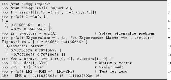
Table 6.1 The operators of NumPy and their effects.

Operator	Effect	Operator	Effect
dot(a, b[,out])	Dot product arrays	vdot(a, b)	Dot product
inner(a, b)	Inner product arrays	outer(a, b)	Outer product
tensordot(a, b)	Tensor dot product	einsum()	Einstein sum
linalg.matrix_power(M, n)	Matrix to power n	kron(a, b)	Kronecker product
linalg.cholesky(a)	Cholesky decomp	linalg.qr(a)	QR factorization
linalg.svd(a)	Singular val decomp	linalg.eig(a)	Eigenproblem
linalg.eigh(a)	Hermitian eigen	linalg.eigvals(a)	General eigen
linalg.eigvalsh(a)	Hermitian eigenvals	linalg.norm(x)	Matrix norm
linalg.cond(x)	Condition number	linalg.det(a)	Determinant
linalg.slogdet(a)	Sign and log(det)	trace(a)	Diagnol sum
linalg.solve(a, b)	Solve equation	linalg.tensorsolve(a, b)	Solve ax = b
linalg.lstsq(a, b)	Least-squares solve	linalg.inv(a)	Inverse
linalg.pinv(a)	Penrose inverse	linalg.tensorinv(a)	Inverse N–D array

We see here how, after we set up the array I on line 3, we then solve for its eigenvalues and eigenvectors with the single statement Es, evectors = eig(I) on line 8. We then extract the first eigenvector on line 14 and use it, along with the first eigenvalue, to check that (6.34) is in fact satisfied to machine precision.

Well, we think by now you have some idea of the use of NumPy. In Table 6.1 we indicate some more of what is available.

6.6 Exercise: Testing Matrix Programs

Before you direct the computer to go off crunching numbers on a million elements of some matrix, it is a good idea to try out your procedures on a small matrix, especially one for which you know the right answer. In this way, it will take you only a short time to realize how hard it is to get the calling procedure perfect. Here are some exercises.

1. Find the numerical inverse of .
   1. a) As a general check, applicable even if you do not know the analytic answer, check your inverse in both directions; that is, check that AA⁻¹ = A⁻¹A = I, and note the number of decimal places to which this is true. This also gives you some idea of the precision of your calculation.
   2. b) Determine the number of decimal places of agreement there is between your numerical inverse and the analytic result:
      Is this similar to the error in AA⁻¹?
2. Consider the same matrix A as before, here being used to describe three simultaneous linear equations, Ax = b, or explicitly,
   
   (6.35)
   
   Now the vector b on the RHS is assumed known, and the problem is to solve for the vector x. Use an appropriate subroutine to solve these equations for the three different x vectors appropriate to these three different b values on the RHS:
   

   

   
   The solutions should be
   
   (6.36)
3. Consider the matrix , where you are free to use any values you want for α and β. Use a numerical eigenproblem solver to show that the eigenvalues and eigenvectors are the complex conjugates:
   (6.37)
4. Use your eigenproblem solver to find the eigenvalues of the matrix
   (6.38)
   1. a) Verify that you obtain the eigenvalues λ₁ = 5, λ₂ = λ₃ = −3. Notice that double roots can cause problems. In particular, there is a uniqueness issue with their eigenvectors because any combination of these eigenvectors is also an eigenvector.
   2. b) Verify that the eigenvector for λ₁ = 5 is proportional to
      (6.39)
   3. c) The eigenvalue −3 corresponds to a double root. This means that the corresponding eigenvectors are degenerate, which in turn means that they are not unique. Two linearly independent ones are
      (6.40)
      
      In this case, it is not clear what your eigenproblem solver will give for the eigenvectors. Try to find a relationship between your computed eigenvectors with the eigenvalue −3 and these two linearly independent ones.
5. Imagine that your model of some physical system results in N = 100 coupled linear equations in N unknowns:
   
   
   
   In many cases, the a and b values are known, so your exercise is to solve for all the x values, taking a as the Hilbert matrix and b as its first column:
   
   
   
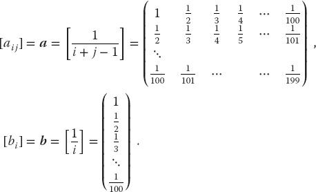
   Compare to the analytic solution
   (6.41)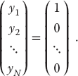
6. Dirac Gamma Matrices: The Dirac equation extends quantum mechanics to include relativity and spin 1/2. The extension of the Hamiltonian operator for an electron requires it to contain matrices, and those matrices are expressed in terms of 4 × 4 γ matrices that can be represented in terms of the familiar 2 × 2 Pauli matrices σ_i:
   (6.42)
   (6.43)
   
   Confirm the following properties of the γ matrices:
   
   (6.44)
   (6.45)

6.6.1 Matrix Solution of the String Problem

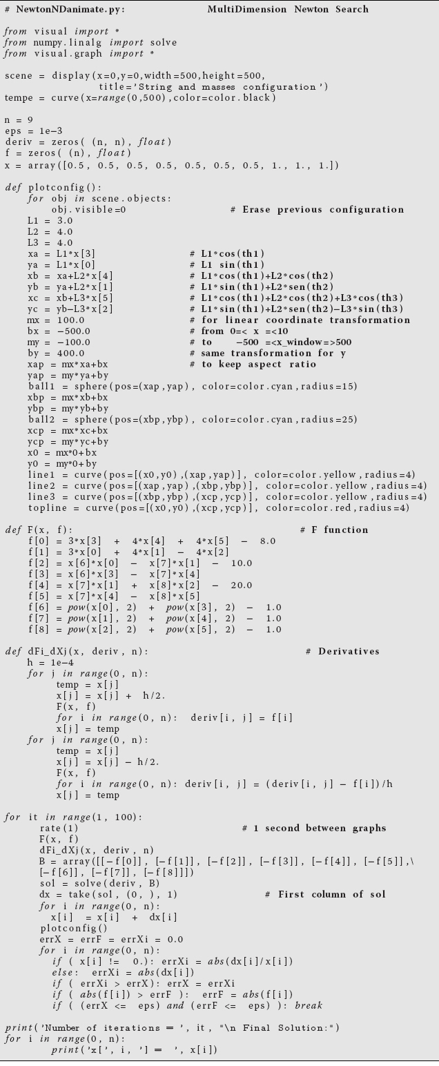
In Section 6.1, we set up the solution to our problem of two masses on a string. Now we have the matrix tools needed to solve it. Your problem is to check out the physical reasonableness of the solution for a variety of weights and lengths. You should check that the deduced tensions are positive and the deduced angles correspond to a physical geometry (e.g., with a sketch). Because this is a physics-based problem, we know the sine and cosine functions must be less than 1 in magnitude and that the tensions should be similar in magnitude to the weights of the spheres. Our solution is given in NewtonNDanimate.py (Listing 6.1), which shows graphically the step-by-step search for a solution.

Listing 6.1 The code NewtonNDanimate.py that shows the step-by-step search for solution of the two-mass-on-a-string problem via a Newton–Raphson search.

6.6.2 Explorations

1. See at what point your initial guess for the angles of the strings gets so bad that the computer is unable to find a physical solution.
2. A possible problem with the formalism we have just laid out is that by incorporating the identity sin² θ_i + cos² θ_i = 1 into the equations, we may be discarding some information about the sign of sin θ or cos θ. If you look at Figure 6.1, you can observe that for some values of the weights and lengths, θ₂ may turn out to be negative, yet cos θ should remain positive. We can build this condition into our equations by replacing f₇−f₉ with f’s based on the form
   (6.46)
   
   See if this makes any difference in the solutions obtained.
3. Solve the similar three-mass problem. The approach is the same, but the number of equations is larger.

1) Almost impossible anyway, as L. Molnar has supplied me with an analytic solution.

2) Although we prize the book, Numerical Recipes by Press et al. (1994), and what it has accomplished, we cannot recommend taking subroutines from it. They are neither optimized nor documented for easy, stand-alone use, whereas the subroutine libraries recommended in this chapter are.

3) Even a vector V(N) is called an array, albeit a 1D one.

4) We thank Bruce Sherwood for helpful comments on these points.

5) A ufunction is a function that operates on N–D arrays in an element-by-element fashion, supporting array broadcasting, type casting, and several other standard features. In other words, a ufunc is a vectorized wrapper for a function that takes a fixed number of scalar inputs and produces a fixed number of scalar outputs.

6) Do not be bothered by the fact that although we think these vectors as 3 × 1, they sometimes get printed out as 1 × 3; think of all the trees that get saved!