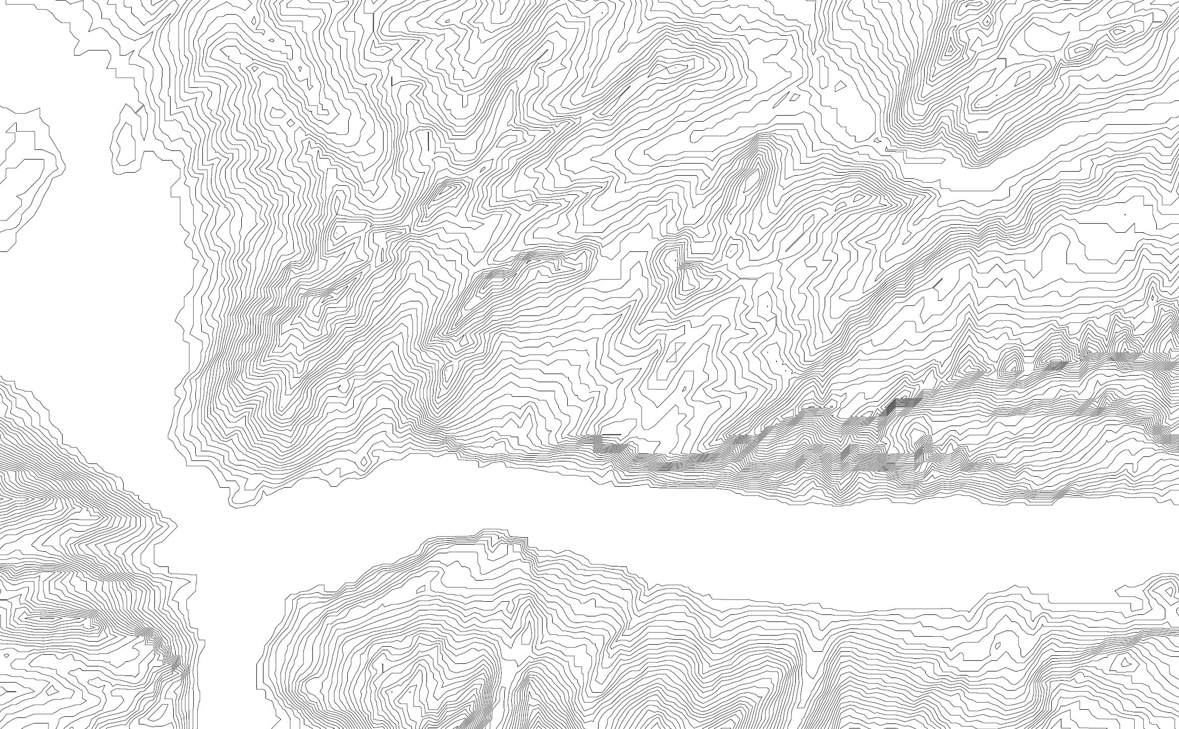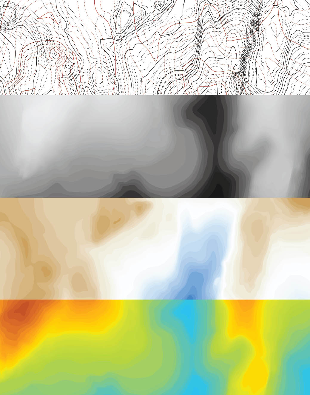
2.1
40.7823° N, 73.9658° W, Jill Desimini, Contour Techniques: Central Park Lake, 2014. After Jean-Charles Adolphe Alphand [FIG. 2.12], OLM et al. [FIG. 2.14], International Hydrographic Organization [FIG. 2.7], and NOAA [FIG. 2.9].
Lines joining points of equal vertical distance above or below a datum.
The contour line, a member of the isoline family, is the representational staple of topographical description and projection. The line is an abstraction of altitude, connecting points of equal elevation. Nonexistent in the landscape, the contour traces a horizontal slice through topography. In a drawing of terrain—be it a topographic map or a grading plan—contours are spaced at a given vertical interval determined by the scale of the drawing and the intricacies of the depicted landscape. The result is a series of lines, a single-weave fabric depicting the morphological characteristics of the ground. Tight offsets and densely packed lines describe steep slopes, while wide gaps between lines indicate flatness.
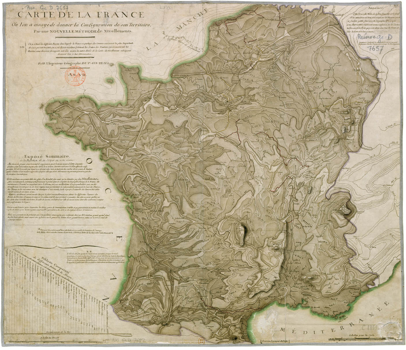
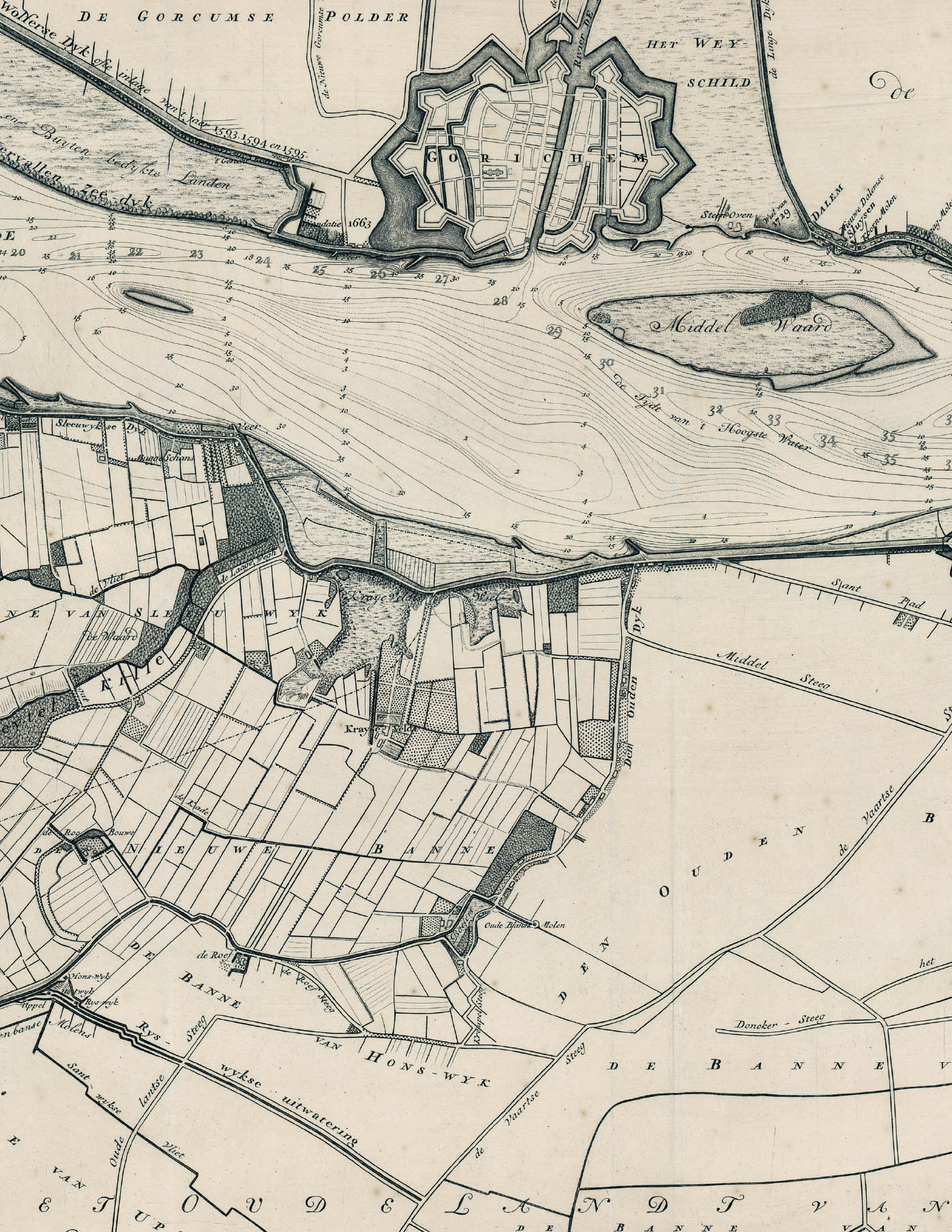
Commonly thought of as a terrestrial convention, the contour evolved from its aqueous father, the isobath. The first isolines were used in bathymetrical charts to describe the depths of river mouths, inlets, and bays, unseen ground whose whereabouts are crucial for navigational success. Emerging from Dutch and French traditions, these early contours were smoothly abstracted from soundings (SEE CHAPTER 01), creating the impression of a soft, water floor, lightly articulated against the hard edges of the adjacent built environment. The early contour maps of landmasses translated this innovative approach to describing fluvial geomorphology to terrestrial landform. The French were again innovators, producing what is recognized as the earliest contour mapping. While looping, scalloped, and at wide interval, Jean-Louis Dupain-Triel’s 1798–99 Carte de la France depicts a surface with lines circumscribing landmass, drawing form out of fields of spot elevations in a manner devoid of some of the subjectivity of intuitive shading and pictograms. The layers read strongly, as extruded levels, with the distinct shapes of the contours emphasized rather than the mountainous masses they represent. In French, a contour map is a carte en courbes de niveau, or a “map of curves at a given level.”
Early contours were highly generalized, but the efficacy and potential of the system was quickly understood. As Swiss cartographer Eduard Imhof noted, “The contour is the most important element in cartographic representation of the terrain and the only one that determines relief forms geometrically.”1 It forms the basis for other modes of representation, including hachures (SEE CHAPTER 03) and shaded relief (SEE CHAPTER 04), as well as the foundation for grading and landform design. Landscape architects manipulate contours on paper and screen to envision, describe, and dictate the moving of earth and material in the field.
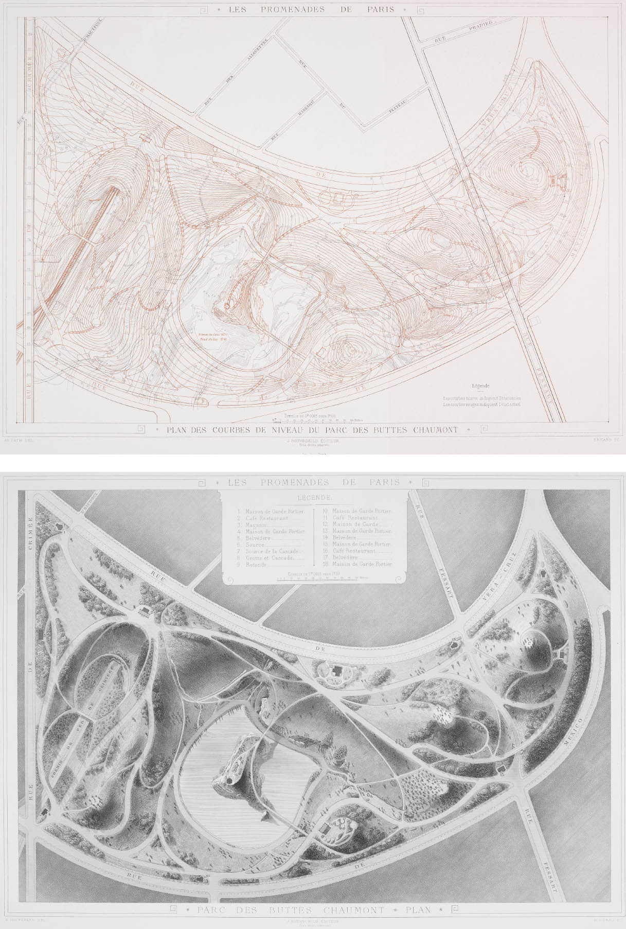
The emphasis on the contour plan as a technical tool to describe and manipulate the surface of the earth remained central in French design culture and technical education. At the École des Ponts et Chaussées, the early pedagogy centered on the drawing of maps, emphasizing that the reading and drawing of the countryside was essential to the engineering profession and that the plan was the basis of all projects.2 Jean-Charles Adolphe Alphand, chief engineer of parks under Georges Eugène Haussmann and Napoléon III, was trained in this tradition. His work at the Parc des Buttes Chaumont (1867) represented the use of the map, and more specifically the contour plan, as a means to conquer and transform space. Here, the contour becomes a tool to exploit technical mastery, re-envision urban fabric, and mobilize quick construction. By including a contour plan of the park in the publicly distributed series of promotional illustrations, Promenades de Paris, Alphand demonstrated the skill and precision underlying the ambitious Parc des Buttes Chaumont project. [FIG. 2.12] Paired with a rich and dramatic engraving of the park, the contour plan showed the before and after contours, mathematically indicating the cut and fill required for construction. The abstract language of contours may not have been legible to the general consumer, but the impressive drawing bred faith in the technical abilities of the government efforts. Further, Alphand could use the contour calculations to estimate and order materials, facilitating the construction process.3 Grading plans indicating the displacement between existing and proposed contours continue to be used to design and build landforms, with greater precision and automation providing transfer from design vision to constructed landscape.
In cartography, the contour has evolved from a highly generalized and expressive line, drawn by connecting a few points of known elevation to a carefully calibrated mathematical articulation of form derived from detailed and accurate surveys. The tools of surveying and representation have allowed for greater precision, challenging cartographers to advance scientific knowledge without alienating themselves from an intimate understanding of the feel, material, and texture of the ground. Increased accuracy of data makes possible further freedom of expression.
Similarly, in design practice, the contour has been liberated from its technical chains. After a long period of service, for which the contour was used primarily as a construction tool to execute a design conceived through other means of articulating topography (e.g., spot elevations, shading, sections, perspectives, models), the contour line has recently reemerged as a projective element in the creative process. It has become a way of organizing space, of articulating topography as the main driver of a project, and of expressing the integration of site and building. It evokes the qualitative characteristics of the landform it describes through color, form, and gestural means.
The representation of the contour began as a thin black line but has embraced a number of techniques throughout history. Like other forms of cartographic conventions, no singular representational system has emerged. Distinctions are often made between existing and proposed contours—dashed and solid, light and dark, noncolored and colored. Index contours, usually assigned to every fifth contour to facilitate legibility, can be darker than intermediate contours. Gradients can be introduced to go from low to high or high to low. Line color can also be used to distinguish material quality—black for rocks, blue for water or glaciers, brown for earthen and vegetated areas. Numbering can appear within the line or between two lines; the number in this case represents the lower elevation value.
Hypsometric tints—or color ramps—can fill the contours to further emphasize the topographic progression. In bathymetric conventions, the fill dominates. Older maps espoused a ramp of blues to simulate depth, whereas newer conventions have at times strayed from material verisimilitude to independent schemes—a ROYGBIV rainbow reading from low to high—joining a robust set of thematic heat maps that use the ROYGBIV spectrum to indicate data variations.
Each technique achieves different affects [FIG. 2.1]. The overlays of existing and proposed contours allow for the reading of the design transformation, integrating time into the drawing. A blue and tan ramp creates a clear distinction between topographic and bathymetric elevations in a subtle color scheme. The grayscale and ROYGBIV versions do not distinguish between land and water, presenting a continuous surface in tonal and color schemes that lack mimicry and highlight the contoured levels. Despite all the difference and variation, topographic maps across countries often land on dark or reddish brown as the choice color for contours. United States Geological Survey contours are brown; Swiss contours are reddish brown, as are Japanese, Indonesian, Nepalese, Bahraini, Korean, and French, to name a few others (SEE NOTES ON SCALE). Black is the most readily available printing color, but the effect can be harsh. Dark or reddish brown contrasts nicely with black, blue, green, and white, the other dominant colors of topographic description, without overpowering the representation. In design drawings, brown contours are rare, black and gray are most prevalent, white appears on dark backgrounds, and warm red or orange makes appearances. Design, as compared to cartography, permits greater representational freedom and with it the opportunity for a range of interpretation in the use, identity, and formation of the contour line. The following examples trace the representational trends and variations across time, media, and subject.
1Eduard Imhof, Cartographic Relief Presentation (Redlands, CA: Esri, 2007), 111.
2Antoine Picon, French Architects and Engineers in the Age of Enlightenment (Cambridge, UK: Cambridge University Press, 2010).
3Ann E. Komara, “Measure and Map: Alphand’s Contours of Construction at the Parc des Buttes Chaumont, Paris 1867,” Landscape Journal 28, no. 1 (2009): 22–39.
2.1
40.7823° N, 73.9658° W, Jill Desimini, Contour Techniques: Central Park Lake, 2014. After Jean-Charles Adolphe Alphand [FIG. 2.12], OLM et al. [FIG. 2.14], International Hydrographic Organization [FIG. 2.7], and NOAA [FIG. 2.9].
2.3
46.0000° N, 2.0000° E, Jean-Louis Dupain-Triel Jr. and J. B. Dien, Carte de la France, 1798–99.
Jean-Louis Dupain-Triel Jr. produced the first contour map of France in 1791, one of the earliest examples of terrestrial contours. The map was republished in 1799 (pictured) and included stylized, scalloped contours at ten-meter intervals. With the distribution of this map, Dupain-Triel successfully lobbied for the contour as a standard of topographic representation.
2.4
18.4517° N, 66.0689° W, James Corner Field Operations, University of Puerto Rico Botanical Gardens, 2003–6. Scale: 1:2,500 (shown at half size).
The plan of the University of Puerto Rico Botanical Gardens comprises flat swaths of color that imply topography as an underlying condition of the design work. The design itself is organized into three layers: surface fields, or mats; circulation loops; and forest plantings. The articulation of these layers reveals the topographic particularities of the site: larger swaths in the flood-prone flat land of the north; a more intricate, at times concentric language responding to the varied slopes in the south; and a set of offset ribbons along the central riverine corridor describing the subtle slopes of the spreading banks.
2.5
51.8167° N, 4.6667° E, Nicolaas Cruquius, De Rivier de Merwede, ca. 1730. Scale: approx. 1:10,000 (shown at half size).
As waterborne transport increased, systematic advances in measuring navigable channels began to proliferate. With much of its land below sea level, the Netherlands was understandably at the forefront of fluvial surveying. Dutch surveyor Nicolaas Cruquius was a pioneer in the field, and his yearlong mapping of the mouth of the Meuse River demonstrates his innovative use of contour lines to depict the shape of the river bottom. The drawing is remarkable both for its technical prowess and for the way the thin bathymetric lines evoke the ephemeral qualities of the water, especially when juxtaposed with the heavy line weights of the fortified bank.
2.6
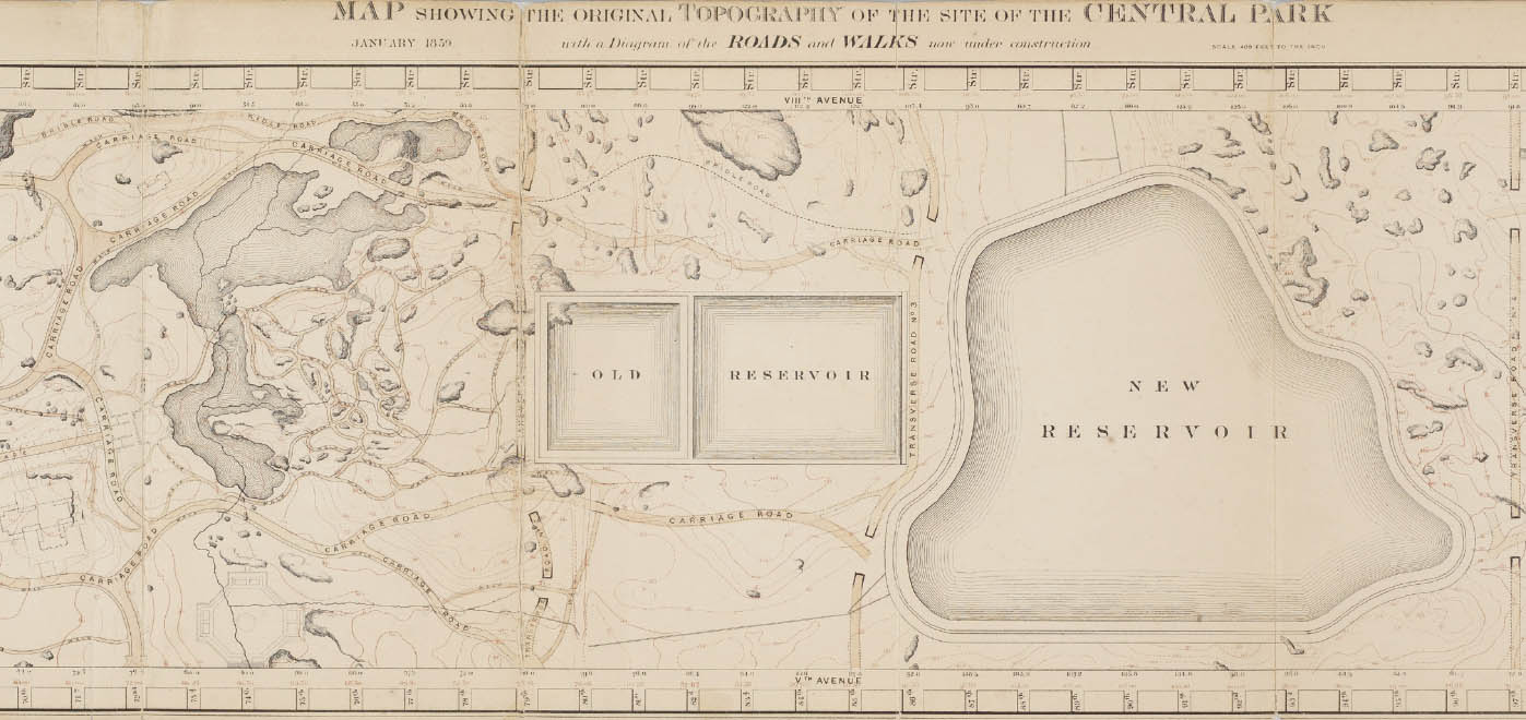
40.7823° N, 73.9658° W, Frederick Law Olmsted and Calvert Vaux, Map Showing the Original Topography of the Site of the Central Park, 1859.
In contrast to the presentation drawing of the competition-winning Greensward Plan of 1858 by Frederick Law Olmsted and Calvert Vaux, a deceivingly flat representation, the original topography plan shown here clearly demonstrates the extensive earthwork required to construct the park, to make it suitable for public recreation. Olmsted’s park presentation drawings, like the Greensward Plan, did not include contour lines. Contour lines were reserved for the technical drawings used to dictate construction rather than the imaginative ones used to envision design. This map of the original topography was included in the Second Annual Report of the Board of Commissioners of the Central Park.
2.7
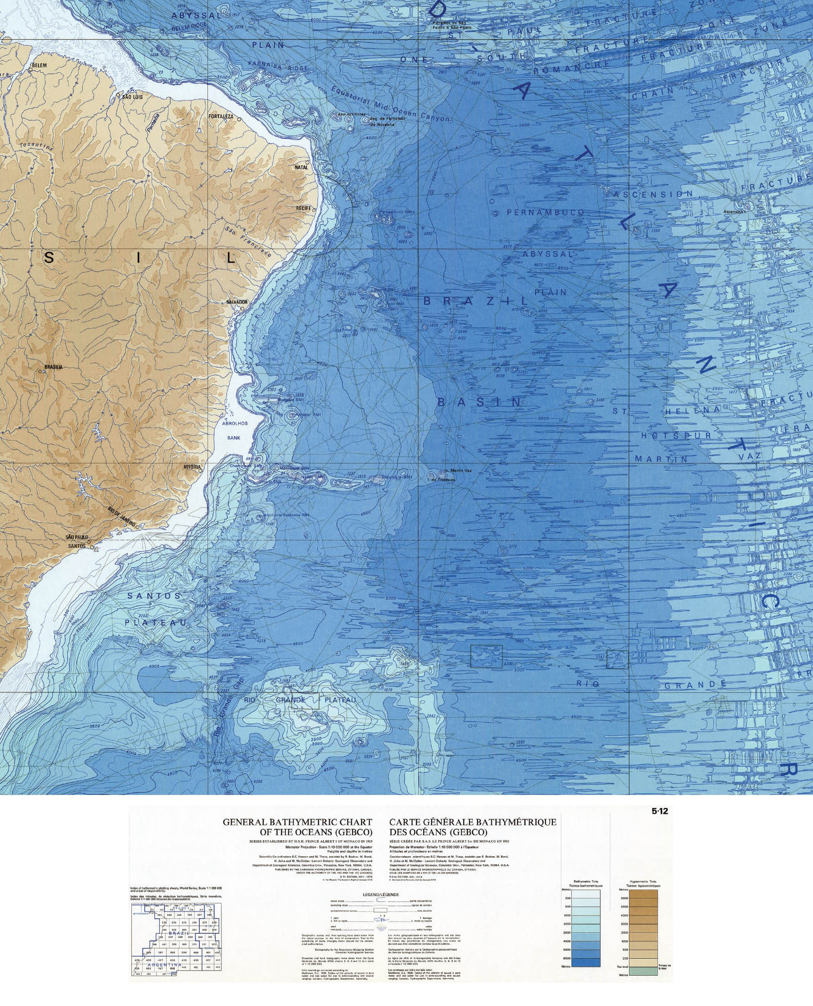
38.4667° N, 28.4000° W, International Hydrographic Organization, General Bathymetric Chart of the Oceans 5.12, 1978. Scale: 1:10,000,000 (shown at half size).
The hypsometric color ramp of the General Bathymetric Chart of the Oceans draws inspiration from the soft hues—blues, yellows, and grays—of the clouds and the sky. As the graphically astute Edward Tufte describes, the chart “records ocean depth (bathymetric tints) and land height (hypsometric tints) in twenty-one steps—with ‘the deeper or higher, the darker’ serving as the visual metaphor for coloring. . . . Every color mark on this map signals four variables: latitude, longitude, sea or land, and depth or altitude measured in meters.” The result is strikingly clear and resoundingly beautiful.
2.8
43.6725° N, 1.3472° W, Agence Patrick Arotcharen and Estudi Martí Franch, Les Echasses Golf and Surf Nature Resort, 2013.
The plan of Les Echasses resort by Estudi Martí Franch, a Barcelona-based landscape architecture firm, draws clear inspiration from cartographic techniques. The project is driven by topographic manipulation, and the representation supports this emphasis on landform. Beginning with a flat cornfield site, the designers created an intricate lake and dunescape to maximize water access. The combination of hypsometric and bathymetric tints with hatches expands and blurs the line between land and water.
2.9
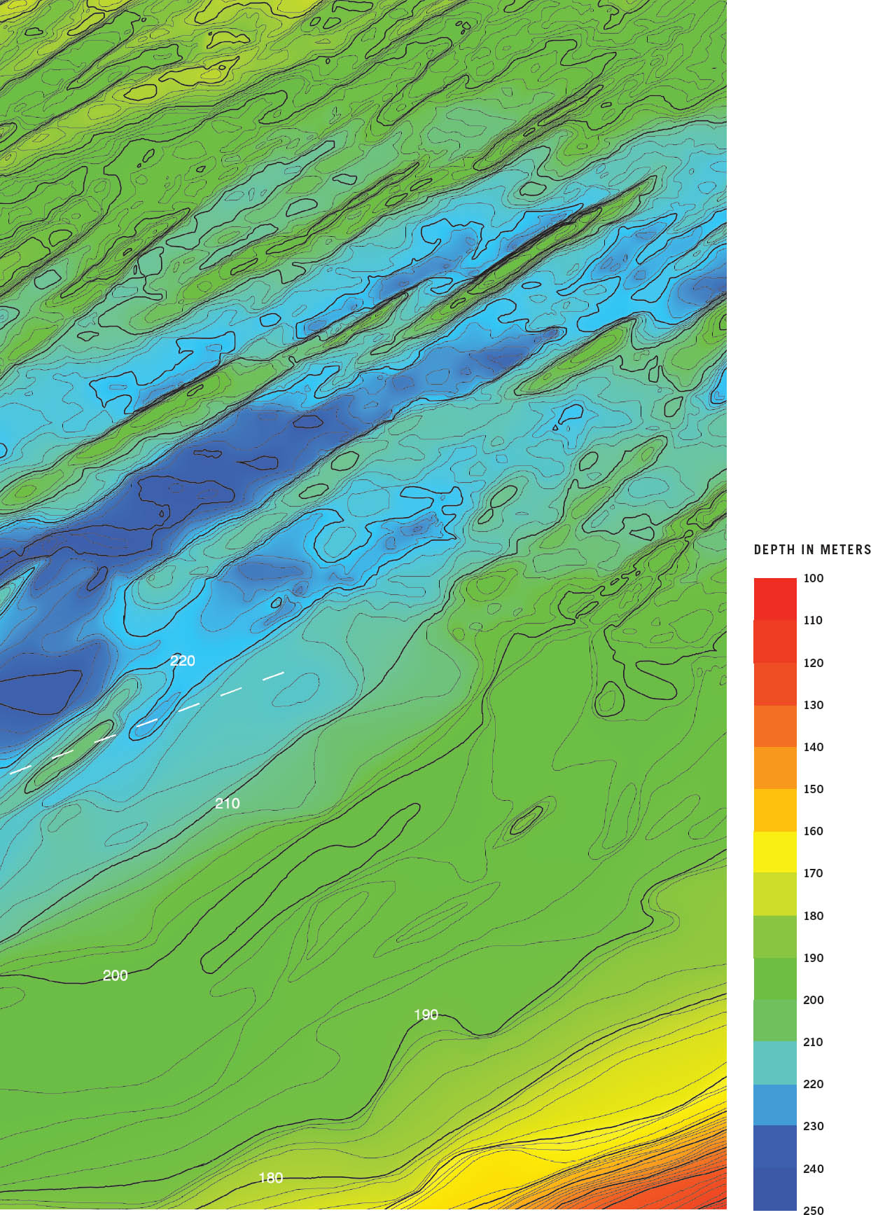
43.7000° N, 77.9000° W, National Oceanic and Atmospheric Administration (NOAA), Great Lakes Data Rescue Project-Lake Ontario Bathymetry: Rochester Basin, 2000. Scale: 1:50,000 (shown at half size).
A heat map is a graphical representation of data whereby different values are assigned different colors. The ROYGBIV color scheme is common though not prescribed. Ubiquitous in thematic mapping, the heat-map visualization can be applied to contour mapping through the tradition of hypsometric tints. In data visualization, the heat map can be interpolated from discontinuous data to create a surface, whereas in contour mapping, the ramp gradient reflects the continuity of the terrain.
2.10
40.6905° N, 74.0165° W, West 8 Urban Design and Landscape Architecture, Governors Island Park and Public Space Master Plan, 2007–13.
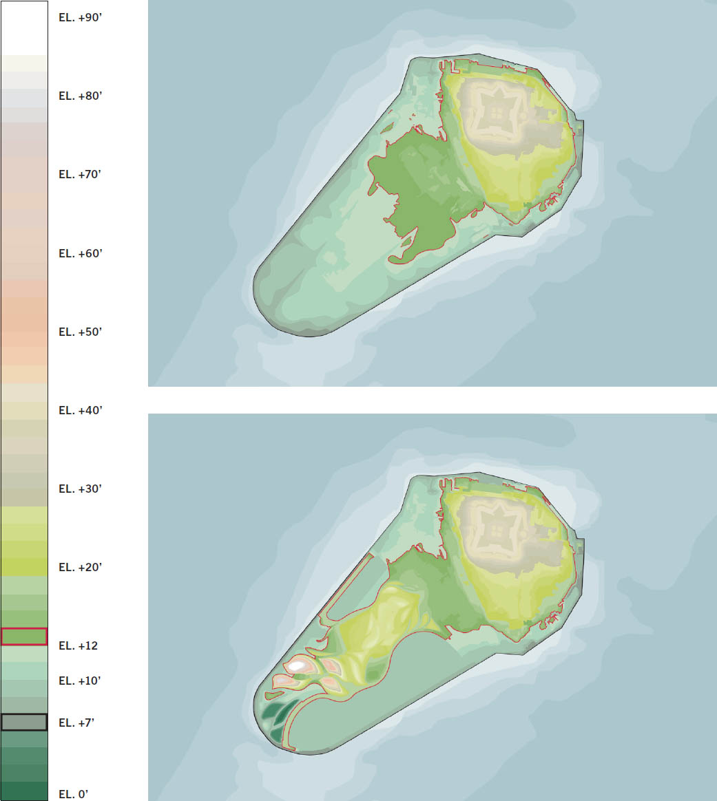
The West 8 hypsometric ramp presents elevation levels with different hues, rather than tonal variations of a single hue. Blues and greens are low elevations, yellows are mid elevations, and grays are higher elevations. This color scheme emphasizes the topographic changes from existing to proposed, highlighting the new raised landforms in the southern portion of the island.
2.11
24.1470° N, 120.6744° E, Stoss Landscape Urbanism, Taichung Gateway Park, 2012.
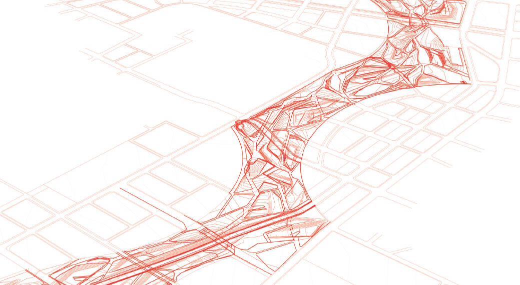
Extracted from a three-dimensional model, the proposed contours of Stoss’s Taichung Gateway Park describe a syncopated, water-driven landscape. The cuts create basins to capture, clean, and ultimately program Taiwan’s voluminous rainfall. The perspectival view of the contours animates the shifts in topography across the linear park, allowing the eye to wander, to imagine the movement of rain and park visitors alike.
2.12
48.8742° N, 2.3470° E, Jean-Charles Adolphe Alphand, Plan des Courbes de Niveau du Parc des Buttes Chaumonts, Promenades de Paris. Paris: J. Rothschild, 1867–71.
Under the direction of Georges-Eugène Haussmann, engineer and parks director Jean-Charles Adolphe Alphand transformed a former quarry and refuse dump into romantic parkland. The technique of overlaying the before and after contours, with the proposed highlighted in red, shows the dynamic process in a single image. The curvilinear design language emerges from the rough site, accentuating and amplifying the existing landforms, while deliberately leaving rough edges in places. The accompanying engraving uses shadow and texture to fully render the character of the ground plane. The pair of drawings demonstrates the merger of the technical and aesthetic mastery found in the design.
2.13
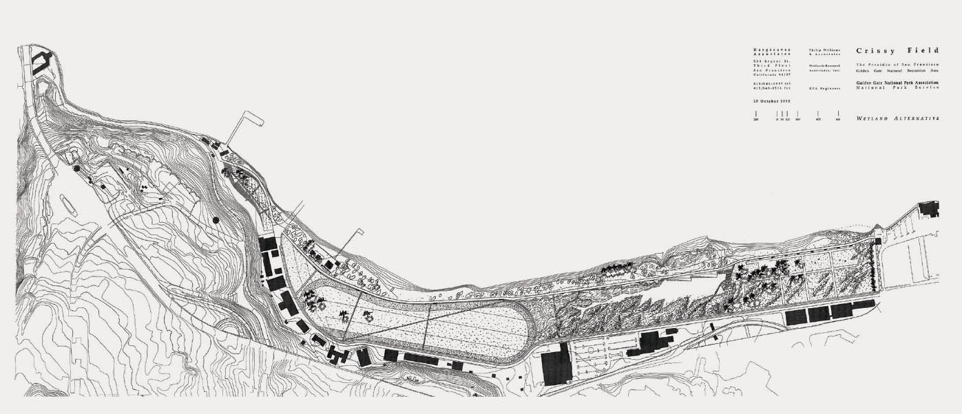
37.7833° N, 122.4167° W, Hargreaves Associates, Crissy Field, 1985.
Topographic manipulation is central to the work of Hargreaves Associates, as exemplified at Crissy Field, a linear park along San Francisco Bay. The landform design is studied in model and translated into a two-dimensional representation that emphasizes gesture, grain, and choreography. Sandwiched between the continuous contours of shoreline and upland, the designed topography provides a counter scale and orientation, directing the movement of wind and people on-site and the eye through the drawing.
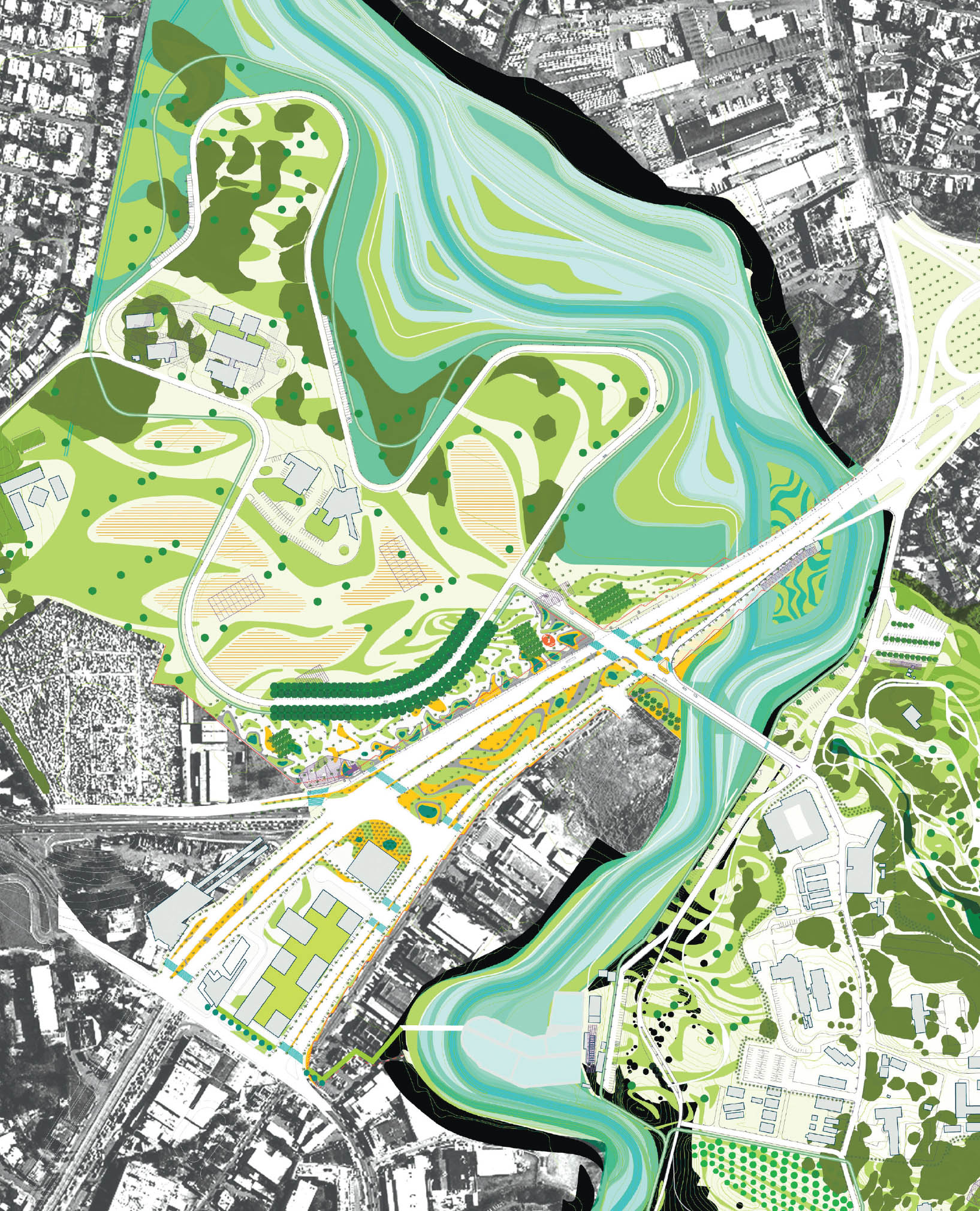
2.14
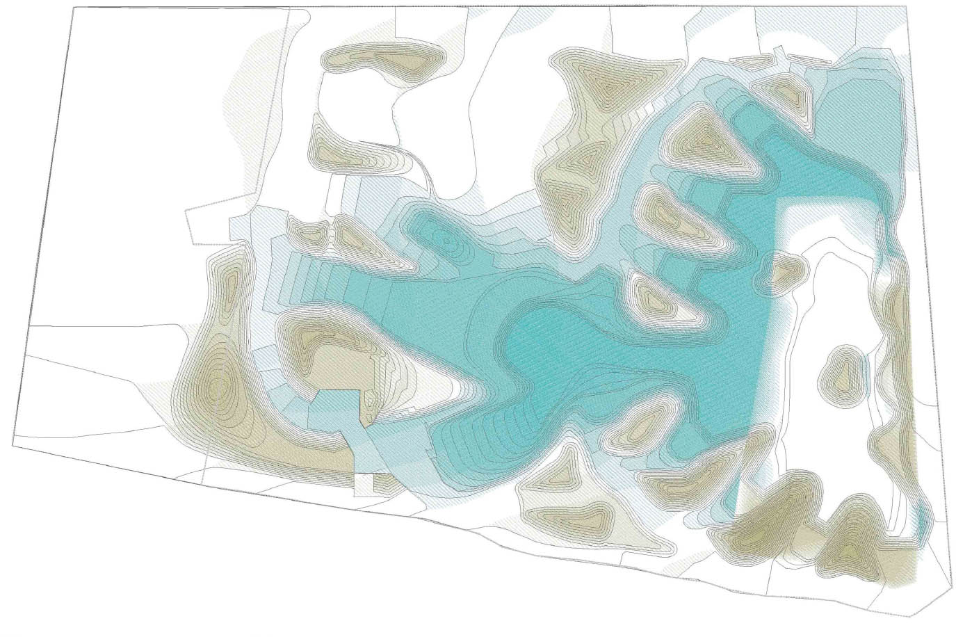
43.6481° N, 79.4042° W, OLM; Atelier Girot; ARUP; J. Mayer H. und Partner, Architekten; ReK Productions; Applied Ecological Services, TRM Toronto—Lower Don, 2007.
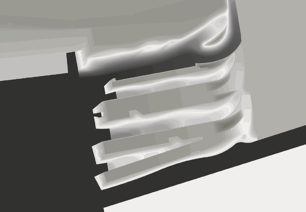
The double ramp of this hypsometric tint creates a dramatic read of the topography proposed for extension of the city fabric into the port lands at the mouth of the Don River in Toronto. Known for its landform-driven approach to design, OLM carved the water’s edge away to reintroduce lacustrine marshes and to amplify the city-water interface. The drawing further blurs the reading of the city-water boundary. The lower elevations go from darker to lighter, but the gradient repeats. The result highlights the interface between land and water—the white—and produces the effect of a glowing edge.
2.15
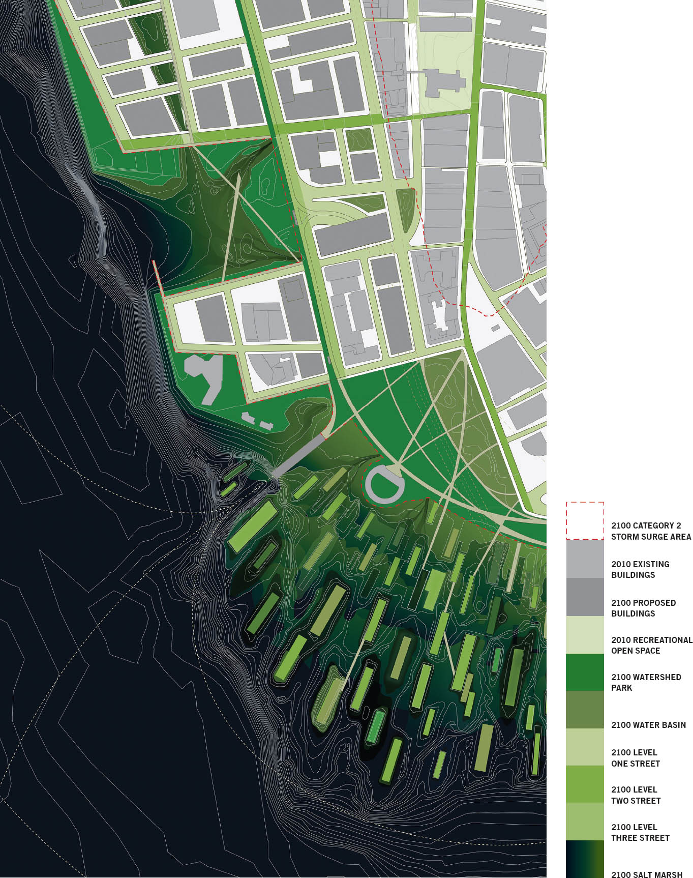
40.7697° N, 73.9735° W, Architecture Research Office (ARO) and dlandstudio, MoMA Rising Currents: Projects for New York’s Waterfront, 2010. Scale: 1:3,000 (shown at half size).
This drawing, a proposal to accommodate sea-level rise in Manhattan, shows bathymetric information as isolines and articulates the amphibious salt marsh through a color gradient from deep blue to deep green. Both color and contour index the elevation levels, representing the likelihood of flooding. Upland water capture strategies are rendered typologically with different values of green assigned to each strategy. Changes in elevation are indicated through contour alone. The subtle grading of the land-water interface is reinforced through the use of two techniques for describing terrain—line and tint—focusing the viewer on the area most susceptible to rising tides.
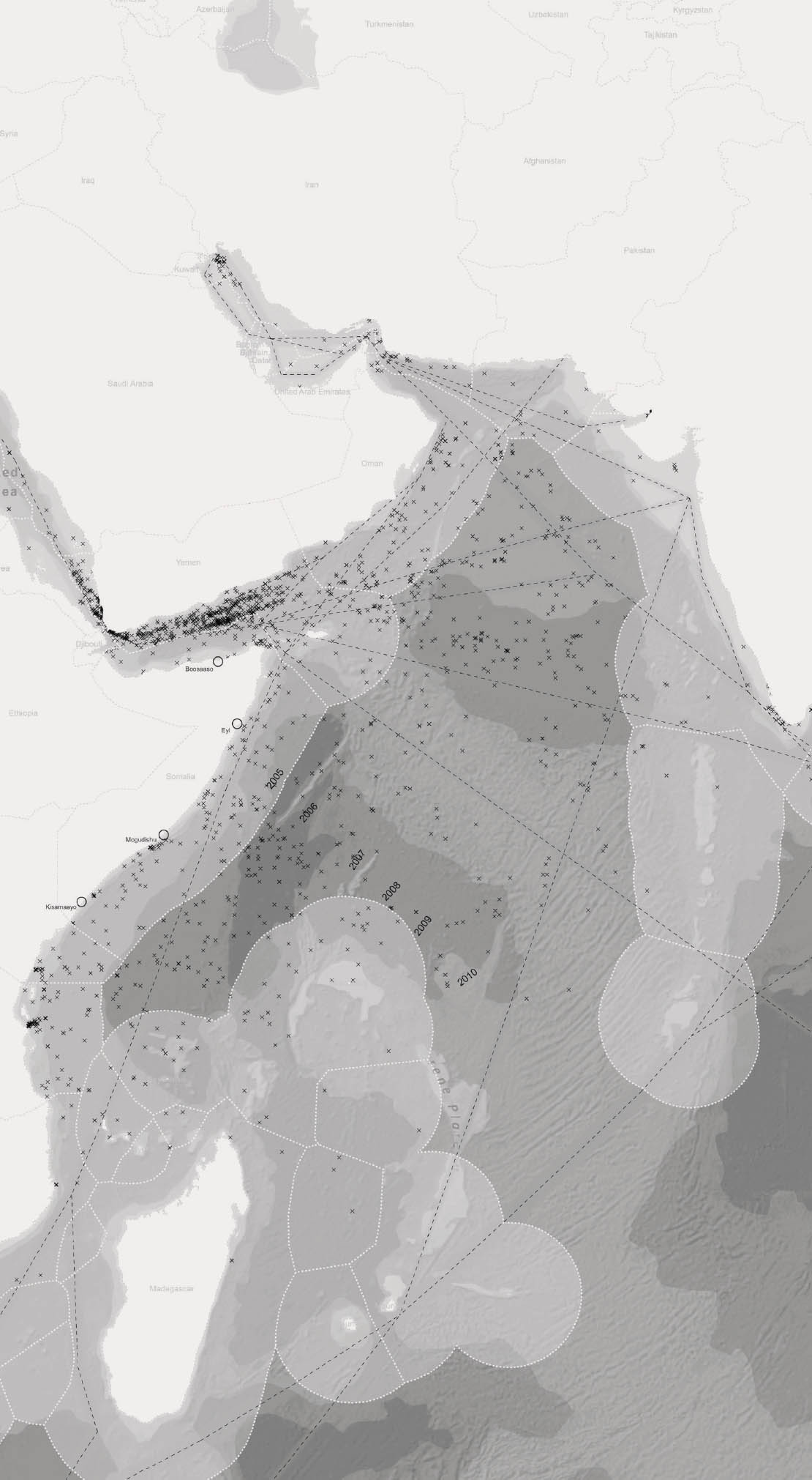
2.16
12.5458° N, 48.1456° E, OPSYS/Alexandra Gauzza, Coastal Piracy or Coast Guard?, 2012.
The map shows an increasing number of attacks along primary shipping lanes, juxtaposing incidents of coastal piracy against maritime routes off the coast of Somalia. The drawing makes visual the results of the complex social, economic, and political circumstances involved in the defense of the 3,300-kilometer coastline. The drawing, through the near omission of land information, and the transparent offset along the edges, highlights this long coast while drawing attention to water-driven activity. The ocean and its floor are richly rendered using a shaded relief to show the intricate topography and bathymetric tints to give clarity to the overall morphology.
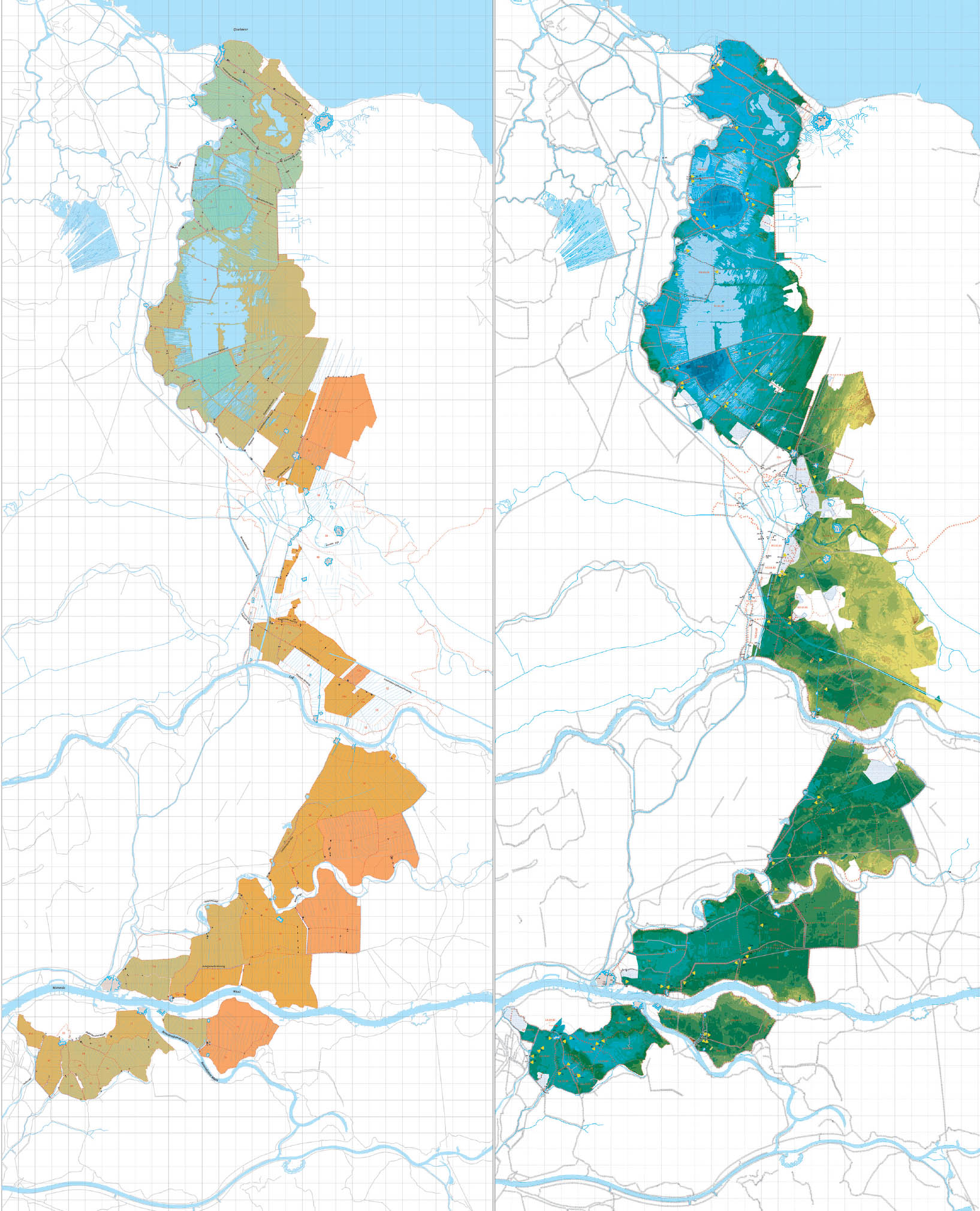
2.17
52.2066° N, 5.6422° E, Clemens Steenbergen, Johan van der Zwart, Joost Grootens, Atlas of the New Dutch Water Defence (Rotterdam: nai010 Publishers, 2009), 68, 132.
The maps contained within Atlas of the New Dutch Water Defence Line use classic cartographic techniques—color, hachures, contour, line symbols, conventional signs—in innovative ways to examine the complexity of the 135-kilometer line of fortifications encompassing the cities of Amsterdam and Utrecht through history. The first map shows the polder drainage. The second map shows the location and height of the polders within the floodplain, using tints to both describe the topographic subtleties and highlight the region under Dutch control.
2.18
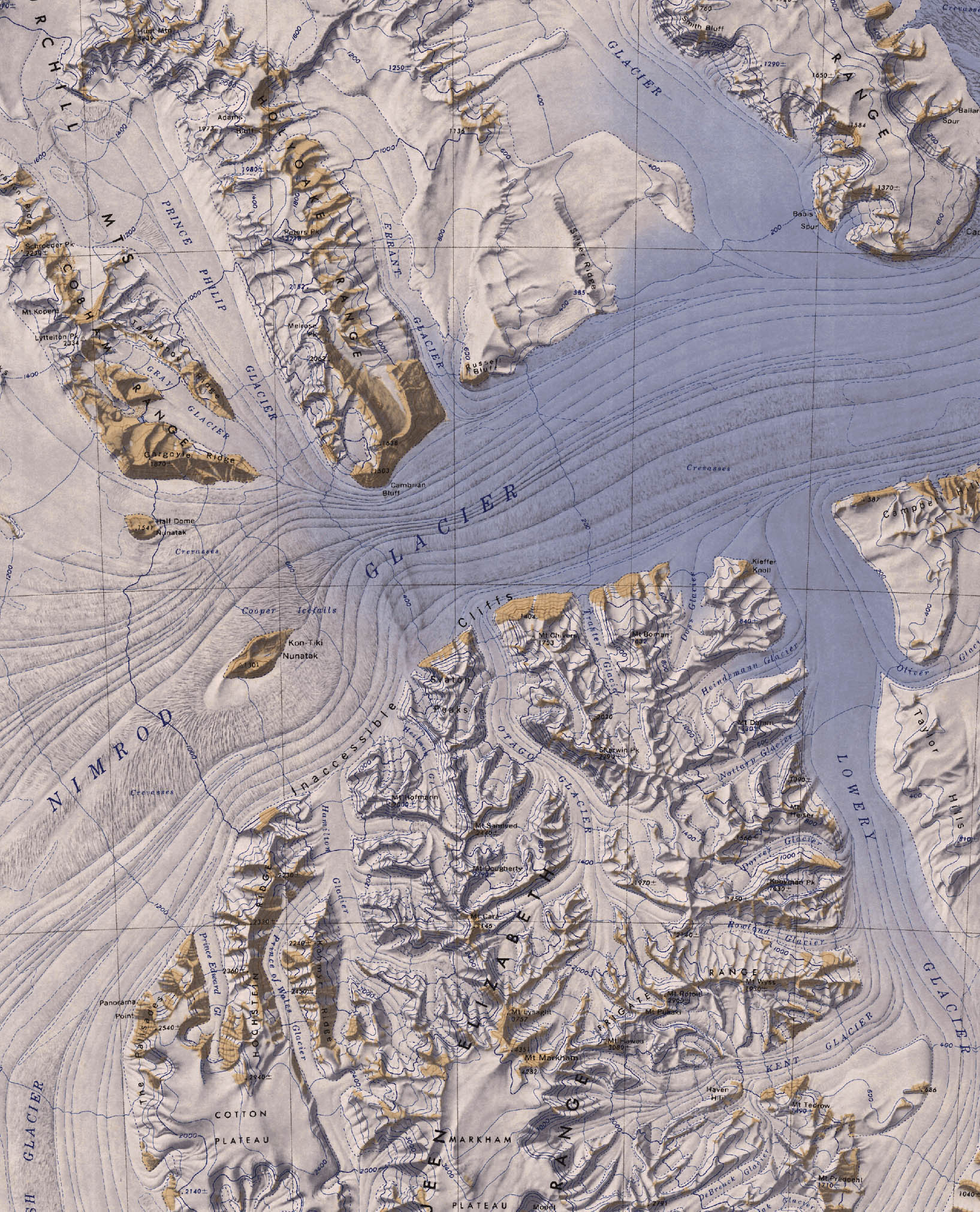
81.3500° S, 163.0000° E, United States Geological Survey (USGS), Nimrod Glacier, Topographic Reconnaissance Maps of Antarctica, 1963. Scale: 1:250,000 (shown at full size).
The USGS began sending surveyors to Antarctica annually in 1957 to work with the navy in establishing geodetic control and to gather mapping-quality aerial photography. The topographic reconnaissance maps that resulted are visually extraordinary, with a combination of terrain-rendering techniques that bring a visceral quality to a remote environment. Contours, shading, hachures, and color are all used to describe the topography and ground condition (moraine, glacier, crevasse, ice shelf, iceberg, fast ice).
2.19
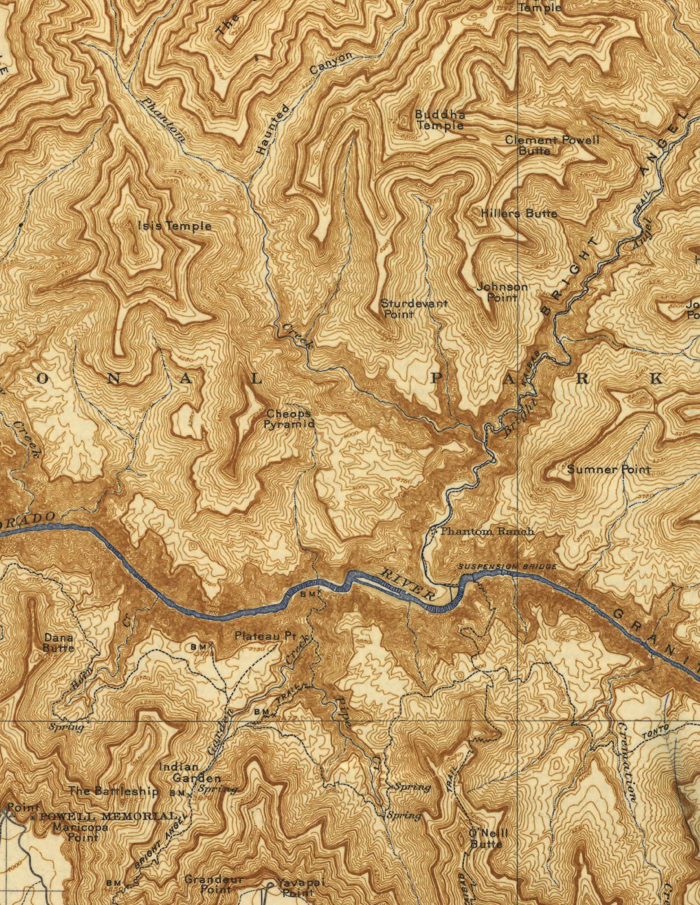
36.0574° N, 112.1428° W, USGS, Grand Canyon: Bright Angel, 1903. Scale: 1:48,000 (shown at full size).
François Emile Matthes, a renowned topographer and geologist, completed the first real survey of the Grand Canyon Bright Angel area between 1902 and 1904. His method—taking multiple sights through the transit from exceptional vantage points and then sketching the rough form of the land—resulted in beautiful sketches, refined contour lines, and new routes through the landscape. The USGS quadrangle from 1903 highlights the Matthes topography with contour alone. The simple language of the drawing allows for a focus on the landform. The steepness of the canyon—the density of lines—express the three-dimensional quality of the place without the need for further shading and texture.
2.20
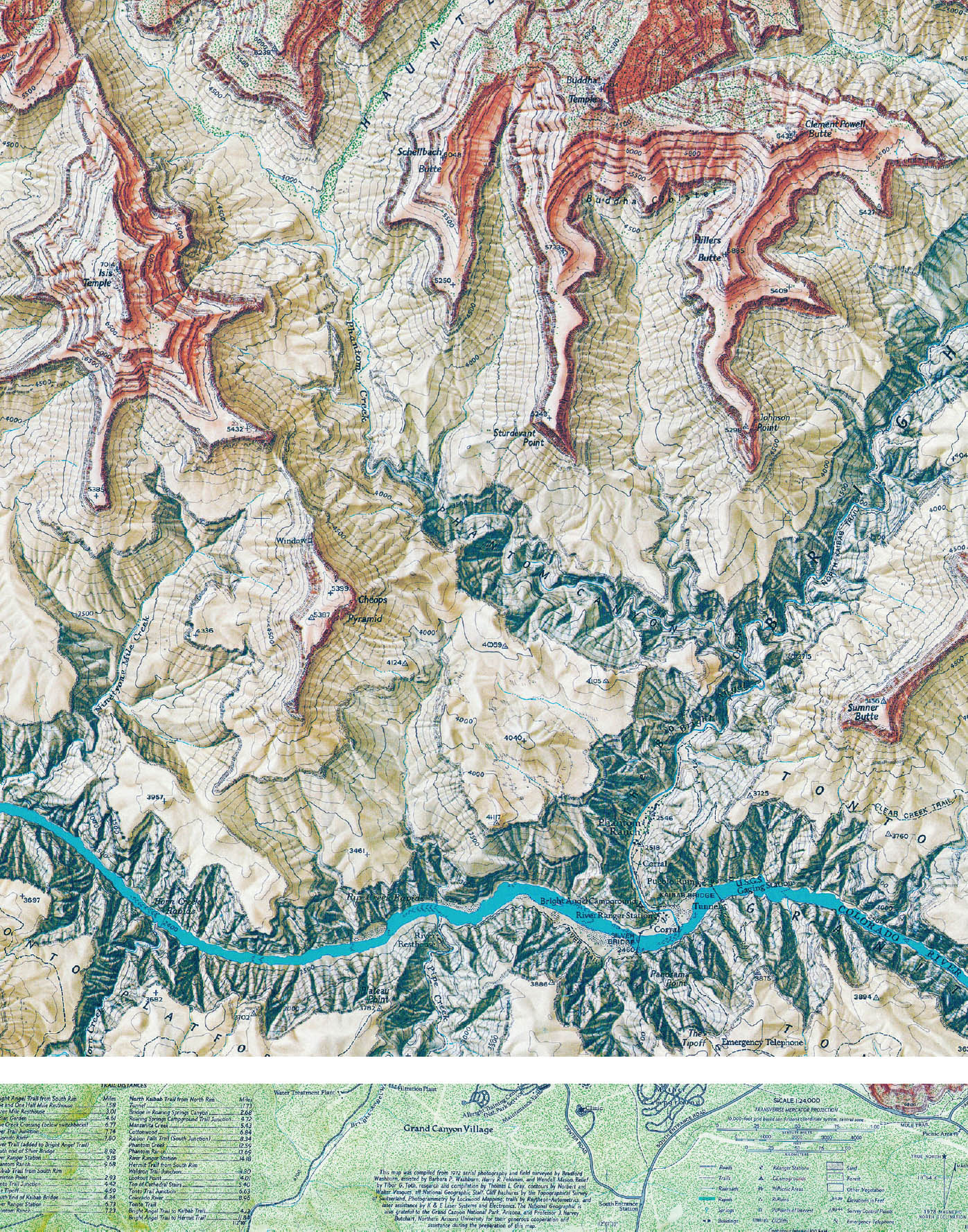
36.0574° N, 112.1428° W, William T. Peele, Richard K. Rogers, Bradford Washburn, Tibor G. Tóth, The Heart of the Grand Canyon, 1978. Scale: 1:24,000 (shown at half size).
Inspired by the work of Matthes and motivated by their own sense of cartographic adventure, Bradford and Barbara Washburn led an expedition to map the Grand Canyon in 1974. The effort focused on the 170-square-mile heartland of the canyon—the area most visited by tourists—and the same area included in the 1902–4 Matthes survey. The mapping expedition required 146 days of fieldwork spread across four and a half years. The process included extensive climbing and exploration and a recorded 695 helicopter flights, as well as a recently introduced laser beam, allowing for new degrees of precision across massive distances. The final map, a National Geographic classic, embodies incredible precision, both in its underlying survey and in its drawing technique.