A great many of the fundamental laws of the various branches of science are expressed most simply in terms of differential equations. For example, the motion of a particle of mass M, when acted upon by a force whose components along the three axes of a cartesian reference frame are Fx, Fy, and Fz, is given by the three differential equations
where x, y, z is the position of the particle at any time t. In this case the motion is given by a system of ordinary differential equations.
The physical laws governing the distribution of temperature in solids, the propagation of electricity in cables, and the distribution of velocities in moving fluids are expressed in terms of partial differential equations. It is therefore necessary that the student of applied mathematics should have a clear idea of the fundamental definitions and operations involving partial differentiation.
A quantity F(x,y,z) is said to be a function of the three variables x, y, z if the value of F is determined by the values of x, y, and z. If, for example, x, y, and z are the cartesian coordinates of a certain point in space, then F(x,y,z) may be the temperature at that point, and as x, y, and z take on other values, F(x,y,z) will give the temperature in the region under consideration.
The function F(x,y,z) is continuous at a point (a,b,c) for which it is defined if
independently of the manner in which x approaches a, y approaches b, and z approaches c.
Now, given F(x,y,z), it is possible to hold y and z constant and allow x to vary; this reduces F to a function of x only which may have a derivative defined and computed in the usual way. This derivative is called the partial derivative of F with respect to x. Therefore, by definition,
The symbol ∂F/∂x denotes the partial derivative. Sometimes the alternative notations are used:
Again, if we hold x and z constant, we make F a function of y alone whose derivative is the partial derivative of F with respect to y; this is written
In the same manner we define the partial derivative with respect to
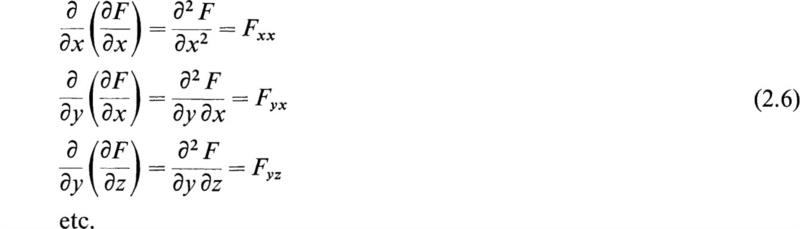
If F(x,y,z) has partial derivatives at each point of a domain, then those derivatives are themselves functions of x, y, and z and may have partial
derivatives which are called the second partial derivatives of the function F. For example,
∂2F/(∂x∂y) denotes the derivative of ∂F/∂y with respect to x, while ∂2F/(∂y∂x) denotes the derivative of ∂F/∂x with respect to y. It may be shown that if F(x,y) and its derivatives ∂F/∂x and ∂F/∂y are continuous then the order of differentiation is immaterial, and we have
In general ∂p+qF/(∂xp∂yq) signifies the result of differentiating F(x,y,z) p times with respect to x and q times with respect to y, the order of differentiation being immaterial. The extension to any number of variables is obvious.
In Appendix C, Sec. 16, we wrote Taylor’s expansion of a function of one variable in the form
where
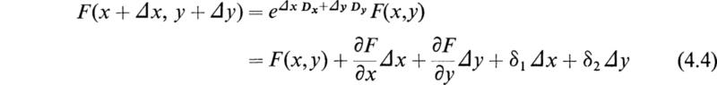
and e is the base of the natural logarithms. The symbolic expansion of a function F(x,y) of two variables written in the form
where
is to be interpreted by substituting
and operating with the result on F(x,y). Terms of the type Drx and Drx Dsy, etc., are interpreted by
The justification of (3.1) depends on the fact that the operators Dx and Dy satisfy certain laws of algebra and commute with constants, as discussed in Chap. 7. This form of Taylor’s expansion is of great usefulness in applied mathematics.
As a simple case of composite functions, let us consider
where x and y are both functions of the independent variable t, that is,
Now if t is given an increment Δt, then x and y receive increments Δx, Δy, and F receives an increment ΔF given by
Now, by Taylor’s expansion, we have
where
Hence
Dividing this by Δt and taking the limit as Δt → 0, we have
Now as Δt → 0, Δx → 0, and Δy → 0, and if t is the only independent variable, we have
Therefore, provided the functions x(t) and y(t) are differentiable, (4.7) becomes
If there are other independent variables besides t, then we must use the notation
and we have
This formula may be extended to the case where F is a function of any number of variables x, y, z, . . . and x, y; z, . . . , etc., are functions of the variables t, r, s, p,. . . , etc.
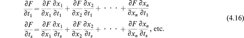
The results may be stated in the following form: If F is a function of the n variables x1 x2,. . . , xn so that
and each variable x is a function of the single variable t so that
then
If, however, each variable x is a function of the p variables t1 ,t2, . . . , tp so that
then
As an illustration of the manner in which higher derivatives may be computed from these fundamental formulas, let us differentiate (4.9) on the assumption that x and y are functions of the single variable t. We therefore have
Now since ∂F/∂x and ∂F/d∂ are functions of x and y, we apply (4.9) to ∂F/∂x and ∂F/∂y instead of to F and obtain
and
Substituting these in (4.17), we have
Expressions for the third and higher derivatives may be found in a similar manner.
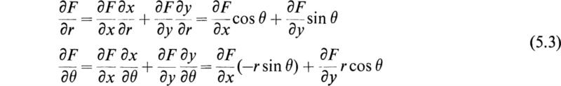
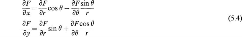
An important application of Eq. (4.11) is its use in changing variables; for example, let
and it is desired to replace x and y by the polar coordinates r and θ given by
Then F becomes a function of r and θ, and we have by (4.11)
Solving these equations for ∂F/∂x and ∂F/∂y, we have
The second derivatives may be computed by Eq. (4.20).
For simplicity, let us consider
a function of two variables x and y. Now let us give x an increment Δx and y an increment Δy. Then, as was stated in (4.6), F takes an increment ΔF, where
provided ∂F/∂x and ∂F/∂y are continuous.
In general the third term is an infinitesimal of higher order than the first term, and the fourth term is in general a higher-order infinitesimal than the second. We take the first two terms of (6.2) and call them the differential of F and write
The definition is completed by saying that if x and y are independent variables
then (6.3) takes the form
This expression is called the total differential of F(x, y). This definition may be extended to the case where F is a function of the n independent variables x1, x2, . . . , xn to obtain
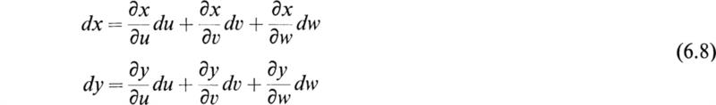
This definition (6.5) has been based on the assumption that x and y are independent variables. Let us now examine the case where this is not true. Let us suppose that x and y are functions of the three independent variables u, v, w, so that
Now since u, v, and w are independent, we have
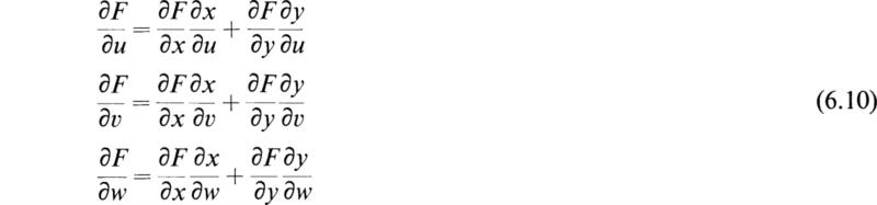
And since F is a function of u, v, and w, we have
But, by Eqs. (4.16), we have
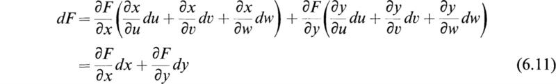
Substituting these equation into (6.9), we have
This is the same as (6.5). It thus follows that the differential of a function F of the variables x1, x2, . . . , xn has the form (6.6) whether the variables x1 ,x2, . . , xn are independent or not.
Let us now consider the case where
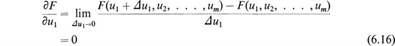
where C is a constant. This relation cannot exist when x1, x2, . . . ,xn are independent variables unless F = C. Let us suppose that x1, x2, . . . , xn are functions of independent variables u1, u2,. . . , um. Hence F may be regarded as a function of the variables u1, u2, . . . , um,, and we write
Hence
Now, since u1, u2, . . , um are independent variables, u1 may be changed without changing the value of the other variables or the value of F since F = C. Therefore
Hence
In the same manner we may prove that
Hence, as a consequence of (6.14), we have
and by (6.6) we have
If we have the relation
we are accustomed to say that this equation defines y as an implicit function of x and is equivalent to the equation
If the functional relation (7.1) is simple, then we can actually solve (7.1) to obtain y in the form (7.2). For example, consider
This equation may be solved for y to give
However, if Eq. (7.1) is complicated, it is in general not possible to solve it for y. It may be shown that y in (7.1) satisfies the definition of a function of x in the sense that when x is given (7.1) determines a value of y. It is convenient to be able to differentiate (7.1) with respect to either x or y without solving the equation explicitly for x or y.
To differentiate (7.1), let us take its first differential. As a special case of (6.19) we have
and hence
This may be written in the form
To obtain the second derivative, let
Applying (7.7) to ϕ, we have
Now
and
Substituting in (7.9), we obtain
since
![]()
Repeating this process, we may find the derivatives y‴, y″″, etc., provided the partial derivatives of F(x,y) exist and provided that ∂F/∂y ≠ 0.
The equation
defines any one of the variables, for example, x, in terms of the other two. If we take the differential of (7.13), we have
If we place y = const, then dy = 0, and we have
where the subscript denotes that y is held constant. This is less ambiguous than the notation ∂z/∂x If x = const, we have
If z = const, we obtain
Multiplying Eqs. (7.15), (7.16), and (7.17) together, we have
This is sometimes written in the form
The absurdity of using ∂x, ∂y, ∂z as symbols for differentials which may be canceled is apparent from Eq. (7.19).
Quite frequently in the application of mathematics to science it is necessary to determine the maximum or minimum values of a function of one or more variables.
Let us consider a function F of the single variable x, so that
A maximum of F(x) is a value of F(x) which is greater than those immediately preceding or immediately following, while a minimum of F(x) is a value of F(x) which is less than those immediately preceding or following. In defining and discussing maxima and minima of F(x), it is assumed that F(x) and all necessary derivatives are continuous and single-valued functions of x.
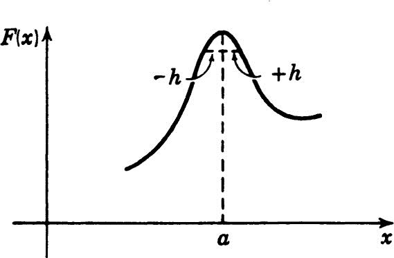
In order to determine whether the function F(x) has a maximum or a minimum at a point x = a, we may use Taylor’s expansion of a function of one variable, in the form
Let x = a be the critical point under consideration, and write
Δ(h) is thus the change in the value of the function when the argument of the function is changed by h. This is illustrated graphically, in the case that F(a) is a maximum, by Fig. 8.1.
Now, if x = a is a point at which F(x) has either a maximum or a minimum, we shall have for h sufficiently small
since for a maximum, if we move to the left of the critical point or to the right of the critical point, the function will decrease and for a minimum point the function will increase. Now if
then for h sufficiently small
since the higher-order terms in (8.3) may be neglected. In the same way
Hence, in order for (8.4) to be satisfied, we must have
at either a maximum or a minimum. Now at a maximum Δ(h) must be negative and at a minimum Δ(h) must be positive for either positive or negative values of h.
Hence, if (8.8) is satisfied, for h sufficiently small,
Since h2 is always positive, then it is evident that at a maximum we must have
and at a minimum
Fig. 8.1
Then for h sufficiently small
Since, if F‴(a) ≠ 0, the expression (8.13) changes sign with h, we cannot have a maximum or a minimum. If, however,
then for h sufficiently small
Hence F(a) will be a maximum if
and a minimum if
We define the maximum and minimum values of a function F(x, y) of two variables x, y in the following manner:
F(a,b) is a maximum of F(x,y) when, for all sufficiently small positive or negative values of h and k,
F(a,b) is a minimum of F(x, y) when, for all small positive or negative values of h and k,
By Taylor’s expansion of a function of two variables, we have, if the necessary derivatives exist and are continuous,
Letting Fx = ∂F/∂x, Fy = ∂F/∂y,
evaluated at the point x = a, y = b. Then
It is thus evident that for small values of h and k, in order for Δ(h,k) to have the same sign independently of the signs of h and k, it is necessary for the coefficients of h and k in (8.22) to vanish. This gives
evaluated at x = a, y = b as a required condition for either a maximum or a minimum. If the conditions (8.23) are satisfied, then Δ(h,k) reduces to
To facilitate the discussion, we make use of the identity
We may then write (8.24) in the form
The sign of Δ(h,k) given by (8.26) is independent of the signs of h and k provided that
or
This may be seen since (Ah + Bk)2 is always positive or zero; therefore, if AC – B2 is negative, the numerator of (8.26) will be positive when k = 0 and negative when Ah + Bk = 0.
Therefore a second condition for a maximum or a minimum of F(x, y) is that at the point in question
An investigation of the exceptional cases when (8.28) is satisfied or when
is beyond the scope of this discussion. The reader is referred to Goursat and Hedrick.† When condition (8.29) is satisfied at x = a, y = b, we see that F(a,b) will have a maximum when
evaluated at x = a, y = b. F(a,b) will have a minimum when
evaluated at x = a, y = b.
If
then F(x,y) has neither a maximum nor a minimum. By a similar course of reasoning we obtain the conditions for maxima and minima of functions of three or more variables.
As an example of the above theory, let it be required to examine
for maximum and minimum values. Here
The conditions (8.23) are
Condition (8.29) is
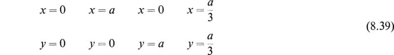
The system of Eqs. (8.37) has the four solutions
Only the last values satisfy (8.38), and a maximum or a minimum of F(x,y) is located at
If a is positive, ∂2F/∂x2 is positive when y = a/3; therefore
is a minimum. If a is negative, ∂2F/∂x2 is negative when y = a/3; hence –a3/27 is a maximum.
In a great many practical problems it is desired to find the maximum or minimum value of a function of certain variables when the variables are not independent but are connected by some given relation.
For example, let it be required to find the maximum or minimum value of the function
and let the variables x, y, and z be connected by the relation
In principle it should be possible to solve (8.43) for one variable in terms of the other two. This variable may then be eliminated by substitution into (8.42). Then the maximum or minimum values of u may be investigated by the methods discussed above since, by the elimination, u has been reduced to a function of two variables. In many cases the solution of (8.43) for any of the variables may be extremely difficult or impossible. To deal with such cases, Lagrange used an ingenious device which is known in the literature as the method of undetermined multipliers. This method will now be discussed.
If u is to have a maximum or minimum, it is necessary that
Hence
Differentiating the functional relation (8.43), we obtain
Let us now multiply (8.46) by the parameter λ and add the resulting equation to (8.45). We thus obtain
This equation will be satisfied if
The three Eqs. (8.48) and Eq. (8.43) furnish four equations to determine the proper values of the variables x, y, z and λ to assure the maximum or minimum value of the function u.
As an example of the use of this method, let it be required to find the volume of the largest parallelepiped that can be inscribed in the ellipsoid
In this case the function to be maximized is
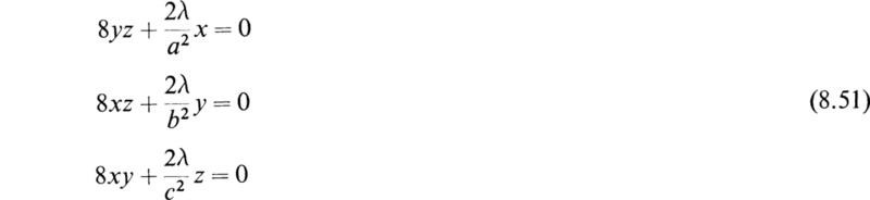
and Eqs. (8.48) are
Multiplying the first equation by x, the second one by y, and the last one by z, and adding them, we obtain
In view of (8.49) this becomes
Hence
From the first equation (8.51) multiplied by x, we have
Similarly
Hence the required maximum volume is
It is frequently required to differentiate a definite integral with respect to its limits or with respect to some parameter. Let F(x,u) be a continuous function of x, u, and consider
where u is a parameter appearing in the integrand and we assume that the limits a and b of the definite integral are continuous functions of the parameter u, so that
The integral therefore defines a function ϕ(u) of the parameter u. We shall now show that differentiation of the function ϕ(u) yields the important equation
To establish this equation, let u be given an increment Δu in (9.1).
Hence
where Δa and Δb are the increments that a and b take when u is increased by Δu. Then
Now by the concept of the definite integral of a continuous function, between the limits x1 and x2, we have
where x0 is some intermediate point between x2 and x1 given by
This may be seen intuitively by the concept of the integral (9.6) giving the area under the curve F(x) between the points x1 and x2. In this case F(x0) is a mean ordinate such that when it is multiplied by the length x2 – x1 it gives the same area as that given by the integral. We may apply Eq. (9.6) to the first integral of (9.5) and obtain
where
In the same way the last integral of (9.5) may be expressed in the form
where
Now
Hence, if we divide (9.5) by Δu, using the results (9.8), (9.10), and (9.12) and realizing that
we have
This is the required result.
In the special case that a and b are fixed, we have
If F(x) does not contain the parameter u, and
we have
In the same way, differentiating with respect to the lower limit gives
These equations are useful in evaluating certain definite integrals.
The possibility of differentiating under the integral sign leads to the converse possibility of integration. Let
where a and b are constants. Multiply by du and integrate with respect to u between u0 and u. We then have
The integrations are to be carried out first with respect to x and then with respect to u. Now let us consider
We wish to show that
Let us differentiate (10.3) with respect to u. By the results of the last section, when we carry out the differentiation on the right under the integral sign, we obtain
where the differentiation has been carried out with respect to the upper limit. Hence
But, from (10.3), we have
Hence
or
as was to be proved. This shows the possibility of interchanging the order of multiple integrations.
As an example of the use of the concept of integrating under the integral sign, consider
Now
Now multiply by du, and integrate between a and b. Then
But
Now
Hence
The evaluation of various definite integrals will illustrate some of the general principles discussed in Sec. 10. Let us consider the integral
If we change the sign of b, then the sign of the integral is changed. Placing b = 0 causes the integral to vanish. However, if we let
then we obtain
This shows that the integral does not depend on b but is a constant. Considered as a function of b, it has a discontinuity at b = 0.
Let us consider the integral
If we let k be the complex number
then we have
Separating the real and imaginary parts, we obtain the two integrals
Let us integrate (11.7) with respect to b and obtain
Placing a = 0 in (11.9), we obtain the result
The integral
occurs very frequently in many branches of applied mathematics, particularly in the theory of probability. This integral represents the area of the so-called “probability curve”
Since the indefinite integral cannot be found except by a development in series, we are led to employ a certain device to evaluate the definite integral. Since the variable of integration in a definite integral is of no importance, we have
Multiplying these integrals together, we obtain
It is permissible to introduce ![]() under the sign of integration since x and y are to be considered as independent variables. If we consider x and y as the coordinates of a cartesian reference frame and let z be a vertical coordinate, then the double integral (11.4) will represent the volume of a solid of revolution bounded by the surface
under the sign of integration since x and y are to be considered as independent variables. If we consider x and y as the coordinates of a cartesian reference frame and let z be a vertical coordinate, then the double integral (11.4) will represent the volume of a solid of revolution bounded by the surface
We may find this volume by introducing polar coordinates. Then the element of area in the xy plane is
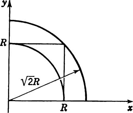
There may be some question concerning the validity of this process since the double integral (11.14) is the limit
which represents the volume over a square in the xy plane of sides equal to R (see Fig. 11.1).
Fig. 11.1
It is easy to see that this volume is greater than that of the figure of revolution over the circle of radius R and less than that over the circle of radius ![]() . Hence if the integral
. Hence if the integral
approaches a limit for R = ∞ , we have
The integration with respect to θ merely multiplies by π/2, while in the integral
the fact that we have an exact differential makes integration possible. Passing to the limit, we have
We therefore have the desired result
If in this integral we make the change in variable
then we obtain
or
To illustrate a slightly different device, let us consider the integral
This integral may be differentiated with respect to a to obtain
If we now change the variable of integration by putting
then (11.27) becomes
This is a linear differential equation with constant coefficients for I. Its general solution is
where C is an arbitrary constant to be determined. Placing a = 0, I reduces to
Therefore
Hence we have finally
The above examples illustrate typical procedures by which certain definite integrals may be evaluated.
We have seen that a necessary condition for a function F(x) to have a maximum or a minimum at a certain point is that the first derivative of the function shall vanish at that point; also a necessary condition for a maximum or a minimum of a function of several variables is that all its partial derivatives of the first order should vanish.
We now consider the following question: Given a definite integral whose integrand is a function of x, y and of the first derivatives y′ = dy/dx,
for what function y(x) is the value of this integral a maximum or a minimum? In contrast to the simple maximum or minimum problem of the differential calculus the function y(x) is not known here but is to be determined in such a way that the integral is a maximum or a minimum. In applied mathematics we meet problems of this type very frequently. A very simple example is given by the question, “What is the shortest curve that can be drawn between two given points?” In a plane, the answer is obviously a straight line. However, if the two points and their connecting curve are to lie on a given arbitrary surface, then the analytic equation of this curve, which is called a geodesic, may be found only by the solution of the above problem, which is called the fundamental problem of the calculus of variations.
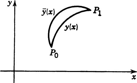
It will now be shown that the maximum or minimum problem of the calculus of variations may be reduced to the determination of the extreme value of a known function. To show this, consider functions ![]() of x that are “neighboring” functions to the required function y(x).
of x that are “neighboring” functions to the required function y(x).
The function ![]() is obtained as follows: Let
is obtained as follows: Let ![]() be a small quantity, and let n(x) be an arbitrary function of x which is continuous and whose first two derivatives are continuous in the range of integration. We then introduce into the integral (12.1) in place of y and y′ the neighboring functions
be a small quantity, and let n(x) be an arbitrary function of x which is continuous and whose first two derivatives are continuous in the range of integration. We then introduce into the integral (12.1) in place of y and y′ the neighboring functions
We stipulate, however, that these functions ![]() coincide with the function y(x) at the end points of the range of integration, as shown in Fig. 12.1. It must therefore be required that the arbitrary function n(x) vanish at the end points of the interval.
coincide with the function y(x) at the end points of the range of integration, as shown in Fig. 12.1. It must therefore be required that the arbitrary function n(x) vanish at the end points of the interval.
If we substitute the function ![]() into the integral, then the integral becomes a function of
into the integral, then the integral becomes a function of ![]() . We then require that y(x) should make the integral a maximum or a minimum; that is, the function I(
. We then require that y(x) should make the integral a maximum or a minimum; that is, the function I(![]() ) must have a maximum or minimum value for
) must have a maximum or minimum value for ![]() = 0. That is,
= 0. That is,
should be a maximum or minimum for ![]() = 0.
= 0.
This gives us a simple method of determining the extreme value of a given integral. The condition is
We expand the integrand function F in a Taylor’s series in the form
Fig. 12.1
If we differentiate (12.7) inside the integral sign with respect to ![]() , we obtain
, we obtain
This expression must vanish for ![]() = 0. Since the terms in
= 0. Since the terms in ![]() ,
, ![]() 2, . . . vanish for
2, . . . vanish for ![]() = 0,we have the condition
= 0,we have the condition
The second term of (12.9) may be transformed by integration by parts into the form
The first term vanishes since n(x) must be zero at the limits. Hence, substituting back into (12.9), we obtain
Now, since n(x) is arbitrary, the only way that the integral (12.11) can vanish is for the term in parentheses to vanish; hence we have
This equation must be satisfied by y if y is to make the integral (12.1) either a maximum or a minimum. It is known in the literature as the Euler-Lagrange differential equation.
The investigation whether this equation leads to a maximum or a minimum is difficult but is seldom necessary in applied mathematics.
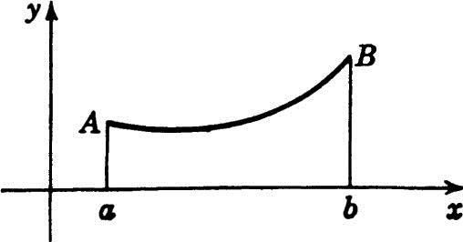
As an example of the application of Eq. (12.12), consider the problem of determining the curve between two given points A and B (cf. Fig. 12.2) which
Fig. 12.2
by revolution about the x axis generates the surface of least area. The area of the surface s is given by the equation
Here we have
Therefore Eq. (12.12) becomes
This reduces to
To integrate this equation, let
This equation then becomes
and finally we have
This is the equation of the catenary curve. The constants c1 and c2 must now be determined so that the curve (12.19) will pass through the points A and B as shown in Fig. 12.2.
This is the shape that a soap film assumes when stretched between two concentric parallel circular frames. It is obvious that, in this case, the surface s is a minimum.
The case where the function F is a function of several dependent variables yk and their derivatives is of great importance. In this case we proceed as in the case of one variable and introduce as neighboring functions
where the functions nr(x) again vanish at the limits of the integral. The integral then becomes a function of the variables ![]() 1,
1,![]() 2, . . . ,
2, . . . , ![]() k. The condition for a maximum or a minimum is
k. The condition for a maximum or a minimum is
where ![]() 1 =
1 = ![]() 2 = =
2 = = ![]() r = =
r = = ![]() k = 0.
k = 0.
It follows, therefore, that, as before, the coefficient of each of the functions n within the integral sign must vanish so that we have
We thus see that the Euler-Lagrange equations hold for each of the independent variables.
In literature the notation
for ![]() small is frequently used. δI is termed the variation of the integral. The condition that the integral have a maximum or a minimum is then expressed in the form
small is frequently used. δI is termed the variation of the integral. The condition that the integral have a maximum or a minimum is then expressed in the form
δF is called the variation of F.
Perhaps the earliest problem in the calculus of variations was proposed in 1696 by the Swiss mathematician John Bernoulli. He proposed the following problem of the brachistochrone:
It is required to determine the equation of the plane curve down which a particle acted upon by gravity alone would descend from one fixed point to another in the shortest possible time.
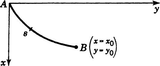
Let A be the upper point and B the lower one. Assume the x axis of a cartesian reference frame to be measured vertically downward, and let A be the origin of coordinates as shown in Fig. 12.3.
Let s be the length of the required curve at any point measured from A. Let v be the velocity of the particle at the same point and t its time of descent from A to that point. We wish to determine the curve that will make T a minimum, where T is the total time of descent from A to B. Now, from mechanics, we have
Fig. 12.3
We know that the particle loses no energy in passing from one point to another of a smooth curve, since the loss of gravitational potential energy is transformed into kinetic energy; hence
where it is assumed that the particle starts from rest and g is the acceleration due to gravity.
Therefore (12.25) becomes
and the total time T is
We must therefore minimize the integral
Hence we have
In this case the Euler-Lagrange equation becomes
Hence
where c1 is an arbitrary constant.
For simplicity, let
Squaring, clearing fractions, and transposing, we have
Hence
Therefore
Integrating, we obtain
The arbitrary constant c2 is zero since we have x = 0 at y = 0. Hence the equation of the curve is
This is the equation of a cycloid where a is the diameter of the generating circle. The constant a is determined by the condition that the cycloid must pass through the point x0, y0.
A more extended discussion of the calculus of variations is beyond the scope of this book. In recent years the application of the calculus of variations to problems of engineering and physics has proved of great value. Those interested will find the works listed in the references of this appendix.
By the extension of the principles of Sec. 12 the Euler equations that cause various integrals to attain stationary values can be obtained. The following summary of results that are useful in various applications is given here for reference.
1. One dependent variable y; one independent variable x. Integrand contains first-order derivative.
2. One dependent variable y, one independent variable x. Integrand contains derivatives y1, y2, y3,. . . , yn, where yk = dky/dxk.
3. Several dependent variables x1, x2, x3, . . . , xn, one independent variable t, first-order derivatives ![]() k = dxk/dt.
k = dxk/dt.
4. Higher derivatives, n dependent variables, one independent variable. In this case there are n Euler equations of a type similar to (13.4), one for each dependent variable.
5. One dependent variable u, two independent variables x and y.
where ux, uy are partial derivatives with respect to x and y and uxx, uyy are second partial derivatives with respect to x and y; uxy is the mixed second partial derivative with respect to x and y.
where Fu = ∂F/ ∂u, ![]() ,
, ![]() , etc.
, etc.
There are several possible formulations of the laws of mechanics. The most elementary formulation involves the concept of force and leads to the Newtonian equations which are discussed in elementary textbooks on mechanics. Another alternative and very important formulation is Hamilton’s principle. This formulation is based on the energy concept and is a very useful one, particularly in cases where Newton’s laws are difficult to apply. Hamilton’s principle assumes that the mechanical system under consideration is characterized by a kinetic-energy function T and a potential-energy function V. In the case of a mechanical system having n degrees of freedom the configuration of the system may be described in terms of the n general coordinates q1, q2, q3, . . . , qn The kinetic energy will be a function of the coordinates qk (k = 1, 2, 3, . . . , n) as well as the generalized velocities ![]() (except when the q’s are cartesian coordinates).
(except when the q’s are cartesian coordinates).
Only conservative systems will be considered in this discussion. The potential energy V will be a function of the q’s but will not depend on the velocities ![]() . We therefore have
. We therefore have
Hamilton’s principle postulates that the integral
where t1 and t2 are two instants in time, shall have a stationary value. The integrand T – V is called the Lagrangian function. Therefore Hamilton’s principle states that the motion of the dynamical system under consideration takes place in such a manner that
The integrand of (14.4) contains the n dependent variables qk and their time derivatives ![]() and the single independent variable t. The requirement that this integral be stationary leads to a system of n Euler equations of the form (13.6). These equations are
and the single independent variable t. The requirement that this integral be stationary leads to a system of n Euler equations of the form (13.6). These equations are
or
These are the Lagrangian equations of motion of the system which were deduced in Chap. 6, Sec. 5, directly from Newton’s laws without the use of the calculus of variations.
In a conservative system the sum of the potential and kinetic energy of the system is a constant c. Therefore
Hence
Hamilton’s principle states that
since the variation of a constant is zero. The integral
is called the action. As a consequence of (14.9), we have
In classical mechanics this is the celebrated principle of least action. It appears to have been first announced by De Maupertuis in 1744.†
Hamilton’s principle is very useful in obtaining the equations of motion of continuous systems. For example, consider a uniform string of mass m per unit length stretched between two supports from x = 0 to x = s under the action of a constant tension k. If the string is performing small oscillations in one plane of amplitude u(x,t), it can be shown that, if the deflection u is small, the kinetic energy T and the potential energy V of the string may be expressed in the following form:
where ut and ux denote partial derivatives with respect to t and x, respectively. Hence Hamilton’s principle states that
This is an integral of the type (13.7) with
Equation (13.8) in this case reduces to the equation
or
This is the equation of motion of the string. It is the equation for the propagation of waves in one dimension and is discussed in Chap. 12.
Problems in the calculus of variations sometimes arise that involve making one integral stationary while one or more other integrals involving the same variable and the same limits are to be kept constant. For example, the problem may be to bend a wire of fixed length so that it will enclose the maximum plane area. There are many problems of this sort. As a class they are called isoperimetric problems.
For example, let it be required to find the stationary value of the integral
provided that the integral
To solve this problem, we consider the integral
where
and μ is a parameter to be determined.
It is clear that, since the integral I1 is to remain constant, the integral I0 will be stationary if I is stationary. The Euler equation that makes I0 stationary is
The parameter μ can now be eliminated by the use of Eqs. (15.2) and (15.5). As an example, let it be required to find the shape of the plane curve that must be assumed by a wire of fixed length S0 so that it encloses the maximum area. To solve this problem, it is convenient to express the shape of the curve in plane polar coordinates. We therefore seek the curve r = r(θ) that maximizes the integral
and has a fixed length
In this case we have
This equation may be written in the form
The absolute value of the left-hand member of (15.10) will be recognized as the curvature of r(θ) expressed in polar coordinates. Hence ρ= |μ|, a constant, and the curve is a circle. The value of the parameter μ may now be determined in terms of the given fixed length S0 by the use of (15.7).
1. Find the first and second partial derivatives of the function tan–1 (x/y).
2. Show that, if u = ln(x2 + y2) + tan–1 (y/x), then ∂2 u/ ∂x2 + ∂2 u/ ∂y2 = 0.
3 Show that, if u = tan(y + ax) +![]() , then ∂2u/ ∂x2 = a2(∂2u/ ∂y2).
, then ∂2u/ ∂x2 = a2(∂2u/ ∂y2).
4. If u = F1(x +jy) + F2(x – jy), where ![]() , show that
, show that
![]()
5. If F is a function of x and y and x + y = 2eθcos ϕ, x – y = 2jeθsin ϕ, where ![]() , prove that ∂2F/ ∂θ2 + ∂2F/ ∂ϕ2 = 4xy(∂2F/∂x∂y)
, prove that ∂2F/ ∂θ2 + ∂2F/ ∂ϕ2 = 4xy(∂2F/∂x∂y)
6. Change the independent variable from x to z in

where x = ez, and show that the equation is transformed to

7. Find the maximum value of V = xyz subject to the condition that
![]()
What is the geometric interpretation of this problem ?
8. Divide 24 into three parts such that the continued product of the first, the square of the second, and the cube of the third may be a maximum.
9. Find the points on the surface xyz = a3 which are nearest the origin.
10. Show that the necessary conditions for the maximum and minimum values of ϕ(x,y), where x and y are connected by an equation F(x,y) = 0, are that x and y should satisfy the two equations F(x,y) = 0 and
![]()
11. Determine the equation of the shortest curve between two points in the xy plane.
12. Find the equation of the shortest line on the surface of a sphere, and prove that it is a great circle.
13. Show that the shortest lines on a right-circular cylinder are helices.
14. Find the equation of the shortest line on a cone of revolution.
15. Find the curve of given length between two fixed points which generates the minimum surface of revolution.
16. A cubic centimeter of brass is to be worked into a solid of revolution. It is desired to make its moment of inertia about the axis as small as possible. What shape should be given ?
17. Find the curve of length 3 that joins the points (–1, 1) and (1, 1) which, when rotated about the x axis, will give minimum area.
18. Find the surface of revolution which encloses the maximum volume for a given surface area.
19. Use Hamilton’s principle to derive the equation of motion of a particle moving in a straight line with potential energy V= 1/x, where x is the distance of the particle from some arbitrarily chosen origin.
20. Assuming that a string with fixed ends will hang in such a manner that its center of gravity has the lowest possible position, find the curve in which a string of given length will hang.
21. Prove by Hamilton’s principle that the string in Prob. 20 will hang as stated.
22. Use Hamilton’s principle to obtain the polar equations for the motion of a particle in space.
23. Find the surface of revolution which encloses the maximum volume in a given area.
24. Given a volume of homogeneous attracting gravitating matter, find the shape of the solid of revolution constituting the volume so that the attraction at a point on the axis of revolution shall be a maximum.
25. Determine the shape of a curve of given length, so chosen that the area enclosed between the curve and its chord will be a maximum.
26. Consider a vibrating membrane, like a drumhead whose position of equilibrium is in the (x,y) plane. Let u(x,y,t) be the small deflection of the membrane while it is performing oscillations. Find the potential energy V and the kinetic energy T under the assumption that the membrane is under constant tension P and has a mass m per unit area. Determine the equation of motion by Hamilton’s principle.
27. Show that, if the integrand of (12.1) does not contain x explicitly so that it takes the form
![]()
then the Euler-Lagrange equation (12.12) takes the following form: F – y(∂F/∂yx) = const. This is a very useful result that can be used when the integrand F does not depend explicitly on x.
1904. Goursat, E., and E. Hedrick: “A Course in Mathematical Analysis,” vol. I, Ginn and Company, Boston.
1911. Wilson, E. B.: “Advanced Calculus,” Ginn and Company, Boston.
1925. Bliss, G. A.: “Calculus of Variations,” The University of Chicago Press, Chicago.
1927. Forsythe, A. R.: “Calculus of Variations,” Cambridge University Press, New York.
1931. Bolza, O.: “Lectures on the Calculus of Variations,” The University of Chicago Press, Chicago; reprinted, Stechert-Hafner, Inc., New York.
1933. Osgood, W. F.: “Advanced Calculus,” Chap. 17, The Macmillan Company, New York.
1950. Fox, C.: “An Introduction to the Calculus of Variations,” Oxford University Press, New York.
1951. Polya, G., and G. Szego: “Isoperimetric Inequalities in Mathematical Physics,” Princeton University Press, Princeton, N.J.
1952. Hildebrand, F. B.: “Methods of Applied Mathematics,” Prentice-Hall, Inc., Englewood Cliffs, N.J.
1952. Weinstock, R. P.: “Calculus of Variations,” McGraw-Hill Book Company, Inc., New York.
1953. Courant, R., and D. Hilbert: “Methods of Mathematical Physics,” Interscience Publishers, Inc., New York.
1962. Akhiezer, N. I.: “The Calculus of Variations,” Blaisdell Publishing Company, New York; translated by A. H. Frink.
† Goursat and Hedrick, 1904 (see References).
† See Cornelius Lanczos, “The Variational Principles of Mechanics,” University of Toronto Press, Toronto, Canada, 1949.