CHAPTER 4
File geodatabases
LEARNING GOALS
- Import data into file geodatabases.
- Modify attribute tables and fields.
- Use Python expressions to calculate fields.
- Join tables.
- Get an introduction to SQL query criteria.
- Carry out attribute queries.
- Aggregate point data to polygon summary data.
Introduction
A database is a container for all the data of an organization, project, or other undertaking for record keeping, decision-making, analysis, or research. A file geodatabase is Esri’s simplified database for geospatial data, including feature classes and raster datasets, and for processing by single users or small groups. In terms of data format, a file geodatabase is simply a file folder with .gdb at the end of its name that contains a number of files. A .gdb is not a file extension but just part of the folder name. Processing of data in a file geodatabase is done using ArcGIS Pro’s Catalog pane, geoprocessing tools, and user interface.
For example, FoodDesertsChicago.gdb could be the name of a file geodatabase that stores spatial data for analyzing residents’ access to grocery stores in Chicago, starting with feature classes for grocery stores, streets, and population in census blocks in Chicago. The workflow for estimating the number of Chicago residents who live in food deserts (that is, live a mile or more from the nearest grocery store) would have you create additional feature classes and tables, also output and stored in FoodDesertsChicago.gdb. Chapter 9 provides the workflow and spatial analysis tools (buffers or service areas of grocery stores) for carrying out such a workflow.
Although file geodatabases have a simple format, they nevertheless are powerful spatial data containers. For example, file geodatabases have no practical limits on numbers and sizes of feature classes and raster datasets stored in them; they are optimized for data processing and storage in ArcGIS Pro, and they allow data tables to be related and joined (essential database processes).
In this chapter, you will learn about working with file geodatabases in these ways:
- Importing spatial data into file geodatabases
- Modifying data
- Joining tables
- Aggregating data on individual points to group-level data in polygons
- Querying data using attribute criteria
- Building a spatial join (which is unique to GIS)
- Using ArcGIS Pro’s Catalog pane for utility work on file geodatabases
In this chapter, you must work tutorials 4-1 through 4-3 sequentially, because tutorial 4-2 uses results from tutorial 4-1, and tutorial 4-3 uses results from tutorial 4-2.
Tutorial 4-1: Import data into a file geodatabase
When you create a new ArcGIS Pro project, the software automatically creates a file geodatabase for you as the project’s default spatial data container. In this tutorial, you’ll create a new project, and then you’ll import data from external sources into the new project’s file geodatabase.
Create a new ArcGIS Pro Project
- 1.Open ArcGIS Pro.
- 2.Under Create a new project, click Blank, and make or type the selections as shown. Ensure that you clear the Create a new folder for this project check box, because the Chapter4 folder already exists.
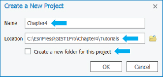
- 3.Click OK, and close the Catalog pane. ArcGIS Pro creates the new project, Chapter4.aprx, as well as a Chapter4.gdb file geodatabase and Chapter4.tbx toolbox. Next, you’ll save the project with the name Tutorial4-1, to follow the naming convention for projects in this book. Note that every new feature class, table, and other files that you create are saved by default to the project’s file geodatabase, Chapter4.gdb in this case.
- 4.On the Project tab, click Save as, and browse to the Chapter4\Tutorials folder.
- 5.For Name, type Tutorial4-1.aprx, and click Save.
- 6.Open File or Windows Explorer, and delete Chapter4.aprx from the Chapter4/Tutorials folder.
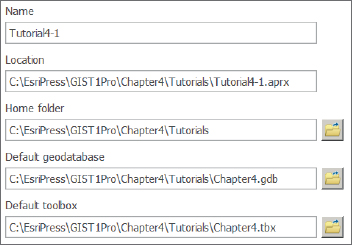
- 7.In ArcGIS Pro, on the Project tab, click Options. In the Options window on the Current Settings tab, you can see that the project, Tutorial4-1, has as its home folder Chapter4\Tutorials, and its default geodatabase is the newly created Chapter4.gdb.
- 8.Click Cancel, and click the back arrow button
 .
. - 9.On the Insert tab in the Project group, click New Map. The new map opens with the topographic basemap showing North America.
Set up a folder connection
When you created the Chapter4.aprx project (which you just renamed Tutorial4-1.aprx), ArcGIS Pro also created a folder connection to the folder in which you created the project, Chapter4\Tutorials. It’s also useful to have a connection to the Chapter4 folder because it has the Data folder within it (Chapter4\Data), which has shapefiles and other spatial data that you’ll need to access conveniently (without browsing from C:\ to C:\EsriPress to C:\EsriPress\GIST1 and to C:\EsriPress\GIST1\Chapter4). You will create connections in the Catalog pane.
- 1.Open the Catalog pane.
- 2.Expand Folders > Tutorials. Here, you will see the contents of the Tutorials folder except for the project files (such as Tutorial4-1.prx). When you need to add data in the future, you can click the Tutorials folder and have direct access to its Chapter4.gdb file geodatabase instead of having to browse along the path C:\ EsriPress\GIST1\Chapter4.
- 3.Right-click Folders, and click Add Folder Connection.
- 4.Browse to EsriPress\GIST1Pro, click the Chapter4 folder, and click OK. ArcGIS Pro adds the Chapter4 folder connection.
- 5.In the Catalog pane, expand the Chapter4 folder. Here, you will see that Chapter4 has three subfolders: Tutorials, Assignments, and Data. Now, if you need data from the Data folder, you can click Folders and click the Chapter4 connection to get quick access to it.
- 6.Hide the Catalog pane.
Import shapefiles and a data table into a file geodatabase
A shapefile is an Esri spatial data format, dating to the 1990s, for a single map layer. Although no longer Esri’s preferred spatial data format, shapefiles are still used by many spatial data suppliers. For example, the US Census Bureau is the source of shapefiles used in this exercise. You will learn more about shapefiles and other spatial data formats in chapter 5, but for now, understand that ArcGIS Pro allows you to import shapefiles and other map layer formats into file geodatabases. When stored in a file geodatabase, a map layer is called a “feature class.” When displayed as part of a map, it’s a “map layer.”
- 1.On the Analysis tab, click Tools, and in the Geoprocessing pane, search for and open the Feature Class to Feature Class tool. For inputs, this tool can use a feature class from a file geodatabase, a shapefile, or a coverage (one of Esri’s earliest spatial data formats). For outputs, the tool can copy a feature class to a different file geodatabase, convert a feature class into a shapefile, convert a shapefile or coverage into a feature class, or convert a coverage into a shapefile.
- 2.For Input Features, click the Browse button.
- 3.In the Input Features window under Project, click Folders, double-click the Chapter4 connection, click the Data folder, click the MaricopaCounty folder, select tl_2010_04013cousub10.shp, and click OK.
- 4.For Output Feature Class, type Cities. The input shapefile, for county subdivisions (cities, towns, and so on), was downloaded from census.gov, as was tl_2010_04013_cousub10.shp (census tracts). The new feature class, Cities, is automatically stored in the default file geodatabase, Chapter4.gdb.
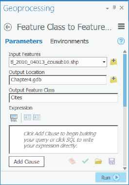
- 5.Click Run, and when the run finishes, close the tool. The imported feature class is automatically added to your map as the Cities map layer.
- 6.Open the Catalog pane, and expand Databases > Chapter4.gdb to see that the feature class, Cities, was created.
- 7.On the Catalog pane, click the Auto Hide button
 , and then click the Auto Hide button again to hide. You can now click the Project button to unhide the Catalog pane when needed.
YOUR TURN
Import shapefile tl_2010_04013.tract10.shp from Chapter4\Data\MaricopaCounty to create the feature class, Tracts, in Chapter4.gdb. Close the Geoprocessing pane when finished. Save your project.
Import a data table into a file geodatabase
Next, you’ll import a data table with some 2010 census tract data for Maricopa County. The table is in a common format for data sharing, comma-separated values, or CSV file (.csv). The first row of the table has attribute names, and subsequent rows have data with values separated by commas to delineate columns. A nonprinting line-feed character is at the end of each row, signaling the end of the row. The figure shows some rows of the table you are about to import, where GEOid is the Census Bureau’s ID number for census tracts, and the other attributes are census data. Note that if the table you want to import is in a Microsoft Excel workbook, you can save the table as a CSV file, and then import that version of the table. Comma-separated values data has the advantage of being easily imported into ArcGIS Pro; whereas, depending on how your computer is set up, Excel workbook tables may not be recognized by ArcGIS Pro.

- 1.Search for and open the Table to Table tool.
- 2.For Input Rows, browse to Chapter4\Data\MaricopaCounty, select CensusData.csv, and click OK. For Output Table type CensusData.
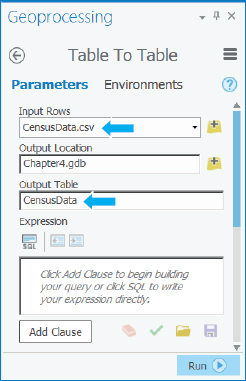
- 3.Click Run.
- 4.Close the Geoprocessing pane, and save your project.
Use database utilities of the Catalog pane
You can create, copy, rename, and delete file geodatabases in the Catalog pane. You can do the same with feature classes and tables. Suppose that you’d like to share the Tracts feature class and CensusData table with others. Next, you’ll create a new file geodatabase for sharing, copy the spatial data you want to share to it, and rename the feature class and table.
- 1.Click the Project button to open the Catalog pane.
- 2.Expand Databases to see Chapter4.gdb.
- 3.Right-click Databases, and click New File Geodatabase, and browse to open the Chapter4\Tutorials folder.
- 4.For Name, type MaricopaTracts, and click Save. MaricopaTracts.gdb is added to Databases.
- 5.Expand Chapter4.gdb, right-click its Tracts feature class, and click Copy.
- 6.Right-click MaricopaTracts.gdb, click Paste, and expand MaricopaTracts.gdb. You can see that MaricopaTracts now has a copy of the Tracts feature class.
- 7.Copy the CensusData table from Chapter4.gdb to MaricopaTracts.gdb.
- 8.In MaricopaTracts.gdb, right-click CensusData, and rename it TractsIncomeData. Now, you have just the tracts feature class and corresponding data table repackaged in the MaricopaTracts.gdb file geodatabase, which you could share with others. You don’t need this file geodatabase for any further processing in this chapter, so next you’ll delete it.
- 9.In the Catalog pane, right-click MaricopaTracts.gdb, and click Delete > Yes.
Tutorial 4-2: Modifying an attribute table
Much of what gets processed or displayed in a GIS depends on attributes—columns in tables. To get tables in the desired form, you must know how to delete, create, and modify attributes.
Get started
- 1.Save your Tutorial4-1 project as Tutorial4-2 in Chapter4\Tutorials.
- 2.Right-click Tracts, and click Zoom to layer.
- 3.Create a bookmark named Maricopa County.
- 4.Symbolize Tracts and Cities with no color and Cities with a wider and darker gray outline than Tracts.
- 5.Change the basemap to Light Gray Canvas, and then remove the World Light Gray reference layer from the Contents pane.
Delete unneeded columns
Many feature classes have extra or unnecessary attributes from the user’s point of view that you do not need and can delete.
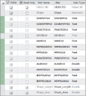
- 1.In the Contents pane, right-click Tracts, and click Design > Fields. This view allows you to modify and create attributes in a table. You cannot delete the primary key, ObjectID, or the Shape, Shape_Length, and Shape_Area attributes because they are essential. These fields are dimmed, meaning that you can’t modify them. GeoID10 is the tract geocode that you need later in this chapter for joining the CensusData table to the tracts map layer, but all other fields are candidates for deletion for the purposes of this chapter.
- 2.One group at a time, press and hold the Shift key, and select rows crossed out in the figure by clicking the first and then the last row in the group, and then right-click within a group, and click Delete. ArcGIS Pro crosses out the fields but does not delete them until you click Save. Review selections for deletion before actually deleting. If you decide to keep any of these fields, you can right-click and click Restore deleted item.
- 3.On the Fields tab, click Save.
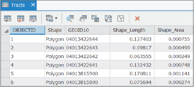
- 4.Close Fields design, and examine the Tracts table. Only the needed fields remain.
YOUR TURN
Delete all fields from Cities except for the dimmed fields, GEOID10, and Name10. Type City for Name10’s alias. Open this map layer’s table and see the remaining fields and the alias for Name10.
Examine geocodes in tables to be joined
In the next exercise, your work will prepare for joining a data table (CensusData) to the attribute table of the Tracts feature class on a one-to-one basis: each row or record in the table has one and only one matching record in Tracts. Joining two one-to-one tables makes a wider table (increases the number of columns) while leaving the number of rows the same, and is common in GIS. Joining two tables together requires each table to have an attribute with the matching values stored as the same data type (for example, numeric or text). For census tract data, the matching values are in census tract geocodes, GEOID10 in Tracts and GEOid in CensusData.
Joining tables involving census data makes sense because it is impractical to store the thousands of census tract attributes in the Tracts attribute table. The attribute table for Tracts, as downloaded from the Census Bureau’s website, has just the tract geocode and a few GIS attributes and no census data. To map census data, you will select the variables you need from the Census Bureau website (see chapter 5), download a corresponding table (which includes tract geocodes), and join the table to the tracts attribute table.
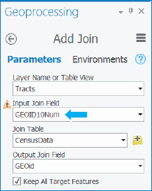
The geocodes in CensusData and Tracts would match one to one, except that GEOID10 in Tracts has a text data type whereas GEOid in Census Data has a numeric data type (as downloaded). The remedy is to create a new attribute in Tracts, say GEOID10Num, that is numeric and has the values of GEOID10 transformed from text to numbers. Tract geocodes that are text can have leading zeros dropped when converted to numeric data format. Because GEOid is numeric, it has leading zeros dropped, so the only recourse for getting matching values is to drop leading zeros in GEOID10 as well by converting it from text to numeric.
- 1.In the Contents pane, right-click CensusData, and click Design > Fields. You can see that GEOid has a numeric data type, Double (15 digits in length).
- 2.Close the CensusData Fields design view, and open the Tracts Fields design view. GEOID10 has the Text data type.
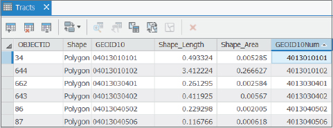
- 3.Close the Tracts Fields design view, open Tracts’s attribute table to see data values, and sort GEOID10 ascending. The first row’s value for GEOID10 has the text value 04013010101. CensusData has a corresponding numeric value, 4013010101, without the leading zero. If you created a new text attribute in CensusData, named GEOidText, its corresponding value would remain 4013010101, without the leading zero. You could add the leading zero, but it would be complicated. It is easier to create a new numeric attribute in Tracts that automatically drops any leading zeros. Then you’ll have geocodes that match.
Create a new attribute and populate it using the Calculate Field tool
Next, you’ll create the new numeric attribute in the Tracts table, and then use the Calculate Field tool to transform and copy data to it.
- 1.With the Tracts attribute table open, click its Option button and select Fields view.
- 2.At the bottom of the Fields view, click “Click here to add a new field.”
- 3.Type GEOID10Num for the Field name, and select Double as its data type.
- 4.On the Fields tab, click Save.
- 5.Close the Fields view. Notice that the values for GEOID10Num are <Null>, which signifies that data cells are empty and no data has been added as yet. These values are called “null values.”
- 6.Right-click GEOID10Num in the Tracts table, and click Calculate Field.
- 7.In the Fields pane, double-click GEOID10 in the Fields panel to create the expression GEOID10Num = !GEOID10!. The expression’s syntax is from the Python programming language, requiring attribute names on the right side to be identified using the exclamation point delimiters.
- 8.Click Run.
- 9.Close the Geoprocessing pane, and take a look at the results. The new attribute, GEOID10Num, has GEOID10 values transformed to numeric format without the leading zeros, and will match perfectly with the geocode in CensusData.
- 10.Close the Tracts table and the Geoprocessing pane.
YOUR TURN
Next, you’ll use data in the CensusData table to make a choropleth map for Maricopa County that compares incomes of Hispanics to those of whites. The CensusData table has population and per capita income for the total population, whites, Native Americans, and Hispanics. Desired for mapping are two ratios of per capita income for Hispanics and Native Americans divided by per capita income for whites. To get started, create two new attributes in the CensusData table, RatioHispanicWhiteIncome and RatioNativeWhiteIncome, both with the Float data type. When finished, close the Fields design view.
Calculate the ratio of two fields
When you calculate ratios, ensure that you do not divide by zero, which is an undefined operation in mathematics. In ArcGIS Pro, you can select rows in which the divisor is not zero, and then the Calculate Field tool will include only the selected rows, thus avoiding division by zero.
- 1.Open the CensusData table.
- 2.On the Map tab in the Selection group, click the Select By Attributes button
 .
.
Next, you’ll create the condition needed for selecting table rows in which the divisor, WhtPCIncome, is greater than 0. In tutorial 4-4, you’ll learn a lot more about attribute queries.
- 3.In the Geoprocessing pane, click Add Clause, and make the selections as shown. You can click the Values button, drop the list below it to display all existing values in the WhtPCIncome field, and then click a value (such as the zero needed here) to complete the query criterion expression. Using the drop list has the advantage of correctly formatting data values for use in queries, which works well for date and text attributes.

- 4.Click Add, and then click Run. ArcGIS Pro selects 908 out of 913 tracts, all with positive values for WhtPCIncome.
- 5.Close the Geoprocessing pane.
- 6.Right-click the heading for the RatioNativeWhiteIncome field, and click the Calculate field.
- 7.Create the expression as seen in the figure by double-clicking fields and clicking the division operator.
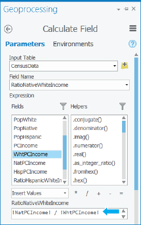
- 8.Click Run. If you get an error message, it’s likely because you don’t have records selected with nonzero WhtPCIncome.
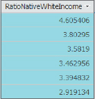
- 9.In the table, right-click RatioNativeWhiteIncome, and click Sort Descending. The figure has the results for a half dozen sorted rows sorted by RatioNativeWhiteIncome. In some tracts, Native American income is more than four times higher than whites, but in most tracts, the ratios are less than 1.
YOUR TURN
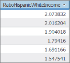
With the 908 rows of CensusData with positive WhtPCIncome still selected, create and run the following expression:

Clear the selection, close the table, and close the Geoprocessing pane when finished. Save your project. In the figure, you will see the first half-dozen records, sorted descending for the results.
Extract substring fields and concatenate string fields
If you sort the Tracts attribute table ascending for GEOID10, the first value is 04013010101. This unique identifier for a census tract is composed of three parts:
- 04 is the ANSI (American National Standards Institute) code for Arizona,
- 013 is the ANSI code for Maricopa County, and
- 010101 is the ANSI identifier for a census tract.
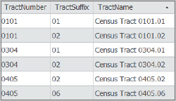
The census tract is further broken down to tract number—(the first four digits (0101) and an optional two-digit suffix (01) with an implied decimal point between the number and suffix. Formally written, the corresponding census tract name for Maricopa County, Arizona, is Census Tract 0101.01. Using GEOID10 as the input, in this exercise you’ll compute this formal representation of tracts.
- 1.In the Tracts attribute table, create three new text fields: TractNumber (length = 4), TractSuffix (length = 2), and TractName (Length = 20).
- 2.Calculate the TractNumber field with the expression
 . To understand the confusing Python language syntax of this expression, consider the case of tract 04013123456. The characters stored (digits, in this case) of any field are indexed 0, 1, 2, …, from left to right, so the positions of the 04 for Arizona are 0 and 1. The notation [0:2] extracts the indexed first digit and up to but not including the third digit, “0,” So 04 is extracted. For the case of extracting TractNumber and the example of 04013123456, the 5 of !GEOID10![5:9] corresponds to the sixth position (1) and the 9 to the 10th position (5), which is not included. So [5:9] extracts 1234.
 - 3.Calculate the TractSuffix field with the expression
 . This expression extracts the ninth digit up to but not including the 11th character, 01.
 - 4.Finally, calculate TractName with the expression:

Note that there is a space after Census Tract and before the closing double quote mark. The plus sign (+) concatenates or combines two text values into one. “Census Tract” and “ . ” in double quote marks are constants, the same for every row of data. !TractNumber! and !TractSuffix! with exclamation point delimiters denote field names, which vary by row. Sorted ascending by TractName, the figure shows the first six finished values.
YOUR TURN
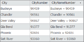
An example value for GEOID10 in the Cities attribute table is 0401390459. The first two digits are the state, the next three digits are the county, and the remaining five digits are the city. Create two new text attributes, CityNumber (length = 5) and CityNameNumber (length = 50), in the Cities attribute table. Extract the last five digits of GEOID10 in CityNumber, and then concatenate the City field and CityNumber to compute values for CityNameNumber, such as Buckeye = 90459. Put a space on both sides of the equals sign. Sorted ascending by CityNameNumber, sample values are shown next.
Tutorial 4-3: Joining tables
The next table join you will do adds the columns of the CensusData table to the attribute table of Tracts by matching values of GEOid from the CensusData table to GEOID10Num of Tracts. In this one-to-one join, each record of both tables finds a single matching record.
Each time you open a project with a table join, the join is re-created on the fly. To make a permanent Tracts and Census Data table join, you can export the Tracts feature class to a new feature class. Then the joined attributes are permanent in the new feature class. If you want to publish a feature class with a table join in ArcGIS Online, you must make the join permanent.
Get started
- 1.Save your Tutorial4-2 project as Tutorial4-3 in Chapter4\Tutorials.
- 2.Use the Maricopa County bookmark.
Join a data table to a feature class attribute table
Next, you will join the CensusData table to the Tracts feature class.
- 1.In the Contents pane, right-click Tracts, and click Joins and relates > Add Join.
- 2.In the Geoprocessing pane, make the selections as shown (ignore the warning message).
- 3.Click Run, and when the tool finishes, close the Geoprocessing pane.
- 4.Open the Tracts attribute table, scroll to the right in the table, and verify that ArcGIS Pro joined the CensusData table to the Attributes of Tracts table.
- 5.Close the Tracts table.
Export a feature class to make a join permanent
This exercise turns the join attributes of CensusData into permanent attributes of the Tracts attribute table by exporting the Tracts feature class. Also, you’ll clean up the attributes of the exported feature class.
- 1.In the Contents pane, right-click Tracts, and click Data > Export Features.
- 2.In the Geoprocessing pane, change the Output feature class’s name from Tracts_CopyFeatures to MaricopaIncome, and click Run.
- 3.Close the Geoprocessing pane.
- 4.Remove Tracts from the Contents pane.
- 5.Open the Field design view of MaricopaIncome. Notice that ArcGIS Pro has qualified each field name with its source table’s name as a prefix.
YOUR TURN
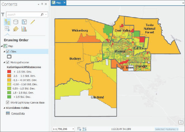
Delete these fields from the MaricopaIncome attribute table: Tracts_GEOID10, CensusData_ObjectID, and CensusData_GEOid. Edit field names to delete table name prefixes (for example, edit Tracts_GeoID10Num to GeoID10Num). Delete the Field Name prefixes, Tracts_ and CensusData_, from each field. Note that to change field names for the two ratio fields, copy and paste from the Alias column or type, which is necessary for long names. Now you can answer the question: Are there places in Maricopa County where Hispanics typically have higher per capita income than whites? Symbolize MaricopaIncome with graduated colors for symbology, RatioHispanicWhiteIncome as the field, Standard deviation for method, 1 standard deviation for interval size, and red to green for color scheme. Label and move Cities to the top of the Contents pane. You can see many places throughout Phoenix and Chandler where Hispanics earn more than whites. The tracts that have a white color are the ones for which no data was available on income for Hispanics. Save your project.
Tutorial 4-4: Attribute queries
One of the major innovations of GIS technology nearly 50 years ago was linking tabular data to the graphic features in feature classes. This linkage makes it easy to symbolize maps using the attribute values found in tables and also allows attribute queries to show only features of interest.
Attribute queries are based on structured query language (SQL), the de facto standard query language of database packages and many application software packages, including ArcGIS Pro. This tutorial introduces the query criteria part of SQL. For further study and to learn full SQL commands, you can find free interactive SQL tutorials on the Internet. A good one is at w3schools.com. The next two tutorials use crime data and queries commonly made by police crime analysts. The example queries ask some of the standard query questions of “who,” “what,” “where,” “when,” and “how.”
A simple SQL criterion has this form:

“Attribute name” is any attribute column heading or field name in an attribute table. Several logical operators are available, including the familiar ones such as =, >, >=, <, and <=. “Attribute value” is related to the values you seek. For example, this simple criterion selects all crimes that are robberies where Robbery is a value of the Crime attribute:

Text values, such as Robbery, must be enclosed in single or double quote marks.
You can use queries to select points in a feature class or set the definition query properties of a feature class. A point that is selected appears highlighted in the selection color, both in the attribute table and on the map, and all points of the map layer remain visible. A definition query, on the other hand, displays only the points that satisfy the query criteria (and without the need for highlighting).
Compound criteria are made up of two or more simple criteria connected with either an AND or an OR connector. AND means that both connected simple criteria must be true for corresponding features (records) to be selected. For example, for SQL to select features for the compound query,

the DateOccur values must be greater than or equal to August 1, 2016, and less than or equal to August 28, 2016. SQL will select a feature with the date August 5, 2016, for example, but it will exclude August 31, 2016. The date values in the criteria are in the format ArcGIS Pro requires for use in queries. You don’t have to remember such formats because the ArcGIS Pro query builder helps you get the values (and in the right format) you need in queries, as you will see in the next tutorial.
The OR connector is used to select a subset of features on the basis of classification, such as crime types in the Crime attribute. Although a single criminal incident may have one or more criminal offenses (for example, homicide and robbery in which a person was robbed and murdered), data reported by police departments to the FBI have only the most serious offense reported (homicide, in this case), so each crime has only one reported crime type. To query this kind of data for homicides and aggravated assaults, you might simply say, “I want all homicides and aggravated assaults,” but in SQL, the expression is “homicides OR aggravated assaults.” Given FBI reporting practices, it is impossible for an offense to be both a homicide and an aggravated assault because only one crime type is recorded for each offense. So, the proper SQL criteria in this case are:

Despite occasional exceptions to this rule, you will almost always need to place OR in parentheses (as shown) if the criteria are combined with other criteria, such as a date range:

The use of parentheses (just as with algebraic expressions) is because logical expressions are executed one pair at a time for simple expressions, generally working from left to right but with certain logical operators going first. For example, SQL executes AND comparisons before OR comparisons regardless of order, which can result in incorrect information unless you use parentheses to control the order of execution. SQL executes comparisons in parentheses first. For example, if you leave the parentheses out of the previous query, you’d retrieve all homicides in August 2015 but also all aggravated assaults in the database regardless of the month. Checking input data and the output results will give you experience and guidance in making compound queries.
Police need three primary kinds of attribute queries to analyze crimes, and you can combine and use these queries creatively in these ways:
- The most fundamental attribute query is by crime type and data interval (the what and when). Such queries often combine several crime types with the use of logical operators.
- The second type of attribute query adds criteria, such as time of day or day of the week—for example, weekday versus weekend crime (a refinement of when). Clearly, crime patterns can differ as a result of the time of day or the day of the week.
- The third type of attribute query adds criteria based on the attributes of the people (the who) or the objects (the what), such as vehicles, involved in a crime and can include modus operandi attributes (the how), such as “Enters through an open window,” if available.
Open the Tutorial 4-4 project
- 1.Open Tutorial4-4 in Chapter4\Tutorials, and save it as Tutorial4-4YourName.
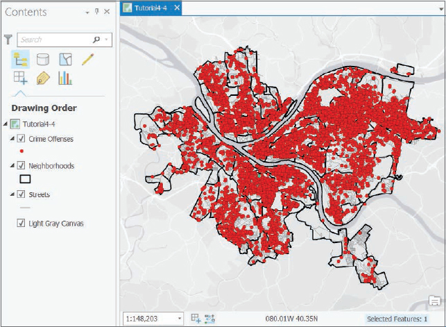
- 2.Use the Pittsburgh bookmark. The map of Pittsburgh has Crime Offenses, which has all criminal offenses for June through August 2015, Streets, and Neighborhoods. Note that the crime data, although real, has been modified to protect privacy, including changing the year of crimes. Also note that Pittsburgh is a relatively low-crime city, and that crime data plotted in any city would likely look similar to the crime data you will plot in this tutorial.
Create a date-range selection query
Queries for event locations, such as crimes, almost always use date-range criteria. A selection by attributes identifies the subset of features in a map layer that meet the query criteria and gets the selection color both in the table and on the map. Once you select the features, you can do additional processing of selected outputs. For example, you could export the selected features to a new feature class.
- 1.On the Map tab in the Selection group, click Select By Attributes.
- 2.In the Geoprocessing pane, for Layer Name, select Crime Offenses, click Add Clause, and make the selections as shown.
- Ensure that you click in the cell with the date, and select the date from the drop list.

- 3.Click Add and the Verify button
 . The Verify button ensures that there are no syntax errors but does not check for logic errors.
 - 4.Click Add Clause and make the selections as shown.

- 5.Click Add and the Verify button.
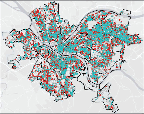
- 6.Click Run, and leave the Geoprocessing pane open. All crime offenses remain on the map, but the points for July 2015 are now displayed in the selection color. Next, you’ll save the query so that it can be reused.
- 7.In the Geoprocessing pane, click the Save Expression button
 , and save the expression as qryDateRange in Chapter4\Tutorials. In the next exercise, you’ll reload this query for a definition query. The “qry” prefix is a standard prefix for database queries to denote them as queries.
 - 8.Open the Crime Offenses attribute table, and then click the Show Selected Records button
 . Notice that 3,924 out of 11,500 features are selected.
 - 9.Close the attribute table and the Geoprocessing pane.
- 10.Clear the selection.
Reuse a saved query to create a definition query
- 1.Right-click Crime Offenses, and click Properties > Definition query > Load expression button
 , and double-click qryDateRange.exp. The saved expression reloads.

- 2.Click OK.
- 3.Open the Crime Offenses attribute table, and verify that only the 3,924 July 2015 crimes remain.
- 4.Close the table.
Query a subset of crime types using OR connectors and parentheses
Next, you’ll add clauses to query a subset of crimes that are leading indicators of burglaries. A spatial cluster of disorderly conduct, vagrancy, or vandalism crimes in July usually will indicate an increase in the more serious crime of burglary nearby in August. In cases in which you need a subset of classes (crime types here), you will select crimes by using the OR connector with the connected OR clauses in parentheses. OR conditions can be difficult so always check the output of queries you build for the first time to ensure that you are getting the desired information.
- 1.Open the Definition query property sheet for Crime Offenses. Your two date clauses connected with AND are still there. You’ll add three clauses, one for each leading-indicator crime, connected by ORs, and then type parentheses around them using the SQL view of the query.
- 2.Click Add Clause, and make the selections as shown.

- 3.Click Add.
- 4.Add two more clauses for Crime equal to Vagrancy and Crime equal to Vandalism, connected by OR. If you ran this query without parentheses around the OR clauses, you’d get disorderly conduct features in July 2015 and then all vagrancy and vandalism in the dataset (and not just in July).

- 5.Click the SQL button
 . This step shows you the actual SQL criteria that the query builder built. The SQL is mostly self-explanatory except for the values in red, which are now formatted as needed for SQL. You rarely need to type values but instead select them from drop lists.

- 6.Type parentheses as shown next. The SQL first will evaluate the expression inside the parentheses, which is to select all disorderly conduct, vagrancy, or vandalism crimes. Next, SQL will work from left to right to select all records in July for the three crime types.

- 7.Click OK. Open the Crime Offenses attribute table, and verify that the 724 remaining features are for the three crimes of interest in July.
- 8.Open the Definition Query property sheet for Crime Offenses, and save the query as qryDateRangeBurglaryLeadingIndicators. This definition query is useful, because if you need to query more finely about the leading indicator crimes in July 2015, you can create selection queries starting with the map layer created by the definition query. Your selection queries will be simpler with the basic query already done by the definition query.
- 9.Click the Clear Expression button
 , and click OK. Now you’re back to having all original features.
YOUR TURN
Create a saved definition query named qryAugustBurglaries.exp for burglaries in August 2015. Open the attribute table to verify the results. Keep the definition query in effect (don’t clear it).

Query day-of-week range
Next, you’ll use the attribute, DayOfWeek in CrimeOffenses, which identifies the day of week for a crime (Monday through Sunday). You’ll build a selection query for burglaries during the weekend (Saturday and Sunday), and get the number of weekend crimes in August. Then you’ll switch the selection so that weekday days are selected and get the number of weekday crimes in August. You can also easily get the weekday total by subtracting the number of weekend burglaries in August from the total number of August burglaries, but you will learn about switching selections in ArcGIS for practice. Finally, you’ll get the average number of burglaries per day on a weekday versus a weekend day. Which do you think should be higher?
- 1.Create the Select by Attributes query (and not a definition query) as shown.

- 2.Run the query.
- 3.Save the query as qryWeekend.
- 4.Close the Geoprocessing pane.
- 5.Open the Crime Offenses attribute table. Eighty-four out of 273 burglaries are selected.
- 6.In the attribute table, click the Switch Selection button
 . You will see that 189 of the 273 features are weekday burglaries.
August 2015 had 10 weekend days and 21 weekday days. Doing the math, an average of 8.4 burglaries occurred per weekend day and 9.0 occurred each weekday. Burglaries often occur when residents are away from home, so normally one expects weekdays to have more burglaries than weekends, although the difference is small in this case.
- 7.Clear the selection, and close the table. The definition query is still set to August Burglaries, so you have 273 of them mapped with none selected.
Query time of day
In this case, police work three shifts (with military times in parentheses):
- 1.Day: 7:00 AM–3:00 PM (0700-1500)
- 2.PM: 3:00 PM–11:00 PM (1500-2300)
- 3.Night: 11:00 PM–7:00 AM (2300-2359 and 0000-0700)
Now you can see how many August burglaries each shift had. You’ll query for the PM and nightshifts, and then get the dayshift by calculating the difference. You will include the query for nightshift as another example of a query requiring an OR connecter. The data has military time as the numeric attribute, TimeOccur, which ranges between 0 and 2359 (the kind of time data in a separate attribute that you need for working with time-of-day queries in ArcGIS). The two SQL clauses for nightshift are TimeOccur >= 2300 OR TimeOccur < 700. These clauses work because the maximum of TimeOccur is 2359 and the minimum is 0. Normally, the right sides of intervals (such as the 700 in the second clause) are not included and use only less than. The 700 is included in the dayshift.
- 1.Start a Selection By Attributes query for CrimeOffenses (now all August 2015 burglaries). You can start with the nightshift.
- 2.Add the two nightshift clauses (TimeOccur >= 2300 OR TimeOccur < 700) and run the query. Open the CrimeOffenses attribute table, and see that 82 (30 percent) out of 273 burglaries were during the nightshift.
- 3.Clear the query and table.
- 4.Build two clauses for the dayshift, which in SQL are
 AND
AND  , run the query, and open the table. Ninety-eight (36 percent) out of 273 are dayshift burglaries. That means that 273 – 82 – 98 = 93 (34 percent) are in the PM shift. So, although the maximum (36 percent) are daytime burglaries while residents are at work or away, and the minimum (30 percent) are nighttime burglaries, following the expected pattern, the percentages do not vary much. Nevertheless, police find the results useful.
 - 5.Close and clear the table, and clear the expression.
Query person attributes
Suppose an informant told a police officer that a burglary was committed by a white male in his 30s who lives someplace on Warrington Avenue, and the officer wants to see if a person with those characteristics has already been arrested. The query will need several clauses all connected by AND because the person sought must have all the provided characteristics. Also, you must search for a part of text values, namely just the street name (Warrington) from an address (such as 123 Warrington Av). You can easily do this using SQL.
- 1.Open the CrimeOffenses table, and start a Select By Attributes query. This time you’ll keep running the query as you build it and see how the query results are narrowed. Start by excluding all records in which there was no arrest, which you’ll find by querying for the arrested person’s last name is not null. “Null” means no value entered, which is the indication for no arrest made, in this case.
- 2.Add a clause for ArrName is not null, run it, and click the Show Selected Records button on the lower-left corner of the table. There were 40 arrests made for burglaries committed in August, all of them now visible and in the selection color. Of course, there are different genders, races, and ages.
- 3.Add and run an AND clause for
 . Now there are 34 out of 40 records selected, with evidently only six female burglars arrested.
 - 4.Add and run an AND clause for
 . Slightly more than half the burglaries with arrests remain, 18, being whites.
 - 5.Add and run two AND clauses for
 and
and  . You’re down to six white males in their 30s who were arrested for burglary. You can review the records themselves to visually apply the last criterion, street name, but for other cases this might be inefficient. So you’ll go ahead and add the last clause.
 - 6.Add and run an AND clause for ArrResid “contains the text” Warrington, in which you type Warrington. No one satisfies the last condition, but a bit of digging in the data reveals that street names are entered with all caps (for example, WARRINGTON), and SQL is case sensitive for values. So you must edit the last clause.
- 7.Point to the last clause, click its Edit Clause button
 , type WARRINGTON for its value, and click Update. Editing a clause is useful when you must make several queries, such as modifying parts of the query as in assignment 4-3 (which you can download from the book resource web page).
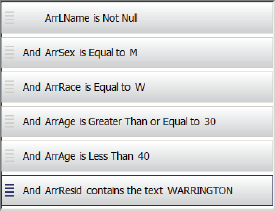
- 8.Click the SQL button to see the command that you just built. A new SQL logical operator is LIKE, which is used only on text-valued attributes. The value, WARRINGTON, is enclosed in single quote marks so that SQL learns that it’s a text value, and the % symbol is the wildcard character for ArcGIS SQL that stands for zero, one, or more characters to ignore. The record that you’ll retrieve has the value 1005 E WARRINGTON AV for ArrResid. The first % in the query value (‘%WARRINGTON%’) ignores seven characters at the beginning of the address (1005 E ), where the blank spaces are counted as characters, and the last % ignores three characters at the end ( AV).

- 9.Run the command. You now have an arrested person who may also have committed the unsolved burglary, John Bond.
- 10.Clear the selection, close the table, close the Geoprocessing pane, and save your project.
Tutorial 4-5: Data aggregation with a spatial join
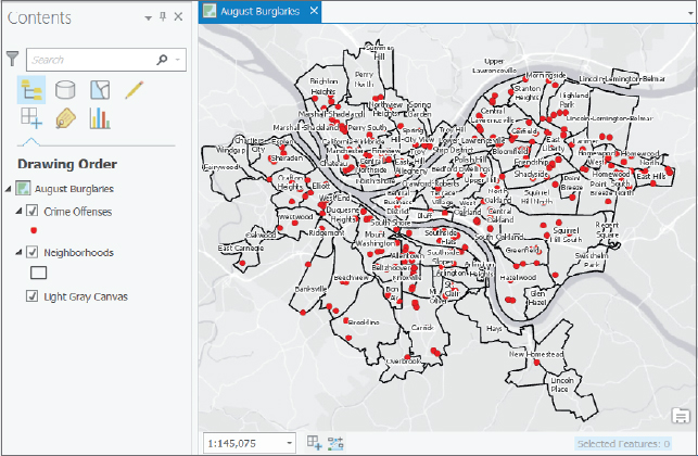
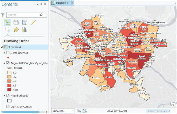
In this tutorial, you will count (aggregate) burglaries by neighborhood, providing the “big picture” of crime. Aggregation of point data requires a spatial join of burglary points to neighborhood polygons. The spatial join’s algorithm can sense the polygon in which a point lies, enabling the data aggregation. You’ll use the results to create a choropleth map of burglaries by neighborhood in August 2015. All of this is easy in ArcGIS Pro.
Open the Tutorial 4-5 project
- 1.Open Tutorial4-5.aprx in Chapter4\Tutorials, and save it as Tutorial4-5YourName.aprx.
- 2.Use the Pittsburgh bookmark. The map is the one that you used in tutorial 4-4 with the definition query yielding burglaries in August 2015. Neighborhood labels have been added and streets removed.
Build a spatial join
- 1.Search for and open the Spatial Join tool.
- 2.Type or make the selections as shown next. In the Output Fields list, starting with Area, point to each field and click the red x remove button so that only Name (from Neighborhoods) remains. When skipping over Name to remove Shape_Length, make sure that Name is not also selected before clicking the red x. Notice that Neighborhoods, the polygon outputs you need, are Target Features. Make sure that Keep All Target Features is selected so that polygons are output for neighborhoods that had no burglaries.

- 3.Click Run.
- 4.Close the Geoprocessing pane, and open the new map layer’s attribute table. See that Join_Count is added as a new attribute and is equal to the number of burglaries in each neighborhood.
- 5.Close the table.
YOUR TURN
Create a choropleth map using Join_Count from August2015BurglariesByNeighborhood. Use five quantiles and the color scheme of your choice. When finished, save and close your project.
Tutorial 4-6: Central point features for polygons
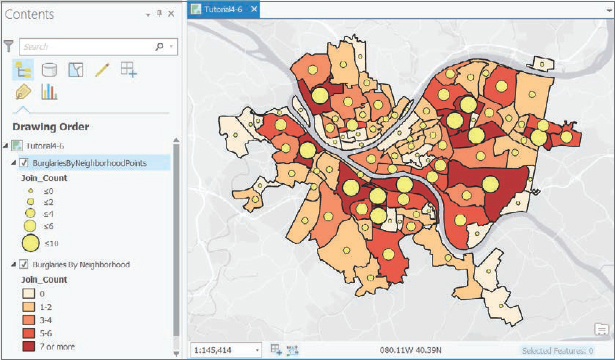
If you choose graduated symbols for symbology of a polygon map layer, ArcGIS Pro creates the central points on the fly and renders them as point features. This choice works well and saves you the work of creating a new central point feature class from the polygons yourself. However, it is often helpful to create a separate feature class with central points created from polygon features, so you will create a separate feature class.
Get started
- 1.Open Tutorial4-5.aprx from Chapter4\Tutorials, and save it as Tutorial4-6YourName.aprx.
- 2.Use the Pittsburgh bookmark. This map has the aggregate number of burglaries by neighborhood in Pittsburgh that you created in tutorial 4-5, without the neighborhood labels.
Create a central point feature class for polygons
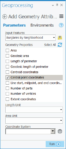
The centroid of a polygon is the arithmetic mean of all points within the polygon. For most polygons, centroids lie within their polygons, but for some, such as a quarter-moon-shaped polygon, centroids lie outside. If you want all center points to lie within their polygons, the remedy in ArcGIS is to use “central points” instead of centroids. Central points all lie within their polygons. In this tutorial, you’ll use the Feature To Point tool to create a central point feature class. Although not necessary, for practice you’ll first use the Add Geometry Attributes tool for adding central point coordinate attributes to the feature class. It’s valuable to know about the Add Geometry Attributes tool.
- 1.Search for and open the Add Geometry Attributes tool.
- 2.Make the selections as shown.
- 3.Run the tool.
- 4.Close the Geoprocessing pane and open the Burglaries By Neighborhood attribute table. The tool created Inside_X and Inside_Y central point coordinates, in State Plane feet.
- 5.Close the attribute table.
Create a new point layer
The Feature To Point tool creates a point layer of central points for polygons.
- 1.Search for and open the Feature To Point tool.
- 2.Select Burglaries By Neighborhood as Input Features, type BurglariesByNeighborhoodPoints for Output Feature Class, select Inside, and run the tool.
- 3.Run the tool, and when it finishes, close the tool.
YOUR TURN
Symbolize BurglariesByNeighborhoodPoints with graduated symbols using Join_Count with five quantiles. Although not required here, you could have changed the name of the Join_Count field to Burglaries to make the feature layer more self-documenting. You now have a point layer that could be used with a choropleth map of some other attribute by neighborhood, such as population living in poverty, and you could publish both in ArcGIS Online.
Tutorial 4-7: Create a new table for a one-to-many join
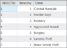
Data in a database commonly has a code field that, by itself, is not self-documenting. For example, crime data may have as crime type only the FBI hierarchy code, 1 through 7. The meaning of these codes is 1 = Criminal Homicide, 2 = Forcible Rape, 3 = Robbery, 4 = Aggravated Assault, 5 = Burglary, 6 = Larceny-Theft, and 7 = Motor Vehicle Theft. To break the code, you need a code table with the seven codes in one field and the descriptions in a second field. In this tutorial, you’ll create the code table, create a template for its fields, enter data into it, and join the table to crime data. This join is called “one to many,” because the same code table record—for example, the one for homicide—is joined to many crime incidents, all of them homicides.
You can use a field domain (see chapter 12) as an alternative approach for adding code values such as crime type to a table. This alternative is most relevant when the descriptive name of the code is itself the code (and there are no cryptic code values such as the FBI hierarchy). The code values become part of the table so that, for example, when responding police officers enter new crime data using Collector for ArcGIS, Collector’s data entry form automatically has a drop list with all crime types available for selection, rather than requiring a user to type. A drop list improves data integrity because crime type codes are not typed but selected from the drop list. This feature eliminates the potential of misspelled words and guarantees that the user will retrieve all relevant records—for example, after a query of all crimes of a certain type.
Open the Tutorial 4-7 project
- 1.Open Tutorial4-7.aprx from Chapter4\Tutorials, and save it as Tutorial4-7YourName.aprx.
- 2.Use the Pittsburgh bookmark.
Create a new table
- 1.Search for and open the Create Table tool.
- 2.For table name, type UCRHierarchyCode.
- 3.Run the tool, and when it finishes, close the Geoprocessing pane.
YOUR TURN
Open the Fields design view of UCRHierarchyCode, and add two new fields: Hierarchy with the short data type and Crime with the text data type and length 25. Then open the table, and type seven records as shown next. Note that ArcGIS Pro automatically enters values for ObjectID, so you don’t have to type them. Click Edit and then Save when finished.
Make a one-to-many join
You’ll join your new code table to the map’s crime layer to make crime type available for use.
- 1.Look at the attribute table for PittsburghSeriousCrimesSummer2015, and see that it has Hierarchy as a field, but not crime type.
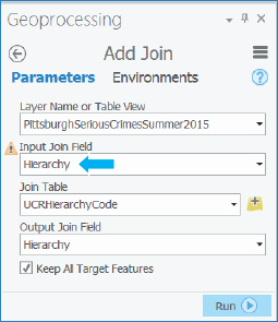
- 2.Right-click PittsburghSeriousCrimesSummer2015, click Joins and Relates > Add Join, and make the selections as shown.
- 3.Run the tool, and when it finishes, close it.
- 4.Look at the crime attribute table again, and see the joined attributes.
YOUR TURN
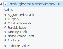
Symbolize PittsburghSeriousCrimesSummer2015 with unique values and Crime as the value field. Although you could improve symbolization of crimes by giving each crime a different shaped symbol, you’ll not do that work here. The point is that you can see that the code table has benefited, with the legend in the Contents pane labeled with crime types. When you finish, save and close your project.
Assignments
This chapter has three assignments to complete that you can download from this book’s resource web page, esri.com/gist1arcgispro:
- Assignment 4-1: Investigate the spatial distribution of PhDs in Allegheny County.
- Assignment 4-2: Compare serious violent crime with poverty in Pittsburgh.
- Assignment 4-3: Query statistics for day and night burglaries and larcenies by month.