Whatever your occupation, you often have to assess whether something new and different has happened. Sometimes you start with a population that you know a lot about (like its mean and standard deviation) and you draw a sample. Is that sample like the rest of the population, or does it represent something out of the ordinary?
To answer that question, you measure each individual in the sample and calculate the sample’s statistics. Then you compare those statistics with the population’s parameters. Are they the same? Are they different? Is the sample extraordinary in some way? Proper use of statistics helps you make the decision.
Sometimes, though, you don’t know the parameters of the population that the sample came from. What happens then? In this chapter, I discuss statistical techniques and R functions for dealing with both cases.
Hypotheses, Tests, and Errors
A hypothesis is a guess about the way the world works. It's a tentative explanation of some process, whether that process occurs in nature or in a laboratory.
Before studying and measuring the individuals in a sample, a researcher formulates hypotheses that predict what the data should look like.
Generally, one hypothesis predicts that the data won't show anything new or out of the ordinary. This is called the null hypothesis (abbreviated H0). According to the null hypothesis, if the data deviates from the norm in any way, that deviation is due strictly to chance. Another hypothesis, the alternative hypothesis (abbreviated H1), explains things differently. According to the alternative hypothesis, the data show something important.
After gathering the data, it’s up to the researcher to make a decision. The way the logic works, the decision centers around the null hypothesis. The researcher must decide to either reject the null hypothesis or to not reject the null hypothesis.
In hypothesis testing, you
Formulate null and alternative hypotheses
Gather data
Decide whether to reject or not reject the null hypothesis.
Nothing in the logic involves accepting either hypothesis. Nor does the logic involve making any decisions about the alternative hypothesis. It's all about rejecting or not rejecting H0.
Regardless of the reject-don’t-reject decision, an error is possible. One type of error occurs when you believe that the data shows something important and you reject H0, but in reality the data are due just to chance. This is called a Type I error. At the outset of a study, you set the criteria for rejecting H0. In so doing, you set the probability of a Type I error. This probability is called alpha (α).
The other type of error occurs when you don’t reject H0 and the data is really due to something out of the ordinary. For one reason or another, you happened to miss it. This is called a Type II error. Its probability is called beta (β). Table 10-1 summarizes the possible decisions and errors.
TABLE 10-1 Decisions and Errors in Hypothesis Testing
“True State” of the World
H0 is True
H1 is True
Reject H0
Type I Error
Correct Decision
Decision
Do Not Reject H0
Correct Decision
Type II Error
Note that you never know the true state of the world. (If you do, it’s not necessary to do the study!) All you can ever do is measure the individuals in a sample, calculate the statistics, and make a decision about H0. (I discuss hypotheses and hypothesis testing in Chapter 1.)
Hypothesis Tests and Sampling Distributions
In Chapter 9, I discuss sampling distributions. A sampling distribution, remember, is the set of all possible values of a statistic for a given sample size.
Also in Chapter 9, I discuss the central limit theorem. This theorem tells you that the sampling distribution of the mean approximates a normal distribution if the sample size is large (for practical purposes, at least 30). This works whether or not the population is normally distributed. If the population is a normal distribution, the sampling distribution is normal for any sample size. Here are two other points from the central limit theorem:
The mean of the sampling distribution of the mean is equal to the population mean.
The equation for this is
The standard error of the mean (the standard deviation of the sampling distribution) is equal to the population standard deviation divided by the square root of the sample size.
This equation is
The sampling distribution of the mean figures prominently into the type of hypothesis testing I discuss in this chapter. Theoretically, when you test a null hypothesis versus an alternative hypothesis, each hypothesis corresponds to a separate sampling distribution.
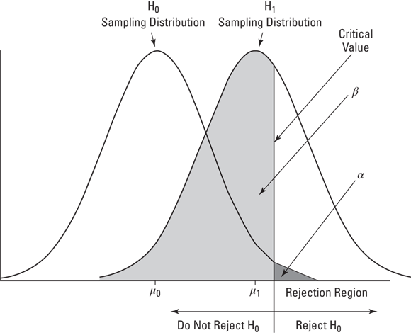
Figure 10-1 shows what I mean. The figure shows two normal distributions. I placed them arbitrarily. Each normal distribution represents a sampling distribution of the mean. The one on the left represents the distribution of possible sample means if the null hypothesis is truly how the world works. The one on the right represents the distribution of possible sample means if the alternative hypothesis is truly how the world works.
FIGURE 10-1: H0 and H1 each correspond to a sampling distribution.
Of course, when you do a hypothesis test, you never know which distribution produces the results. You work with a sample mean — a point on the horizontal axis. The reject-or-don’t reject decision boils down to deciding which distribution the sample mean is part of. You set up a critical value — a decision criterion. If the sample mean is on one side of the critical value, you reject H0. If not, you don't.
In this vein, the figure also shows α and β. These, as I mention earlier in this chapter, are the probabilities of decision errors. The area that corresponds to α is in the H0 distribution. I’ve shaded it in dark gray. It represents the probability that a sample mean comes from the H0 distribution, but it’s so extreme that you reject H0.
Where you set the critical value determines α. In most hypotheses testing, you set α at .05. This means that you're willing to tolerate a Type I error (rejecting H0 when you shouldn’t) 5 percent of the time. Graphically, the critical value cuts off 5 percent of the area of the sampling distribution. By the way, if you're talking about the 5 percent of the area that's in the right tail of the distribution (refer to Figure 10-1), you're talking about the upper 5 percent. If it’s the 5 percent in the left tail you're interested in, that's the lower 5 percent.
The area that corresponds to β is in the H1 distribution. I’ve shaded it in light gray. This area represents the probability that a sample mean comes from the H1 distribution, but it's close enough to the center of the H0 distribution that you don't reject H0 (but you should have). You don't get to set β. The size of this area depends on the separation between the means of the two distributions, and that’s up to the world we live in — not up to you.
These sampling distributions are appropriate when your work corresponds to the conditions of the central limit theorem: if you know that the population you're working with is a normal distribution or if you have a large sample.
Catching Some Z’s Again
Here's an example of a hypothesis test that involves a sample from a normally distributed population. Because the population is normally distributed, any sample size results in a normally distributed sampling distribution. Because it's a normal distribution, you use z-scores in the hypothesis test:
One more “because”: Because you use the z-score in the hypothesis test, the z-score here is called the test statistic.
Suppose you think that people living in a particular zip code have higher-than-average IQs. You take a sample of nine people from that zip code, give them IQ tests, tabulate the results, and calculate the statistics. For the population of IQ scores, μ = 100 and σ = 15.
The hypotheses are
H0: μZIP code ≤ 100
H1: μZIP code > 100
Assume that α = .05. That's the shaded area in the tail of the H0 distribution in Figure 10-1.
Why the ≤ in H0? You use that symbol because you'll reject H0 only if the sample mean is larger than the hypothesized value. Anything else is evidence in favor of not rejecting H0.
Suppose the sample mean is 108.67. Can you reject H0?
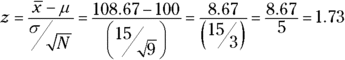
The test involves turning 108.67 into a standard score in the sampling distribution of the mean:
Is the value of the test statistic large enough to enable you to reject H0 with α = .05? It is. The critical value — the value of z that cuts off 5 percent of the area in a standard normal distribution — is 1.645. (After years of working with the standard normal distribution, I happen to know this. Read Chapter 8, find out about R’s qnorm() function, and you can have information like that at your fingertips, too.) The calculated value, 1.73, exceeds 1.645, so it's in the rejection region. The decision is to reject H0.
This means that if H0 is true, the probability of getting a test statistic value that's at least this large is less than .05. That's strong evidence in favor of rejecting H0.
In statistical parlance, any time you reject H0, the result is said to be statistically significant.
This type of hypothesis testing is called one-tailed because the rejection region is in one tail of the sampling distribution.
A hypothesis test can be one-tailed in the other direction. Suppose you have reason to believe that people in that zip code have lower-than-average IQs. In that case, the hypotheses are
H0: μZIP code ≥ 100
H1: μZIP code < 100
For this hypothesis test, the critical value of the test statistic is –1.645 if α = .05.
A hypothesis test can be two-tailed, meaning that the rejection region is in both tails of the H0 sampling distribution. That happens when the hypotheses look like this:
H0: μZIP code = 100
H1: μZIP code ≠ 100
In this case, the alternative hypothesis just specifies that the mean is different from the null-hypothesis value, without saying whether it's greater or whether it's less. Figure 10-2 shows what the two-tailed rejection region looks like for α = .05. The 5 percent is divided evenly between the left tail (also called the lower tail) and the right tail (the upper tail).
FIGURE 10-2: The two-tailed rejection region for α = .05.
For a standard normal distribution, incidentally, the z-score that cuts off 2.5 percent in the right tail is 1.96. The z-score that cuts off 2.5 percent in the left tail is –1.96. (Again, I happen to know these values after years of working with the standard normal distribution.) The z-score in the preceding example, 1.73, does not exceed 1.96. The decision, in the two-tailed case, is to not reject H0.
This brings up an important point. A one-tailed hypothesis test can reject H0, while a two-tailed test on the same data might not. A two-tailed test indicates that you’re looking for a difference between the sample mean and the null-hypothesis mean, but you don’t know in which direction. A one-tailed test shows that you have a pretty good idea of how the difference should come out. For practical purposes, this means you should try to have enough knowledge to be able to specify a one-tailed test: That gives you a better chance of rejecting H0 when you should.
Z Testing in R
An R function called z.test() would be great for doing the kind of testing I discuss in the previous section. One problem: That function does not exist in base R. Although you can find one in other packages, it’s easy enough to create one and learn a bit about R programming in the process.
The function will work like this:
> IQ.data <- c(100,101,104,109,125,116,105,108,110) > z.test(IQ.data,100,15) z = 1.733 one-tailed probability = 0.042 two-tailed probability = 0.084
Begin by creating the function name and its arguments:
z.test = function(x,mu,popvar){
The first argument is the vector of data, the second is the population mean, and the third is the population variance. The left curly bracket signifies that the remainder of the code is what happens inside the function.
Next, create a vector that will hold the one-tailed probability of the z-score you’ll calculate:
one.tail.p <- NULL
Then you calculate the z-score and round it to three decimal places:
Why put abs() (absolute value) in the argument to pnorm? Remember that an alternative hypothesis can specify a value below the mean, and the data might result in a negative z-score.
The next order of business is to set up the output display. For this, you use the cat() function. I use this function in Chapter 7 to display a fairly sizable set of numbers in an organized way. The name cat is short for concatenate and print, which is exactly what I want you to do here: Concatenate (put together) strings (like one-tailed probability =) with expressions (like one.tail.p), and then show that whole thing onscreen. I also want you to start a new line for each concatenation, and \n is R’s way of making that happen.
Here’s the cat statement:
cat(" z =",z.score,"\n", "one-tailed probability =", one.tail.p,"\n", "two-tailed probability =", 2*one.tail.p )}
The space between the left quote and z lines up the first line with the next two onscreen. The right curly bracket closes off the function.
Here it is, all together:
z.test = function(x,mu,popvar){ one.tail.p <- NULL z.score <- round((mean(x)-mu)/(popvar/sqrt(length(x))),3) one.tail.p <- round(pnorm(abs(z.score),lower.tail = FALSE),3) cat(" z =",z.score,"\n", "one-tailed probability =", one.tail.p,"\n", "two-tailed probability =", 2*one.tail.p )}
Running this function produces what you see at the beginning of this section.
t for One
In the preceding example, you work with IQ scores. The population of IQ scores is a normal distribution with a well-known mean and standard deviation. Thus, you can work with the central limit theorem and describe the sampling distribution of the mean as a normal distribution. You can then use z as the test statistic.
In the real world, however, you usually don’t have the luxury of working with well-defined populations. You usually have small samples, and you're typically measuring something that isn't as well-known as IQ. The bottom line is that you often don't know the population parameters, nor do you know if the population is normally distributed.
When that’s the case, you use the sample data to estimate the population standard deviation, and you treat the sampling distribution of the mean as a member of a family of distributions called the t-distribution. You use t as a test statistic. In Chapter 9, I introduce this distribution and mention that you distinguish members of this family by a parameter called degrees of freedom (df).
The formula for the test statistic is
Think of df as the denominator of the estimate of the population variance. For the hypothesis tests in this section, that's N–1, where N is the number of scores in the sample. The higher the df, the more closely the t-distribution resembles the normal distribution.
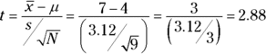
Here's an example. FarKlempt Robotics, Inc., markets microrobots. The company claims that its product averages four defects per unit. A consumer group believes this average is higher. The consumer group takes a sample of nine FarKlempt microrobots and finds an average of seven defects, with a standard deviation of 3.12. The hypothesis test is
H0: μ ≤ 4
H1: μ > 4
α = .05
The formula is
Can you reject H0? The R function in the next section tells you.
t Testing in R
I preview the t.test() function in Chapter 2 and talk about it in a bit more detail in Chapter 9. Here, you use it to test hypotheses.
Start with the data for FarKlempt Robotics:
> FarKlempt.data <- c(3,6,9,9,4,10,6,4,12)
Then apply t.test(). For the example, it looks like this:
The second argument specifies that you’re testing against a hypothesized mean of 4, and the third argument indicates that the alternative hypothesis is that the true mean is greater than 4.
Here it is in action:
> t.test(FarKlempt.data,mu=4, alternative="greater") One Sample t-test data: c(3, 6, 9, 9, 4, 10, 6, 4, 12) t = 2.8823, df = 8, p-value = 0.01022 alternative hypothesis: true mean is greater than 4 95 percent confidence interval: 5.064521 Inf sample estimates: mean of x 7
The output provides the t-value and the low p-value shows that you can reject the null hypothesis with α = .05.
This t.test() function is versatile. I work with it again in Chapter 11 when I test hypotheses about two samples.
Working with t-Distributions
Just as you can use d, p, q, and r prefixes for the normal distribution family, you can use dt() (density function), pt() (cumulative density function), qt() (quantiles), and rt() (random number generation) for the t-distribution family.
Here are dt() and rt() at work for a t-distribution with 12 df:
All these functions give you the option of working with t-distributions not centered around zero. You do this by entering a value for ncp (the noncentrality parameter). In most applications of the t-distribution, noncentrality doesn’t come up. For completeness, I explain this concept in greater detail in Appendix 3 online.
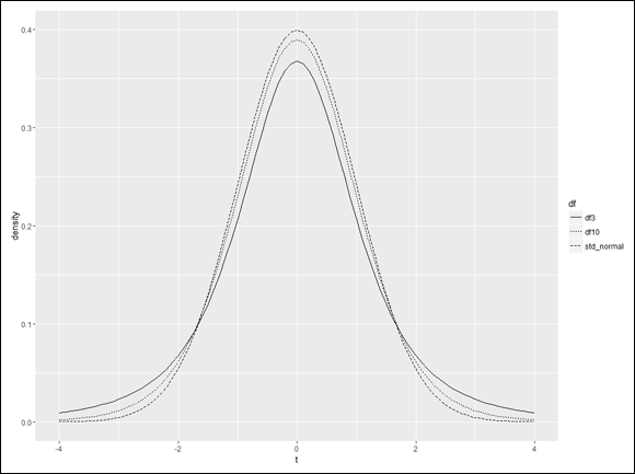
Visualizing t-Distributions
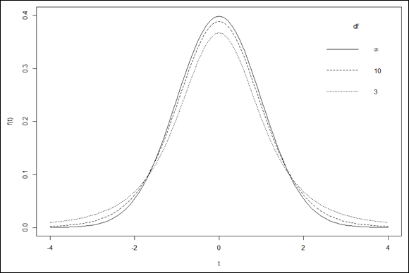
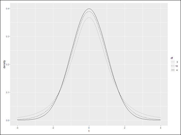
Visualizing a distribution often helps you understand it. The process can be a bit involved in R, but it’s worth the effort. Figure 9-7 shows three members of the t-distribution family on the same graph. The first has df=3, the second has df=10, and the third is the standard normal distribution (df=infinity).
In this section, I show you how to create that graph in base R graphics and in ggplot2.
With either method, the first step is to set up a vector of the values that the density functions will work with:
t.values <- seq(-4,4,.1)
One more thing and I’ll get you started. After the graphs are complete, you’ll put the infinity symbol, on the legends to denote the df for the standard normal distribution. To do that, you have to install a package called grDevices: On the Packages tab, click Install, and then in the Install Packages dialog box, type grDevices and click Install. When grDevices appears on the Packages tab, select its check box.
With grDevices installed, this adds the infinity symbol to a legend:
expression(infinity)
But I digress… .
Plotting t in base R graphics
Begin with the plot() function, and plot the t-distribution with 3 df:
The first two arguments are pretty self-explanatory. The next two establish the type of plot — type = “l” means line plot (that’s a lowercase “L” not the number 1), and lty = “dotted” indicates the type of line. The ylim argument sets the lower and upper limits of the y-axis — ylim = c(0,.4). A little tinkering shows that if you don’t do this, subsequent curves get chopped off at the top. The final two arguments label the axes. Figure 10-3 shows the graph so far:
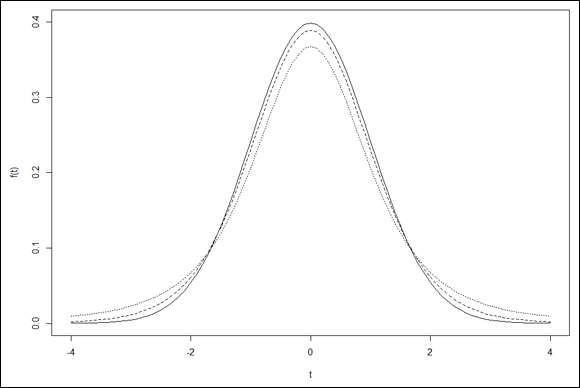
The line for the standard normal is solid (the default value for lty). Figure 10-4 shows the progress. All that’s missing is the legend that explains which curve is which.
FIGURE 10-4: Three distributions in search of a legend.
One advantage of base R is that positioning and populating the legend is not difficult:
The first argument positions the legend in the upper-right corner. The second gives the legend its title. The third argument is a vector that specifies what’s in the legend. As you can see, the first element is that infinity expression I showed you earlier, corresponding to the df for the standard normal. The second and third elements are the df for the remaining two t-distributions. You order them this way because that’s the order in which the curves appear at their centers. The lty argument is the vector that specifies the order of the linetypes (they correspond with the df). The final argument bty="n" removes the border from the legend.
That’s a pretty good-looking data frame, but it’s in wide format. As I point out in Chapter 3, ggplot() prefers long format — which is the three columns of density-numbers stacked into a single column. To get to that format — it’s called reshaping the data — make sure you have the reshape2 package installed. Select its check box on the Packages tab and you’re ready to go.
Reshaping from wide format to long format is called melting the data, so the function is
t.frame.melt <- melt(t.frame,id="t.values")
The id argument specifies that t.values is the variable whose numbers don’t get stacked with the rest. Think of it as the variable that stores the data. The first six rows of t.frame.melt are:
Now for one more thing before I have you start on the graph. This is a vector that will be useful when you lay out the x-axis:
x.axis.values <- seq(-4,4,2)
Begin with ggplot():
ggplot(t.frame.melt, aes(x=t,y=f(t),group =df))
The first argument is the data frame. The aesthetic mappings tell you that t is on the x-axis, density is on the y-axis, and the data falls into groups specified by the df variable.
This is a line plot, so the appropriate geom function to add is geom_line:
geom_line(aes(linetype=df))
Geom functions can work with aesthetic mappings. The aesthetic mapping here maps df to the type of line.
Rescale the x-axis so that it goes from –4 to 4, by twos. Here’s where to use that x.axis.values vector:
FIGURE 10-7: Three t-distribution curves, with the linetypes reassigned.
As you can see, the items in the legend are not in the order that the curves appear at their centers. I’m a stickler for that. I think it makes a graph more comprehensible when the graph elements and the legend elements are in sync. ggplot2 provides guide functions that enable you to control the legend’s details. To reverse the order of the linetypes in the legend, here’s what you do:
guides(linetype=guide_legend(reverse = TRUE))
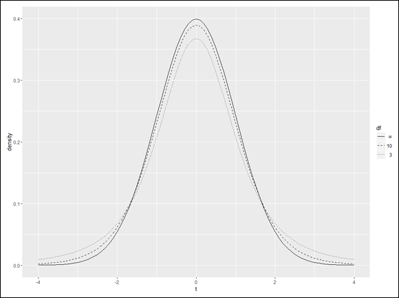
Putting all the code together, finally, yields Figure 10-8.
FIGURE 10-8: The final product, with the legend rearranged.
I leave it to you as an exercise to relabel the y-axis f(t).
Base R graphics versus ggplot2: It’s like driving a car with a standard transmission versus driving with an automatic transmission — but I’m not always sure which is which!
One more thing about ggplot2
I could have had you plot all this without creating and reshaping a data frame. An alternative approach is to set NULL as the data source, map t.values to the x-axis, and then add three geom_line statements. Each of those statements would map a vector of densities (created on the fly) to the y-axis, and each one would have its own linetype.
The problem with that approach? When you do it that way, the grammar does not automatically create a legend. Without a data frame, it has nothing to create a legend from. It’s something like using ggplot() to create a base R graph.
Is it ever a good idea to use this approach? Yes, it is — when you don’t want to include a legend but you want to annotate the graph in some other way. I provide an example in the later section “Visualizing Chi-Square Distributions.”
Testing a Variance
So far, I discuss one-sample hypothesis testing for means. You can also test hypotheses about variances.
This topic sometimes comes up in the context of manufacturing. Suppose FarKlempt Robotics, Inc., produces a part that has to be a certain length with a very small variability. You can take a sample of parts, measure them, find the sample variability, and perform a hypothesis test against the desired variability.
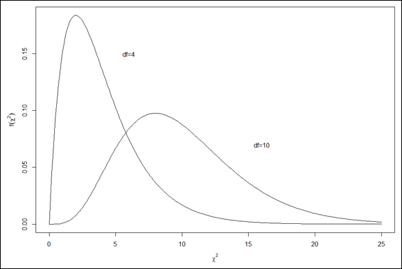
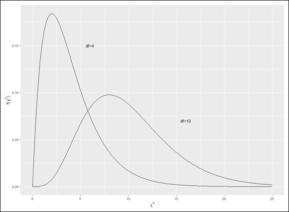
The family of distributions for the test is called chi-square. Its symbol is χ2. I won't go into all the mathematics. I'll just tell you that, once again, df is the parameter that distinguishes one member of the family from another. Figure 10-9 shows two members of the chi-square family.
FIGURE 10-9: Two members of the chi-square family.
As the figure shows, chi-square is not like the previous distribution families I showed you. Members of this family can be skewed, and none of them can take a value less than zero.
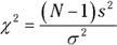
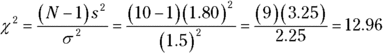
The formula for the test statistic is
N is the number of scores in the sample, s2 is the sample variance, and σ2 is the population variance specified in H0.
With this test, you have to assume that what you’re measuring has a normal distribution.
Suppose the process for the FarKlempt part has to have, at most, a standard deviation of 1.5 inches for its length. (Notice that I use standard deviation. This allows me to speak in terms of inches. If I use variance, the units would be square inches.) After measuring a sample of 10 parts, you find a standard deviation of 1.80 inches.
The hypotheses are
H0: σ2 ≤ 2.25 (remember to square the “at-most” standard deviation of 1.5 inches)
H1: σ2 > 2.25
α = .05
Working with the formula,
can you reject H0? Read on.
Testing in R
At this point, you might think that the function chisq.test() would answer the question. Although base R provides this function, it’s not appropriate here. As you can see in Chapters 18 and 20, statisticians use this function to test other kinds of hypotheses.
Instead, turn to a function called varTest, which is in the EnvStats package. On the Packages tab, click Install. Then type EnvStats into the Install Packages dialog box and click Install. When EnvStats appears on the Packages tab, select its check box.
Before you use the test, you create a vector to hold the ten measurements described in the example in the preceding section:
The first argument is the data vector. The second specifies the alternative hypothesis that the true variance is greater than the hypothesized variance, the third gives the confidence level (1–α), and the fourth is the hypothesized variance.
Running that line of code produces these results:
Results of Hypothesis Test -------------------------- Null Hypothesis: variance = 2.25 Alternative Hypothesis: True variance is greater than 2.25 Test Name: Chi-Squared Test on Variance Estimated Parameter(s): variance = 3.245299 Data: FarKlempt.data2 Test Statistic: Chi-Squared = 12.9812 Test Statistic Parameter: df = 9 P-value: 0.163459 95% Confidence Interval: LCL = 1.726327 UCL = Inf
Among other statistics, the output shows the chi-square (12.9812) and the p-value (0.163459). (The chi-square value in the previous section is a bit lower because of rounding.) The p-value is greater than .05. Therefore, you cannot reject the null hypothesis.
How high would chi-square (with df=9) have to be in order to reject? Hmmm… .
Working with Chi-Square Distributions
As is the case for the distribution families I’ve discussed in this chapter, R provides functions for working with the chi-square distribution family: dchisq() (for the density function), pchisq() (for the cumulative density function), qchisq() (for quantiles), and rchisq() (for random-number generation).
To answer the question I pose at the end of the previous section, I use qchisq():
Figure 10-9 nicely shows a couple of members of the chi-square family, with each member annotated with its degrees of freedom. In this section, I show you how to use base R graphics and ggplot2 to re-create that picture. You’ll learn some more about graphics, and you’ll know how to visualize any member of this family.
Plotting chi-square in base R graphics
To get started, you create a vector of values from which dchisq() calculates densities:
chi.values <- seq(0,25,.1)
Start the graphing with a plot statement:
plot(x=chi.values, y=dchisq(chi.values,df=4), type = "l", xlab=expression(chi^2), ylab="")
The first two arguments indicate what you’re plotting — the chi-square distribution with four degrees of freedom versus the chi.values vector. The third argument specifies a line (that’s a lowercase “L”, not the number 1). The third argument labels the x-axis with the Greek letter chi (χ) raised to the second power. The fourth argument gives the y-axis a blank label.
Why did I have you do that? When I first created the graph, I found that ylab locates the y-axis label too far to the left, and the label was cut off slightly. To fix that, I blank out ylab and then use mtext():
mtext(side = 2, text = expression(f(chi^2)), line = 2.5)
The side argument specifies the side of the graph to insert the label: bottom = 1, left = 2, top = 3, and right = 4. The text argument sets as the label for the axis. The line argument specifies the distance from the label to the y-axis: The distance increases with the value.
Next, you add the curve for chi-square with ten degrees of freedom:
lines(x=chi.values,y=dchisq(chi.values,df= 10))
Rather than add a legend, follow Figure 10-9 and add an annotation for each curve. Here’s how:
FIGURE 10-10: Two members of the chi-square family, plotted in base R graphics.
Plotting chi-square in ggplot2
In this plot, I again have you use annotations rather than a legend, so you set NULL as the data source and work with a vector for each line. The first aesthetic maps chi.values to the x-axis:
ggplot(NULL, aes(x=chi.values))
Then you add a geom_line for each chi-square curve, with the mapping to the y-axis as indicated:
As I point out earlier in this chapter, this is like using ggplot2 to create a base R graph, but in this case it works (because it doesn’t create an unwanted legend).
Next, you label the axes:
labs(x=expression(chi^2),y=expression(f(chi^2)))
And finally, the aptly named annotate() function adds the annotations:
 Introducing hypothesis tests
 Before studying and measuring the individuals in a sample, a researcher formulates hypotheses that predict what the data should look like.


 This brings up an important point. A one-tailed hypothesis test can reject H0, while a two-tailed test on the same data might not. A two-tailed test indicates that you’re looking for a difference between the sample mean and the null-hypothesis mean, but you don’t know in which direction. A one-tailed test shows that you have a pretty good idea of how the difference should come out. For practical purposes, this means you should try to have enough knowledge to be able to specify a one-tailed test: That gives you a better chance of rejecting H0 when you should.
 on the legends to denote the df for the standard normal distribution. To do that, you have to install a package called
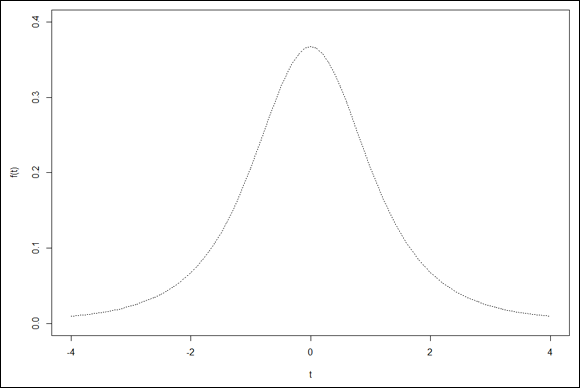

 as the label for the axis. The