Comparison Theory

The purpose of this chapter is to show how upper or lower bounds on curvature can be used to derive bounds on other geometric quantities such as lengths of tangent vectors, distances, and volumes. The intuition behind all the comparison theorems is that negative curvature forces geodesics to spread apart faster as you move away from a point, and positive curvature forces them to spread slower and eventually to begin converging.

One of the most useful comparison theorems is the Jacobi field comparison theorem (see Thm. 11.9 below), which gives bounds on the sizes of Jacobi fields based on curvature bounds. Its importance is based on four observations: first, in a normal neighborhood of a point p, every tangent vector can be represented as the value of a Jacobi field that vanishes at p (by Cor. 10.11); second, zeros of Jacobi fields correspond to conjugate points, beyond which geodesics cannot be minimizing; third, Jacobi fields represent the first-order behavior of families of geodesics; and fourth, each Jacobi field satisfies a differential equation that directly involves the curvature.

In the first section of the chapter, we set the stage for the comparison theorems by showing how the growth of Jacobi fields in a normal neighborhood is controlled by the Hessian of the radial distance function, which satisfies a first-order differential equation called a Riccati equation. We then state and prove a fundamental comparison theorem for Riccati equations.

Next we proceed to derive some of the most important geometric comparison theorems that follow from the Riccati comparison theorem. The first few comparison theorems are all based on upper or lower bounds on sectional curvatures. Then we explain how some comparison theorems can also be proved based on lower bounds for the Ricci curvature. In the next chapter, we will see how these comparison theorems can be used to prove significant local-to-global theorems in Riemannian geometry.

Since all of the results in this chapter are deeply intertwined with lengths and distances, we restrict attention throughout the chapter to the Riemannian case.

Jacobi Fields, Hessians, and Riccati Equations

Our main aim in this chapter is to use curvature inequalities to derive consequences about how fast the metric grows or shrinks, based primarily on size estimates for Jacobi fields. But first, we need to make one last stop along the way.

The Jacobi equation is a second-order differential equation, but comparison theory for differential equations generally works much more smoothly for first-order equations. In order to get the sharpest results about Jacobi fields and other geometric quantities, we will derive a first-order equation, called a Riccati equation, that is closely related to the Jacobi equation.

Let (M, g) be an n-dimensional Riemannian manifold, let U be a normal neighborhood of a point $p\in M$ , and let $r:U\mathrel {\rightarrow }\mathbb {R}$ be the radial distance function as defined by (6.4). The Gauss lemma shows that the gradient of r on $U\smallsetminus \{p\}$ is the radial vector field $\partial _r$ .

On $U\smallsetminus \{p\}$ , we can form the symmetric covariant 2-tensor field $\nabla ^2 r$ (the covariant Hessian of r) and the (1, 1)-tensor field $\mathscr {H}_r = \nabla (\partial _r)$ . Because $\partial _r = {{\,\mathrm{grad}\,}}r = (\nabla r)^\sharp$ and $\nabla$ commutes with the musical isomorphisms (Prop. 5.17), we have

$\begin{aligned} \mathscr {H}_r = \nabla (\partial _r) = \nabla \big ((\nabla r)^\sharp \big ) = \big (\nabla ^2 r\big )^\sharp . \end{aligned}$

In other words, $\mathscr {H}_r$ is obtained from $\nabla ^2 r$ by raising one of its indices.

Using Proposition B.1, we can also interpret the (1, 1)-tensor field $\mathscr {H}_r$ as an element of $\Gamma \big (\mathrm{{End}}\big (TM|_{U\smallsetminus \{p\}}\big )\big )$ (that is, a field of endomorphisms of TM over $U\smallsetminus \{p\}$ ), defined by

$\begin{aligned} \mathscr {H}_r (w) = \nabla _w \partial _r \end{aligned}$

(11.1)

for all $w\in TM|_{U\smallsetminus \{p\}}$ . The endomorphism field $\mathscr {H}_r$ is called the Hessian operator of r. It is related to the (0, 2)-Hessian by

$\begin{aligned} \langle \mathscr {H}_r (v), w \rangle = \big (\nabla ^2 r\big )(v,w), \quad \text { for all } q\in U\smallsetminus \{p\}~\text {and}~v, w\in T_qM. \end{aligned}$

(11.2)

The next lemma summarizes some of its basic algebraic properties.

Lemma 11.1.

Let r, $\partial _r$ , and $\mathscr {H}_r$ be defined as above.

(a)
$\mathscr {H}_r$ is self-adjoint.
(b)
$\mathscr {H}_r(\partial _r)\equiv 0$ .
(c)
The restriction of $\mathscr {H}_r$ to vectors tangent to a level set of r is equal to the shape operator of the level set associated with the normal vector field $N = - \partial _r$ .

Proof.

Since the covariant Hessian $\nabla ^2 r$ is symmetric, equation (11.2) shows that the Hessian operator is self-adjoint. Part (b) follows immediately from the fact that $\mathscr {H}_r (\partial _r) = \nabla _{\partial _r} \partial _r = 0$ because the integral curves of $\partial _r$ are geodesics.

Next, note that $\partial _r$ is a unit vector field normal to each level set of r by the Gauss lemma, so (c) follows from the Weingarten equation 8.11. $\square$

Problem 11-1 gives another geometric interpretation of $\nabla ^2 r$ , as the radial derivative of the nonconstant components of the metric in polar normal coordinates.

The Hessian operator also has a close relationship with Jacobi fields.

Proposition 11.2.

Suppose (M, g) is a Riemannian manifold, $U\subseteq M$ is a normal neighborhood of $p\in M$ , and r is the radial distance function on U. If $\gamma :[0,b]\mathrel {\rightarrow }U$ is a unit-speed radial geodesic segment starting at p, and $J\in \mathscr {J}^\perp (\gamma )$ is a normal Jacobi field along $\gamma$ that vanishes at $$t=0$$

, then the following equation holds for all $t\in (0,b]$ :

$\begin{aligned} D_tJ(t) = \mathscr {H}_r(J(t)). \end{aligned}$

(11.3)

Proof.

Let $v = \gamma '(0)$ , so $$|v|_g = 1$$

and $\gamma (t) = \exp _p(tv)$ . Proposition 10.10 shows that

$\begin{aligned} J(t) = d\big (\exp _p\big )_{tv} (tw), \end{aligned}$

where $D_tJ(0) = w = w^i\partial _i|_{p}$ . Because we are assuming that J is normal, it follows from Proposition 10.7 that $w\perp v$ .

Because $w\perp v$ ensures that w is tangent to the unit sphere in $$T_pM$$

at v, we can choose a smooth curve $\sigma :(-\varepsilon ,\varepsilon )\mathrel {\rightarrow }T_pM$ that satisfies $|\sigma (s)|_g = 1$ for all $s\in (-\varepsilon ,\varepsilon )$ , with initial conditions $\sigma (0) = v$ and $\sigma '(0) = w$ . (As always, we are using the canonical identification between $$T_v(T_pM)$$

and

.) Define a smooth family of curves $\varGamma :(-\varepsilon ,\varepsilon )\times [0,b]\mathrel {\rightarrow }M$ by $\varGamma (s, t) = \exp _p( t \sigma (s))$ . Then $\varGamma (0,t)=\exp _p(tv) = \gamma (t)$ , so $\varGamma$ is a variation of $\gamma$ . The stipulation that $|\sigma (s)|_g \equiv 1$ ensures that each main curve $\varGamma _s(t) = \varGamma (s, t)$ is a unit-speed radial geodesic, so its velocity satisfies the following identity for all (s, t):

$\begin{aligned} \partial _t\varGamma (s,t) =(\varGamma _s)'(t) = \partial _r \big |_{\varGamma (s, t) }. \end{aligned}$

(11.4)

The chain rule yields

$\begin{aligned} \partial _s\varGamma (0,t) = d\big (\exp _p\big )_{t\sigma (0)} (t\sigma '(0)) = d\big (\exp _p\big )_{tv} (tw) = J(t), \end{aligned}$

so J is the variation field of $\varGamma$ . By the symmetry lemma,

$\begin{aligned} D_tJ(t) = D_t \partial _s \varGamma (0,t) = D_s \partial _t\varGamma (0,t). \end{aligned}$

(11.5)

This last expression is the covariant derivative of $\partial _t\varGamma (s, t)$ along the curve $\varGamma ^{(t)}(s) = \varGamma (s, t)$ evaluated at $$s=0$$

. Since the velocity of this curve at $$s=0$$

is $\partial _s\varGamma (0,t)=J(t)$ and $\partial _t\varGamma (s, t)=\partial _r$ is an extendible vector field by (11.4), we obtain

$\begin{aligned} D_s \partial _t\varGamma (0,t) = \nabla _{{\varGamma ^{(t)\prime }}(0)} (\partial _r) = \nabla _{J(t)}(\partial _r) = \mathscr {H}_r(J(t)). \end{aligned}$

Combining this with (11.5) yields the result. $\square$

In order to compare the Hessian operator of an arbitrary metric with those of the constant-curvature models, we need the following explicit formula for the constant-curvature case.

Proposition 11.3.

Suppose (M, g) is a Riemannian manifold, $U\subseteq M$ is a normal neighborhood of $p\in M$ , and r is the radial distance function on U. Then g has constant sectional curvature c on U if and only if the following formula holds at all points of $U\smallsetminus \{p\}$ :

$\begin{aligned} \mathscr {H}_r = \frac{s_c'(r)}{s_c(r)} \pi _r, \end{aligned}$

(11.6)

where

is defined by (10.8), and for each $q\in U\smallsetminus \{p\}$ , $\pi _r:T_qM\mathrel {\rightarrow }T_qM$ is the orthogonal projection onto the tangent space of the level set of r (equivalently, onto the orthogonal complement of $\partial _r|_q$ ).

Proof.

First suppose g has constant sectional curvature c on U. Let $q\in U\smallsetminus \{p\}$ , and let $\gamma :[0,b]\mathrel {\rightarrow }U$ be the unit-speed radial geodesic from p to q, so $$b=r(q)$$ . Let $(E_1,\dots , E_n)$ be a parallel orthonormal frame along $\gamma$ , chosen so that $E_n(t)= \gamma '(t) = \partial _r|_{\gamma (t)}$ . It follows from Proposition 10.12 that for $i=1,\dots , n-1$ , the vector fields $$J_i(t) = s_c(t) E_i(t)$$ are normal Jacobi fields along $\gamma$ that vanish at $$t=0$$ . The assumption that U is a normal neighborhood of p means that $U=\exp _p(V)$ for some star-shaped neighborhood V of $0\in T_pM$ , and every point of V is a regular point for $\exp _p$ . Thus Proposition 10.20 shows that p has no conjugate points along $\gamma$ , which implies that $s_c(t)\ne 0$ for $t\in (0,b]$ . (For $c\le 0$ , this is automatic, because $$s_c$$ vanishes only at 0; but in the case $$c=1/R^2 > 0$$ , it means that $b< \pi R$ .)

For $1\le i\le n-1$ , we use Proposition 11.2 to compute

$\begin{aligned} D_t J_i(t) = \mathscr {H}_r(J_i(t)) = s_c(t) \mathscr {H}_r(E_i(t)). \end{aligned}$

On the other hand, because each $$E_i$$

is parallel along $\gamma$ ,

$\begin{aligned} D_t J_i(t) = s_c'(t) E_i(t). \end{aligned}$

Comparing these two equations at $$t=b$$

and dividing by $$s_c(b)$$

, we obtain

$\begin{aligned} \mathscr {H}_r (E_i(b)) = \frac{s_c'(b)}{s_c(b)} E_i(b) = \frac{s_c'(b)}{s_c(b)} \pi _r(E_i(b)). \end{aligned}$

On the other hand, Lemma 11.1(b) shows that

$\begin{aligned} \mathscr {H}_r (E_n(b)) = \mathscr {H}_r\big (\partial _r|_q\big ) = 0 = \frac{s_c'(b)}{s_c(b)}\pi _r(E_n(b)), \end{aligned}$

because $\pi _r(E_n(b)) = \pi _r(\partial _r|_q) = 0$ . Since $$(E_i(b))$$

is a basis for $$T_qM$$

, this proves (11.6).

Conversely, suppose $\mathscr {H}_r$ is given by (11.6). Let $\gamma$ be a radial geodesic starting at p, and let J be a normal Jacobi field along $\gamma$ that vanishes at $$t=0$$ . By Proposition 11.2, $D_tJ(t) = \mathscr {H}_r J(t) = s_c'(t) J(t)/s_c(t)$ . A straightforward computation then shows that $s_c(t)^{-1}J(t)$ is parallel along $\gamma$ . Thus we can write every such Jacobi field in the form $$J(t) = k s_c(t) E(t)$$ for some constant k and some parallel unit normal vector field E along $\gamma$ . Proceeding exactly as in the proof of Theorem 10.14, we conclude that g is given by formula (10.17) in these coordinates, and therefore has constant sectional curvature c. $\square$

For convenience, we record the exact formulas for the quotient $$s_c'/s_c$$

that appeared in the previous proposition (see Fig. 11.1):

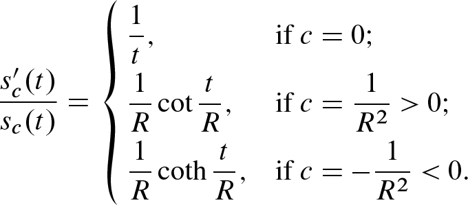
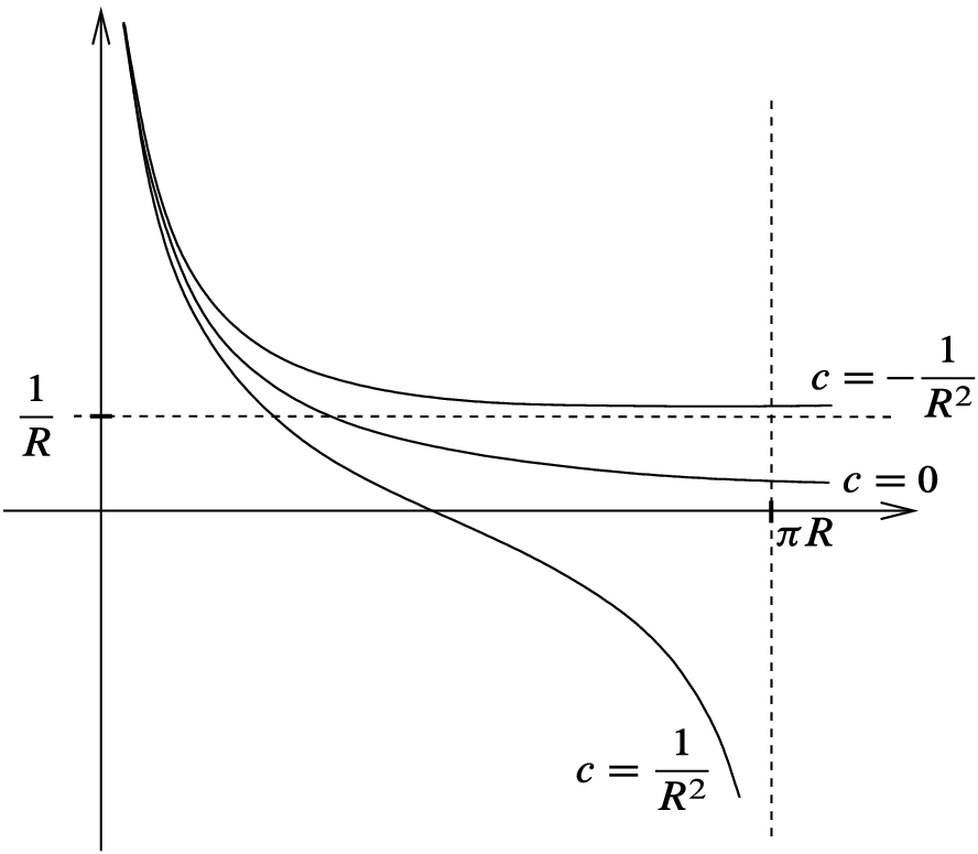
../images/56724_2_En_11_Chapter/56724_2_En_11_Equ84_HTML.png

../images/56724_2_En_11_Chapter/56724_2_En_11_Fig1_HTML.png — Fig. 11.1:
The graph of

Now we are in a position to derive the first-order equation mentioned at the beginning of this section. (Problem 11-3 asks you to show, with a different argument, that the conclusion of the next theorem holds for the Hessian operator of every smooth local distance function, not just the radial distance function in a normal neighborhood.) This theorem concerns the covariant derivative of the endomorphism field $\mathscr {H}_r$ along a curve $\gamma$ . We can compute the action of $D_t \mathscr {H}_r$ on every $V \in \mathfrak X(\gamma )$ by noting that $\mathscr {H}_r(V(t))$ is a contraction of $\mathscr {H}_r\otimes V(t)$ , so the product rule implies $D_t(\mathscr {H}_r (V)) = (D_t \mathscr {H}_r)V + \mathscr {H}_r(D_t V)$ .

Theorem 11.4

(The Riccati Equation). Let (M, g) be a Riemannian manifold; let U be a normal neighborhood of a point $p\in M$ ; let $r:U\mathrel {\rightarrow }\mathbb {R}$ be the radial distance function; and let $\gamma :[0,b]\mathrel {\rightarrow }U$ be a unit-speed radial geodesic. The Hessian operator $\mathscr {H}_r$ satisfies the following equation along $\gamma |_{(0,b]}$ , called a Riccati equation:

$\begin{aligned} D_t \mathscr {H}_r + \mathscr {H}_r^2 + R_{\gamma '} = 0, \end{aligned}$

(11.7)

where $\mathscr {H}_r^2$ and $R_{\gamma '}$ are the endomorphism fields along $\gamma$ defined by $\mathscr {H}_r^2(w) = \mathscr {H}_r(\mathscr {H}_r(w))$ and $R_{\gamma '}(w) = R\big (w,\gamma '\big )\gamma '$ , with R the curvature endomorphism of g.

Proof.

Let $t_0\in (0,b]$ and $w\in T_{\gamma (t_0)}M$ be arbitrary. We can decompose w as $$w = y+z$$ , where y is a multiple of $\partial _r$ and z is tangent to a level set of r. Since (11.7) is an equation between linear operators, we can prove the equation by evaluating it separately on y and z.

Because $\gamma$ is a unit-speed radial geodesic, its velocity is equal to $\partial _r$ , and thus $D_t\partial _r=0$ along $\gamma$ . It follows that $(D_t \mathscr {H}_r)(\partial _r) = D_t(\mathscr {H}_r(\partial _r)) - \mathscr {H}_r(D_t \partial _r) = 0$ . Since all three terms on the left-hand side of (11.7) annihilate $\partial _r$ , the equation holds when applied to any multiple of $\partial _r$ .

Next we consider a vector $z\in T_{\gamma (t_0)}M$ that is tangent to a level set of r, and thus by the Gauss lemma orthogonal to $\gamma '(t_0)$ . By Corollary 10.11, z can be expressed as the value at $$t=t_0$$

of a Jacobi field J along $\gamma$ vanishing at $$t=0$$

. Because J(0) and $$J(t_0)$$

are orthogonal to $\gamma '$ , it follows that J is a normal Jacobi field, so Proposition 11.2 shows that $D_tJ(t) = \mathscr {H}_r(J(t))$ for all $t\in [0,b]$ . Differentiation yields

$\begin{aligned} D_t^2 J = D_t(\mathscr {H}_r (J)) = (D_t \mathscr {H}_r)J + \mathscr {H}_r(D_t J) = (D_t \mathscr {H}_r)J + \mathscr {H}_r(\mathscr {H}_r(J)). \end{aligned}$

On the other hand, the Jacobi equation gives $D_t^2 J = - R_{\gamma '}(J)$ , so

$\begin{aligned} \big ( D_t \mathscr {H}_r + \mathscr {H}_r^2 + R_{\gamma '}\big )(J) \equiv 0. \end{aligned}$

Evaluating this at $$t=t_0$$

proves the result. $\square$

The Riccati equation is named after Jacopo Riccati, an eighteenth-century Italian mathematician who studied scalar differential equations of the form $$v' +pv^2 +qv +r=0$$ , where p, q, r are known functions and v is an unknown function of one real variable. As is shown in some ODE texts, a linear second-order equation in one variable of the form $$au'' + bu' + c u = 0$$ can be transformed to a Riccati equation wherever $u\ne 0$ by making the substitution $$v= u'/u$$ . The relation (11.3) generalizes this, and allows us to replace the analysis of the second-order linear Jacobi equation by an analysis of the first-order nonlinear Riccati equation.

The primary tool underlying all of our geometric comparison theorems is a fundamental comparison theorem for solutions to Riccati equations. It says, roughly, that a larger curvature term results in a smaller solution, and vice versa. When we apply this to (11.3), it will yield an analogous comparison for Jacobi fields.

In the statement and proof of this theorem, we will compare self-adjoint endomorphisms by comparing the quadratic forms they determine. Given a finite-dimensional inner product space V and self-adjoint endomorphisms $A, B:V\mathrel {\rightarrow }V$ , the notation $A\le B$ means that $\langle Av,v\rangle \le \langle Bv, v\rangle$ for all $v\in V$ , or equivalently that $$B-A$$ is positive semidefinite. In particular, $B\ge 0$ means that B is positive semidefinite. Note that the square of every self-adjoint endomorphism is positive semidefinite, because $\left\langle B^2v,v\right\rangle = \langle Bv, Bv\rangle \ge 0$ for all $v\in V$ .

Theorem 11.5

(Riccati Comparison Theorem). Suppose (M, g) is a Riemannian manifold and $\gamma :[a, b]\mathrel {\rightarrow }M$ is a unit-speed geodesic segment. Suppose $\eta ,\tilde{\eta }$ are self-adjoint endomorphism fields along $\gamma |_{(a, b]}$ that satisfy the following Riccati equations:

$\begin{aligned} D_t\eta + \eta ^2 + \sigma =0, \qquad D_t\tilde{\eta }+ \tilde{\eta }^2 + \tilde{\sigma }=0, \end{aligned}$

(11.8)

where $\sigma$ and $\tilde{\sigma }$ are continuous self-adjoint endomorphism fields along $\gamma$ satisfying

$\begin{aligned} \tilde{\sigma }(t)\ge \sigma (t) \quad \text {for all }t\in [a, b]. \end{aligned}$

(11.9)

Suppose further that $\lim _{t\searrow a}\big (\tilde{\eta }(t)-\eta (t)\big )$ exists and satisfies

$\begin{aligned} \lim _{t\searrow a}\big (\tilde{\eta }(t)-\eta (t)\big )\le 0. \end{aligned}$

Then

$\begin{aligned} \tilde{\eta }(t) \le \eta (t) \quad \text {for all t}\in (a, b]. \end{aligned}$

To prove this theorem, we will express the endomorphism fields $\eta$ , $\tilde{\eta }$ , $\sigma$ , and $\tilde{\sigma }$ in terms of a parallel orthonormal frame along $\gamma$ . In this frame, they become symmetric matrix-valued functions, and then the Riccati equations for $\eta$ and $\tilde{\eta }$ become ordinary differential equations for these matrix-valued functions. The crux of the matter is the following comparison theorem for solutions to such matrix-valued equations.

Let ${{\,\mathrm{M}\,}}(n,\mathbb {R})$ be the space of all $n\times n$ real matrices, viewed as linear endomorphisms of $\mathbb {R}^n$ , and let $\mathrm {S}(n,\mathbb {R})\subseteq {{\,\mathrm{M}\,}}(n,\mathbb {R})$ be the subspace of symmetric matrices, corresponding to self-adjoint endomorphisms of $\mathbb {R}^n$ with respect to the standard inner product.

Theorem 11.6

(Matrix Riccati Comparison Theorem). Suppose $H ,\tilde{H} :(a, b]\mathrel {\rightarrow }\mathrm {S}(n,\mathbb {R})$ satisfy the following matrix Riccati equations:

$\begin{aligned} H ' + H ^2 + S =0, \qquad \tilde{H} ' + \tilde{H} ^2 + \tilde{S} =0, \end{aligned}$

(11.10)

where $S,\tilde{S}:[a, b]\mathrel {\rightarrow }\mathrm {S}(n,\mathbb {R})$ are continuous and satisfy

$\begin{aligned} \tilde{S}(t)\ge S(t) \quad \text {for all }t\in [a, b]. \end{aligned}$

(11.11)

Suppose further that $\lim _{t\searrow a}\big (\tilde{H} (t)-H (t)\big )$ exists and satisfies

$\begin{aligned} \lim _{t\searrow a}\big (\tilde{H} (t)-H (t)\big )\le 0. \end{aligned}$

(11.12)

Then

$\begin{aligned} \tilde{H} (t) \le H (t) \quad \text {for all }t\in (a, b]. \end{aligned}$

(11.13)

Proof.

Define functions $A,B:(a, b]\mathrel {\rightarrow }\mathrm {S}(n,\mathbb {R})$ by

$\begin{aligned} A(t) = \tilde{H} (t) - H (t), \qquad B(t) = - \frac{1}{2} \big (\tilde{H} (t) + H (t)\big ). \end{aligned}$

The hypothesis implies that A extends to a continuous matrix-valued function (still denoted by A) on [a, b] satisfying $A(a)\le 0$ . We need to show that $A(t)\le 0$ for all $t\in (a, b]$ .

Simple computations show that the following equalities hold on (a, b]:

$\begin{aligned} A'&= BA + AB - \tilde{S} + S,\\ B'&= \frac{1}{2} \big ( \tilde{H} ^2 + \tilde{S} + H ^2 +S\big ). \end{aligned}$

Our hypotheses applied to these formulas imply

$\begin{aligned} A'&\le BA + AB,\end{aligned}$

(11.14)

$\begin{aligned} B'&\ge k \,{{\,\mathrm{Id}\,}}, \end{aligned}$

(11.15)

where the last inequality holds for some (possibly negative) real number k because $$H^2$$

and $\tilde{H} ^2$ are positive semidefinite and S and $\tilde{S}$ are continuous on all of [a, b] and thus bounded below. Therefore, for every $t\in (a, b]$ ,

$\begin{aligned} \begin{aligned} B(t)&= B(b) - \int _{t}^{b}B'(u)\, du \\&\le B(b) - (b-t)k\,{{\,\mathrm{Id}\,}}\le B(b) +|b-a|\,|k|{{\,\mathrm{Id}\,}}, \end{aligned} \end{aligned}$

(11.16)

which shows that B(t) is bounded above on (a, b]. Let K be a constant large enough that $B(t)-K {{\,\mathrm{Id}\,}}$ is negative definite for all such t.

Define a continuous function $f:[a, b]\times \mathbb {S}^{n-1} \mathrel {\rightarrow }\mathbb {R}$ by

$\begin{aligned} f(t, x) = e^{-2Kt} \left\langle A(t)x, x\right\rangle . \end{aligned}$

To prove the theorem, we need to show that $f(t, x)\le 0$ for all $(t,x)\in [a, b]\times \mathbb {S}^{n-1}$ . Suppose this is not the case; then by compactness of $[a, b]\times \mathbb {S}^{n-1}$ , f takes on a positive maximum at some $(t_0,x_0)\in [a, b]\times \mathbb {S}^{n-1}$ . Since $$f(a, x)=0$$

for all x, we must have $a<t_0\le b$ . Because $\langle A(t_0)x, x\rangle \le \langle A(t_0)x_0,x_0\rangle$ for all $x\in \mathbb {S}^{n-1}$ , it follows from Lemma 8.14 that $$x_0$$

is an eigenvector of $$A(t_0)$$

with eigenvalue $\lambda _0 = \langle A(t_0)x_0,x_0\rangle >0$ .

Since f is differentiable at $$(t_0,x_0)$$

and $f(t, x_0)\le f(t_0,x_0)$ for $$a<t<t_0$$

, we have

$\begin{aligned} \frac{\partial f}{\partial t}(t_0,x_0) = \lim _{t\nearrow t_0} \frac{ f(t, x_0) - f(t_0,x_0)}{t-t_0} \ge 0. \end{aligned}$

(We have to take a one-sided limit here to accommodate the fact that $$t_0$$

might equal b.) On the other hand, from (11.14) and the fact that $$A(t_0)$$

and

are self-adjoint, we have

$\begin{aligned} \frac{\partial f}{\partial t}(t_0,x_0)&= e^{-2Kt_0} \left( \left\langle A'(t_0)x_0,x_0\right\rangle - 2 K \left\langle A(t_0)x_0,x_0\right\rangle \right) \\&\le e^{-2Kt_0} \left( \left\langle B(t_0)A(t_0)x_0,x_0\right\rangle + \left\langle A(t_0)B(t_0)x_0,x_0\right\rangle - 2 K \left\langle A(t_0)x_0,x_0\right\rangle \right) \\&= e^{-2Kt_0} \left( 2 \left\langle A(t_0)x_0,B(t_0)x_0\right\rangle - 2 K \left\langle A(t_0)x_0,x_0\right\rangle \right) \\&= e^{-2Kt_0} \left( 2\lambda _0 \left\langle x_0,(B(t_0)-K{{\,\mathrm{Id}\,}})x_0\right\rangle \right) <0. \end{aligned}$

These two inequalities contradict each other, thus completing the proof. $\square$

Proof of Theorem 11.5. Suppose $\eta$ , $\tilde{\eta }$ , $\sigma$ , and $\tilde{\sigma }$ are self-adjoint endomorphism fields along $\gamma$ satisfying the hypotheses of the theorem. Let $(E_1,\dots , E_n)$ be a parallel orthonormal frame along $\gamma$ , and let $H,\tilde{H}:(a, b]\mathrel {\rightarrow }\mathrm {S}(n,\mathbb {R})$ and $S,\tilde{S}:[a, b]\mathrel {\rightarrow }\mathrm {S}(n,\mathbb {R})$ be the symmetric matrix-valued functions defined by

$\begin{aligned} \eta (t) (E_i(t))&= H_i^j(t) E_j(t),&\tilde{\eta }(t) (E_i(t))&= \tilde{H}_i^j(t) E_j(t),\\ \sigma (t) (E_i(t))&= S_i^j(t) E_j(t),&\tilde{\sigma }(t) (E_i(t))&= \tilde{S}_i^j(t) E_j(t). \end{aligned}$

Because $D_t E_j \equiv 0$ , the Riccati equations (11.8) reduce to the ordinary differential equations (11.10) for these matrix-valued functions. Theorem 11.6 shows that $\tilde{H}(t) \le H(t)$ for all $t\in (a, b]$ , which in turn implies that $\tilde{\eta }(t)\le \eta (t)$ . $\square$

Comparisons Based on Sectional Curvature

Now we are ready to establish some comparison theorems for metric quantities based on comparing sizes of Hessian operators and Jacobi fields for an arbitrary metric with those of the constant-curvature models.

The most fundamental comparison theorem is the following result, which compares the Hessian of the radial distance function with its counterpart for a constant-curvature metric.

Theorem 11.7

(Hessian Comparison). Suppose (M, g) is a Riemannian n-manifold, $p\in M$ , U is a normal neighborhood of p, and r is the radial distance function on U.

(a)
If all sectional curvatures of M are bounded above by a constant c, then the following inequality holds in $U_0\smallsetminus \{p\}$ :
$\begin{aligned} \mathscr {H}_r \ge \frac{s_c'(r)}{s_c(r)}\pi _r, \end{aligned}$

(11.17)
where and $\pi _r$ are defined as in Proposition 11.3, and if $c\le 0$ , while $U_0 = \{q\in U: r(q)<\pi R\}$ if .
(b)
If all sectional curvatures of M are bounded below by a constant c, then the following inequality holds in all of $U\smallsetminus \{p\}$ :
$\begin{aligned} \mathscr {H}_r \le \frac{s_c'(r)}{s_c(r)}\pi _r. \end{aligned}$

(11.18)

Proof.

Let $\big (x^1,\dots , x^n\big )$ be Riemannian normal coordinates on U centered at p, let r be the radial distance function on U, and let $$s_c$$

be the function defined by (10.8). Let $U_0\subseteq U$ be the subset on which $$s_c(r)>0$$

; when $c\le 0$ , this is all of U, but when $$c=1/R^2>0$$

, it is the subset where $r < \pi R$ . Let $\mathscr {H}^c_r$ be the endomorphism field on $U_0\smallsetminus \{p\}$ given by

$\begin{aligned} \mathscr {H}^c_r = \frac{s'_c(r)}{s_c(r)} \pi _r. \end{aligned}$

Let $q\in U_0\smallsetminus \{p\}$ be arbitrary, and let $\gamma :[0,b]\mathrel {\rightarrow }U_0$ be the unit-speed radial geodesic from p to q. Note that at every point $\gamma (t)$ for $0<t\le b$ , the endomorphism field $\pi _r$ can be expressed as $\pi _r(w) = w - \langle w,\partial _r\rangle \partial _r = w - \langle w,\gamma '\rangle \gamma '$ , and in this form it extends smoothly to an endomorphism field along all of $\gamma$ . Moreover, since $D_t\gamma ' = 0$ along $\gamma$ , it follows that $D_t\pi _r=0$ along $\gamma$ as well. Therefore, direct computation using the facts that $$s_c''=- c s_c$$

and $\pi _r^2 = \pi _r$ shows that $\mathscr {H}^c_r$ satisfies the following Riccati equation along $\gamma |_{(0,b]}$ :

$\begin{aligned} D_t\mathscr {H}^c_r + (\mathscr {H}^c_r)^2 + c\pi _r= 0. \end{aligned}$

On the other hand, Theorem 11.4 shows that $\mathscr {H}_r$ satisfies

$\begin{aligned} D_t \mathscr {H}_r + \mathscr {H}_r^2 + R_{\gamma '} = 0. \end{aligned}$

The sectional curvature hypothesis implies that $R_{\gamma '}\le c\pi _r$ in case (a) and $R_{\gamma '}\ge c\pi _r$ in case (b), using the facts that $R_{\gamma '}(\gamma ') = 0= \pi _r(\gamma ')$ , and $\big \langle R_{\gamma '}(w),w\big \rangle = \sec (\gamma ', w)$ if w is a unit vector orthogonal to $\gamma '$ .

In order to apply the Riccati comparison theorem to $\mathscr {H}_r$ and $\mathscr {H}^c_r$ , we need to show that $\mathscr {H}_r-\mathscr {H}^c_r$ has a finite limit along $\gamma$ as $t\searrow 0$ . A straightforward series expansion shows that no matter what c is,

$\begin{aligned} s_c'(r)/s_c(r) = 1/r + O(r) \end{aligned}$

(11.19)

as $r \searrow 0$ . We will show that $\mathscr {H}_r$ satisfies the analogous estimate:

$\begin{aligned} \mathscr {H}_r = \frac{1}{r}\pi _r + O(r). \end{aligned}$

(11.20)

The easiest way to verify (11.20) is to note that on $U\smallsetminus \{p\}$ , $\mathscr {H}_r$ has the following coordinate expression in normal coordinates:

$\begin{aligned} \mathscr {H}_r = g^{ij}\big ( \partial _j\partial _k r - \Gamma _{jk}^m \partial _m r\big ) \partial _i\otimes dx^k. \end{aligned}$

Now $\partial _m r = {x^m}/{r}$ , which is bounded on $U\smallsetminus \{p\}$ , and $\partial _j\partial _k r = O(r^{-1})$ . Moreover, $g^{ij}=\delta ^{ij}+O(r^2)$ and $\smash {\Gamma _{jk}^m=O(r)}$ , so $\mathscr {H}_r$ is equal to $\delta ^{ij}(\partial _j\partial _k r ) \partial _i\otimes dx^k$ plus terms that are O(r) in these coordinates. But this last expression is exactly the coordinate expression for $\mathscr {H}_r$ in the case of the Euclidean metric in normal coordinates, which Proposition 11.3 shows is equal to $(1/r)\pi _r$ . This proves (11.20), from which we conclude that $\mathscr {H}_r-\mathscr {H}^c_r$ approaches zero along $\gamma$ as $t\searrow 0$ .

If the sectional curvatures of g are bounded above by c, then the arguments above show that the hypotheses of the Riccati comparison theorem are satisfied along $\gamma |_{[0,b]}$ with $\eta (t)=\mathscr {H}_r|_{\gamma (t)}$ , $\sigma (t) = R_{\gamma '}|_{\gamma (t)}$ , $\tilde{\eta }(t) = \mathscr {H}^c_r|_{\gamma (t)}$ , and $\tilde{\sigma }(t) = c\pi _r|_{\gamma (t)}$ . It follows that $\mathscr {H}_r \ge \mathscr {H}^c_r$ at $q=\gamma (b)$ , thus proving (a).

On the other hand, if the sectional curvatures are bounded below by c, the same argument with the roles of $\mathscr {H}_r$ and $\mathscr {H}^c_r$ reversed shows that $\mathscr {H}_r\le \mathscr {H}^c_r$ on $$U_0$$ . It remains only to show that $$U_0=U$$ in this case. If $c\le 0$ , this is automatic. If $$c=1/R^2>0$$ , then $s_c'(r)/s_c(r) \mathrel {\rightarrow }-\infty$ as $r\nearrow \pi R$ ; since $\mathscr {H}_r$ is defined and smooth in all of $U\smallsetminus \{p\}$ and bounded above by $\mathscr {H}^c_r$ , it must be the case that $r<\pi R$ in U, which implies that $$U_0=U$$ . $\square$

Corollary 11.8

(Principal Curvature Comparison). Suppose (M, g) is a Riemannian n-manifold, $p\in M$ , U is a normal neighborhood of p, r is the radial distance function on U, and $$s_c$$ and $\pi _r$ are defined as in Proposition 11.3.

(a)
If all sectional curvatures of M are bounded above by a constant c, then the principal curvatures of the r-level sets in $U_0\smallsetminus \{p\}$ (with respect to the inward unit normal) satisfy
$\begin{aligned} \kappa \ge \frac{s_c'(r)}{s_c(r)}, \end{aligned}$
where if $c\le 0$ , while $U_0 = \{q\in U: r(q)<\pi R\}$ if .
(b)
If all sectional curvatures of M are bounded below by a constant c, then the principal curvatures of the r-level sets in $U\smallsetminus \{p\}$ (with respect to the inward unit normal) satisfy
$\begin{aligned} \kappa \le \frac{s_c'(r)}{s_c(r)}. \end{aligned}$

Proof.

This follows immediately from the fact that the shape operator of each r-level set is the restriction of $\mathscr {H}_r$ by Lemma 11.1(c). $\square$

Because Jacobi fields describe the behavior of families of geodesics, the next theorem gives some substance to the intuitive notion that negative curvature tends to make nearby geodesics spread out, while positive curvature tends to make them converge. More precisely, an upper bound on curvature forces Jacobi fields to be at least as large as their constant-curvature counterparts, and a lower curvature bound constrains them to be no larger.

Theorem 11.9

(Jacobi Field Comparison). Suppose (M, g) is a Riemannian manifold, $\gamma :[0,b]\mathrel {\rightarrow }M$ is a unit-speed geodesic segment, and J is any normal Jacobi field along $\gamma$ such that $$J(0)=0$$ . For each $c\in \mathbb {R}$ , let $$s_c$$ be the function defined by (10.8).

(a)
If all sectional curvatures of M are bounded above by a constant c, then
$\begin{aligned} |J(t)|\ge s_c(t) |D_tJ(0)| \end{aligned}$

(11.21)
for all $t\in [0,b_1]$ , where if $c\le 0$ , and $b_1 = \min (b, \pi R)$ if .
(b)
If all sectional curvatures of M are bounded below by a constant c, then
$\begin{aligned} |J(t)|\le s_c(t) |D_tJ(0)| \end{aligned}$

(11.22)
for all $t\in [0,b_2]$ , where is chosen so that $\gamma (b_2)$ is the first conjugate point to $\gamma (0)$ along $\gamma$ if there is one, and otherwise .

Proof.

, then J vanishes identically, so we may as well assume that $D_tJ(0)\ne 0$ . Let $$b_0$$

be the largest time in (0, b] such that $\gamma$ has no conjugate points in $$(0,b_0)$$

and

for $t\in (0,b_0)$ . Let $p=\gamma (0)$ , and assume temporarily that $\gamma \big ([0,b_0)\big )$ is contained in a normal neighborhood U of p. Define a function $f:(0,b_0)\mathrel {\rightarrow }\mathbb {R}$ by

$\begin{aligned} f(t) = \log \left( s_c(t)^{-1} |J(t)|\right) . \end{aligned}$

Differentiating with respect to t and using $D_t J = \mathscr {H}_r(J)$ , we get

$\begin{aligned} f' = \frac{d}{dt}\log |J| - \frac{d}{dt}\log s_c = \frac{\big \langle D_tJ, J \big \rangle }{|J|^2} - \frac{s_c'}{s_c} = \frac{\big \langle \mathscr {H}_r(J), J \big \rangle }{|J|^2} - \frac{s_c'}{s_c}. \end{aligned}$

Under hypothesis (a), it follows from the Hessian comparison theorem that $f'(t)\ge 0$ for all $t\in (0,b_0)$ , so f(t) is nondecreasing, and thus so is $s_c(t)^{-1} |J(t)|$ . Similarly, under hypothesis (b), we get $f'(t)\le 0$ , which implies that $s_c(t)^{-1} |J(t)|$ is nonincreasing.

Next we consider the limit of $s_c(t)^{-1}|J(t)|$ as ${t\searrow 0}$ . Two applications of l’Hôpital’s rule yield

$\begin{aligned} \lim _{t\searrow 0} \frac{|J|^2}{s_c^2}&= \lim _{t\searrow 0} \frac{2\langle D_tJ, J\rangle }{2s_c's_c} = \lim _{t\searrow 0} \frac{2\langle D_t^2J, J\rangle + 2|D_tJ|^2}{2s_c''s_c+2s_c'^2} \\&= \lim _{t\searrow 0} \frac{-2\langle R(J,\gamma ')\gamma ', J\rangle + 2|D_tJ|^2}{2s_c''s_c+2s_c'^2} , \end{aligned}$

provided the last limit exists. Since $J\mathrel {\rightarrow }0$ , $s_c\mathrel {\rightarrow }0$ , and $s_c' \mathrel {\rightarrow }1$ as $t\searrow 0$ , this last limit does exist and is equal to $$|D_tJ(0)|^2$$

. Combined with the derivative estimates above, this shows that the appropriate conclusion (11.21) or (11.22) holds on $$(0,b_0)$$

, and thus by continuity on $$[0,b_0]$$

, when $\gamma \big ([0,b_0)\big )$ is contained in a normal neighborhood of p.

Now suppose $\gamma$ is an arbitrary geodesic segment, not assumed to be contained in a normal neighborhood of p. Let $v=\gamma '(0)$ , so that $\gamma (t) = \exp _p(tv)$ for $t\in [0,b]$ , and define $$b_0$$

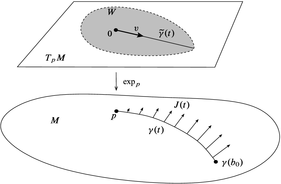
as above. The definition ensures that $\gamma (t)$ is not conjugate to $\gamma (0)$ for $t\in (0,b_0)$ , and therefore $\exp _p$ is a local diffeomorphism on some neighborhood of the set $L = \{tv: 0\le t < b_0\}$ . Let $W\subseteq T_pM$ be a convex open set containing L on which $\exp _p$ is a local diffeomorphism, and let $\tilde{g} = \exp _p ^*g$ , which is a Riemannian metric on W that satisfies the same curvature estimates as g (Fig. 11.2). By construction, W is a normal neighborhood of 0, and $\exp _p$ is a local isometry from $\big (W,\tilde{g}\big )$ to (M, g). The curve $\tilde{\gamma }(t) = tv$ for $t\in [0,b_0)$ is a radial geodesic in W, and Proposition 10.5 shows that the vector field $\tilde{J}(t) = d\big (\exp _p\big )_{tv}^{-1}(J(t))$ is a Jacobi field along $\tilde{\gamma }$ that vanishes at $$t=0$$

. Therefore, for $t\in (0,b_0)$ , the preceding argument implies that $\big |\tilde{J}(t)\big |_{\tilde{g}}\ge s_c(t) \big |\tilde{D}_t\tilde{J}(0)\big |_{\tilde{g}}$ in case (a) and $\big |\tilde{J}(t)\big |_{\tilde{g}}\le s_c(t) \big |\tilde{D}_t\tilde{J}(0)\big |_{\tilde{g}}$ in case (b). This implies that the conclusions of the theorem hold for J on the interval $$(0,b_0)$$

and thus by continuity on $$[0,b_0]$$

../images/56724_2_En_11_Chapter/56724_2_En_11_Fig2_HTML.png — Fig. 11.2:
Pulling the metric back to

$$T_pM$$ — Fig. 11.2:
Pulling the metric back to

To complete the proof, we need to show that $b_0\ge b_1$ in case (a) and $b_0\ge b_2$ in case (b). Assuming the hypothesis of (a), suppose for contradiction that $b_0{<}b_1$ . The only way this can occur is if $\gamma (b_0)$ is conjugate to $\gamma (0)$ along $\gamma$ , while $s_c(b_0){>}0$ . This means that there is a nontrivial normal Jacobi field $J\in \mathscr {J}(\gamma )$ satisfying $$J(0)=0=J(b_0)$$ . But the argument above showed that every such Jacobi field satisfies $|J(t)|\ge s_c(t) |D_tJ(0)|$ for $t\in [0,b_0]$ and thus $|J(b_0)|\ge s_c(b_0) |D_tJ(0)|>0$ , which is a contradiction. Similarly, in case (b), suppose $$b_0<b_2$$ . Then $$s_c(b_0)=0$$ , but $\gamma (b_0)$ is not conjugate to $\gamma (0)$ along $\gamma$ . If J is any nontrivial normal Jacobi field along $\gamma$ that vanishes at $$t=0$$ , the argument above shows that $|J(t)|\le s_c(t) |D_tJ(0)|$ for $t\in [0,b_0]$ , so $|J(b_0)|\le s_c(b_0) |D_tJ(0)|=0$ ; but this is impossible because $\gamma (b_0)$ is not conjugate to $\gamma (0)$ . $\square$

There is a generalization of the preceding theorem, called the Rauch comparison theorem, that allows for comparison of Jacobi fields in two different Riemannian manifolds when neither is assumed to have constant curvature. The statement and proof can be found in [CE08, Kli95].

Because all tangent vectors in a normal neighborhood are values of Jacobi fields along radial geodesics, the Jacobi field comparison theorem leads directly to the following comparison theorem for metrics.

Theorem 11.10

(Metric Comparison). Let (M, g) be a Riemannian manifold, and let $\big (U,\big (x^i\big )\big )$ be any normal coordinate chart for g centered at $p\in M$ . For each $c\in \mathbb {R}$ , let $$g_c$$ denote the constant-curvature metric on $U\smallsetminus \{p\}$ given in the same coordinates by formula (10.17).

(a)
Suppose all sectional curvatures of g are bounded above by a constant c. If $c\le 0$ , then for all $q\in U\smallsetminus \{p\}$ and all $w\in T_qM$ , we have $g(w,w)\ge g_c(w, w)$ . If , then the same holds, provided that $d_g(p, q)< \pi R$ .
(b)
If all sectional curvatures of g are bounded below by a constant c, then for all $q\in U\smallsetminus \{p\}$ and all $w\in T_qM$ , we have $g(w,w)\le g_c(w, w)$ .

Proof.

Let $q\in U\smallsetminus \{p\}$ , satisfying the restriction $d_g(p, q)< \pi R$ if we are in case (a) and $$c=1/R^2>0$$

, but otherwise arbitrary; and let $$b=d_g(p, q)$$

. Given $w\in T_qM$ , we can decompose w as a sum $$w = y+z$$

, where y is a multiple of the radial vector field $\partial _r$ and z is tangent to the level set $$r=b$$

. Then

by direct computation, and the Gauss lemma shows that $$g(y, z)=0$$

, so

$\begin{aligned} g(w,w)&= g(y,y) + g(z,z),\\ g_c(w,w)&= g_c(y,y) + g_c(z, z). \end{aligned}$

Because $\partial _r$ is a unit vector with respect to both g and $$g_c$$

, it follows that $$g(y,y) = g_c(y, y)$$

. So it suffices to prove the comparison for z.

There is a radial geodesic $\gamma :[0,b]\mathrel {\rightarrow }U$ satisfying $\gamma (0)=p$ and $\gamma (b)=q$ , and Corollary 10.11 shows that $$z=J(b)$$

for some Jacobi field J along $\gamma$ vanishing at $$t=0$$

, which is normal because it is orthogonal to $\gamma '$ at $$t=0$$

and

. Proposition 10.10 shows that J has the coordinate formula $J(t) = ta^i\partial _{i}|_{\gamma (t)}$ for some constants $\big (a^1,\dots , a^n\big )$ . Since the coordinates $\big (x^i )$ are normal coordinates for both g and $$g_c$$

, it follows that $\gamma$ is also a radial geodesic for $$g_c$$

, and the same vector field J is also a normal Jacobi field for $$g_c$$

along $\gamma$ . Therefore, $$g(z, z)=|J(b)|_g^2$$

and $g_c(z, z) = |J(b)|_{g_c}^2$ . In case (a), our hypothesis guarantees that $$s_c(b)>0$$

, so

../images/56724_2_En_11_Chapter/56724_2_En_11_Equ85_HTML.png

In case (b), the same argument with the inequalities reversed shows that $g(z,z)\le g_c(z, z)$ . $\square$

The next three comparison theorems (Laplacian, conjugate point, and volume comparisons) can be proved equally easily under the assumption of either an upper bound or a lower bound for the sectional curvature, just like the preceding theorems. However, we state these only for the case of an upper bound, because we will prove stronger theorems later in the chapter based on lower bounds for the Ricci curvature (see Thms. 11.15, 11.16, and 11.19).

The first of the three is a comparison of the Laplacian of the radial distance function with its constant-curvature counterpart. Our primary interest in the Laplacian of the distance function stems from its role in volume and conjugate point comparisons (see Thms. 11.14, 11.16, and 11.19 below); but it also plays an important role in the study of various partial differential equations on Riemannian manifolds.

Theorem 11.11

(Laplacian Comparison I). Suppose (M, g) is a Riemannian n-manifold whose sectional curvatures are all bounded above by a constant c. Suppose $p\in M$ , U is a normal neighborhood of p, r is the radial distance function on U, and $$s_c$$

is defined as in Proposition 11.3. Then on $U_0\smallsetminus \{p\}$ , we have

$\begin{aligned} \Delta r \ge (n-1)\frac{s_c'(r)}{s_c(r)}, \end{aligned}$

where

if $c\le 0$ , while $U_0 = \{q\in U: r(q)<\pi R\}$ if $$c=1/R^2>0$$

Proof.

By the result of Problem 5-14, $\Delta r = {{\,\mathrm{tr}\,}}_g \big (\nabla ^2 r\big ) = {{\,\mathrm{tr}\,}}\big (\mathscr {H}_r\big )$ . The result then follows from the Hessian comparison theorem, using the fact that ${{\,\mathrm{tr}\,}}(\pi _r) = n-1$ , which can be verified easily by expressing $\pi _r$ locally in an adapted orthonormal frame for the r-level sets. $\square$

The next theorem shows how an upper curvature bound prevents the formation of conjugate points. It will play a decisive role in the proof of the Cartan–Hadamard theorem in the next chapter.

Theorem 11.12

(Conjugate Point Comparison I). Suppose (M, g) is a Riemannian n-manifold whose sectional curvatures are all bounded above by a constant c. If $c\le 0$ , then no point of M has conjugate points along any geodesic. If $$c=1/R^2>0$$ , then there is no conjugate point along any geodesic segment shorter than $\pi R$ .

Proof.

The case $c\le 0$ is covered by Problem 10-7, so assume $$c=1/R^2>0$$ . Let $\gamma :[0,b]\mathrel {\rightarrow }M$ be a unit-speed geodesic segment, and suppose J is a nontrivial normal Jacobi field along $\gamma$ that vanishes at $$t=0$$ . The Jacobi field comparison theorem implies that $|J(t)|\ge (\text {constant})\sin (t/R)>0$ as long as $0<t<\pi R$ . $\square$

The last of our sectional curvature comparison theorems is a comparison of volume growth of geodesic balls. Before proving it, we need the following lemma, which shows how the Riemannian volume form is related to the Laplacian of the radial distance function.

Lemma 11.13.

Suppose (M, g) is a Riemannian manifold and $\big (x^i\big )$ are Riemannian normal coordinates on a normal neighborhood U of $p\in M$ . Let $\det g$ denote the determinant of the matrix $(g_{ij})$ in these coordinates, let r be the radial distance function, and let $\partial _r$ be the unit radial vector field. The following identity holds on $U\smallsetminus \{p\}$ :

$\begin{aligned} \Delta r =\partial _r \log \big ( r^{n-1}\sqrt{\det g} \big ). \end{aligned}$

(11.23)

Proof.

Corollary 6.10 to the Gauss lemma shows that the vector fields ${{\,\mathrm{grad}\,}}r$ and $\partial _r$ are equal on $U\smallsetminus \{p\}$ . Comparing the components of these two vector fields in normal coordinates, we conclude (using the summation convention as usual) that

$\begin{aligned} g^{ij} \partial _j r= \frac{x^i}{r} . \end{aligned}$

Based on the formula for $\Delta r$ from Proposition 2.46, we compute

$\begin{aligned} \Delta r&= \frac{1}{\sqrt{\det g}} \partial _i \left( g^{ij} \sqrt{\det g} \,\partial _j r\right) \\&= \frac{1}{\sqrt{\det g}} \partial _i \left( \frac{x^i}{r} \sqrt{\det g} \right) \\&= \partial _i \left( \frac{x^i}{r} \right) + \frac{1}{\sqrt{\det g}}\frac{x^i}{r} \partial _i \sqrt{\det g} \\&= \frac{n-1}{r} + \frac{1}{\sqrt{\det g}} \partial _r \sqrt{\det g}, \end{aligned}$

where the first term in the last line follows by direct computation using $r =\big ( \sum _i\big (x^i\big )^2\big )^{1/2}$ . This is equivalent to (11.23). $\square$

The following result was proved by Paul Günther in 1960 [Gün60]. (Günther also proved an analogous result in the case of a lower sectional curvature bound, but that result has been superseded by the Bishop–Gromov theorem, Thm. 11.19 below.)

Theorem 11.14

(Günther’s Volume Comparison). Suppose (M, g) is a connected Riemannian n-manifold whose sectional curvatures are all bounded above by a constant c. Given $p\in M$ , let $\delta _0 = \text {inj}(p)$ if $c\le 0$ , and $\delta _0 = \min (\pi R,\text {inj}(p))$ if $$c=1/R^2>0$$

. For every positive number $\delta \le \delta _0$ , let $V_g(\delta )$ denote the volume of the geodesic ball $B_\delta (p)$ in (M, g), and let $V_c(\delta )$ denote the volume of a geodesic ball of radius $\delta$ in the n-dimensional Euclidean space, hyperbolic space, or sphere with constant sectional curvature c. Then for every $0<\delta \le \delta _0$ , we have

$\begin{aligned} V_g(\delta ) \ge V_c(\delta ), \end{aligned}$

(11.24)

and the quotient $V_g(\delta )/V_c(\delta )$ is a nondecreasing function of $\delta$ that approaches 1 as $\delta \searrow 0$ . If equality holds in (11.24) for some $\delta \in (0,\delta _0]$ , then g has constant sectional curvature c on the entire geodesic ball $B_{\delta }(p)$ .

Proof.

The volume estimate (11.24) follows easily from the metric comparison theorem, which implies that the determinants of the metrics g and $$g_c$$ in normal coordinates satisfy $\sqrt{\det g} \ge \sqrt{\det g_c}$ . If that were all we needed, we could stop here; but to prove the other statements, we need a more involved argument, which incidentally provides another proof of (11.24) that does not rely directly on the metric comparison theorem, and therefore can be adapted more easily to the case in which we have only an estimate of the Ricci curvature (see Thm. 11.19 below).

Let $\big (x^i\big )$ be normal coordinates on $B_{\delta _0}(p)$ (interpreted as all of M if $\delta _0=\infty$ ). Using these coordinates, we might as well consider g to be a Riemannian metric on an open subset of $\mathbb {R}^n$ and p to be the origin. Let ${\bar{g}}$ denote the Euclidean metric in these coordinates, and let $$g_c$$ denote the constant-curvature metric in the same coordinates, given on the complement of the origin by (10.17).

The Laplacian comparison theorem together with Lemma 11.13 shows that

$\begin{aligned} \partial _r \log \big ( r^{n-1}\sqrt{\det g} \big ) = \Delta r \ge (n-1)\frac{s_c'(r)}{s_c(r)} = \partial _r \log \big (s_c(r)^{n-1}\big ). \end{aligned}$

(11.25)

Thus $\log \big ( r^{n-1}\sqrt{\det g} / s_c(r)^{n-1}\big )$ is a nondecreasing function of r along each radial geodesic, and so is the ratio $r^{n-1}\sqrt{\det g} / s_c(r)^{n-1}$ . To compute the limit as $r\searrow 0$ , note that $g_{ij} = \delta _{ij}$ at the origin, so $\sqrt{\det g}$ converges uniformly to 1 as $r\searrow 0$ . Also, for every c, we have $s_c(r)/r\mathrel {\rightarrow }1$ as $r\searrow 0$ , so $r^{n-1}\sqrt{\det g} / s_c(r)^{n-1}\mathrel {\rightarrow }1$ .

We can write $dV_g = \sqrt{\det g}\, dV_{{\bar{g}}}$ . Corollary 10.17 in the case $$c=0$$

shows that

$\begin{aligned} V_g(\delta ) =\int _{\mathbb {S}^{n-1}} \int _0^\delta \big (\sqrt{\det g}\big )\circ \Phi (\rho ,\omega )\rho ^{n-1}\,d\rho \, dV_{\mathring{g}}, \end{aligned}$

where $\Phi (\rho ,\omega ) = \rho \omega$ for $\rho \in (0,\delta _0)$ and $\omega \in \mathbb {S}^{n-1}$ . The same corollary shows that

$\begin{aligned} V_c(\delta ) =\int _{\mathbb {S}^{n-1}} \int _0^\delta s_c(\rho )^{n-1}\,d\rho \, dV_{\mathring{g}} = \left( \int _0^\delta s_c(\rho )^{n-1}\, d\rho \right) \left( \int _{\mathbb {S}^{n-1}} dV_{\mathring{g}}\right) . \end{aligned}$

Therefore,

../images/56724_2_En_11_Chapter/56724_2_En_11_Equ26_HTML.png

(11.26)

where we have written

$\begin{aligned} \lambda (\rho ,\omega ) = \frac{\big (\sqrt{\det g}\big )\circ \Phi (\rho ,\omega )\rho ^{n-1}}{s_c(\rho )^{n-1}}. \end{aligned}$

The argument above (together with the fact that $r\circ \Phi = \rho$ ) shows that $\lambda (\rho ,\omega )$ is a nondecreasing function of $\rho$ for each $\omega$ , which approaches 1 uniformly as $\rho \searrow 0$ .

We need to show that the quotient in parentheses in the last line of (11.26) is also nondecreasing as $\delta$ increases. Suppose $0<\delta _1<\delta _2$ . Because $\lambda$ is nondecreasing, we have

$\begin{aligned} \int _0^{\delta _1} \lambda (\rho ,\omega ) s_c(\rho )^{n-1}\, d\rho&\int _{\delta _1}^{\delta _2} s_c(\rho )^{n-1}\, d\rho \\&\le \left( \int _0^{\delta _1}s_c(\rho )^{n-1}\, d\rho \right) \lambda (\delta _1,\omega ) \left( \int _{\delta _1}^{\delta _2} s_c(\rho )^{n-1}\, d\rho \right) \\&\le \int _0^{\delta _1}s_c(\rho )^{n-1}\, d\rho \int _{\delta _1}^{\delta _2}\lambda (\rho ,\omega ) s_c(\rho )^{n-1}\, d\rho , \end{aligned}$

and therefore (suppressing the dependence of the integrands on $\rho$ and $\omega$ for brevity),

$\begin{aligned} \int _0^{\delta _1} \lambda s_c^{n-1}\, d\rho&\int _{0}^{\delta _2} s_c^{n-1}\, d\rho \\&= \int _0^{\delta _1} \lambda s_c^{n-1}\, d\rho \left( \int _{0}^{\delta _1} s_c^{n-1}\, d\rho + \int _{\delta _1}^{\delta _2} s_c^{n-1}\, d\rho \right) \\&\le \int _0^{\delta _1} \lambda s_c^{n-1}\, d\rho \int _{0}^{\delta _1} s_c^{n-1}\, d\rho + \int _0^{\delta _1} s_c^{n-1}\, d\rho \int _{\delta _1}^{\delta _2} \lambda s_c^{n-1}\, d\rho \\&= \int _0^{\delta _1} s_c^{n-1}\, d\rho \int _{0}^{\delta _2} \lambda s_c^{n-1}\, d\rho . \end{aligned}$

Evaluating (11.26) at $\delta _1$ and $\delta _2$ and inserting the inequality above shows that the ratio ${{\,\mathrm{Vol}\,}}_g(\delta )/{{\,\mathrm{Vol}\,}}_c(\delta )$ is nondecreasing as a function of $\delta$ , and it approaches 1 as $\delta \searrow 0$ because $\lambda (\rho ,\omega )\mathrel {\rightarrow }1$ as $\rho \searrow 0$ . It follows that $V_g(\delta )\ge V_c(\delta )$ for all $\delta \in (0,\delta _0]$ .

It remains only to consider the case in which the volume ratio is equal to 1 for some $\delta$ . If $\lambda (\rho ,\omega )$ is not identically 1 on the set where $0<\rho <\delta$ , then it is strictly greater than 1 on a nonempty open subset, which implies that the volume ratio in (11.26) is strictly greater than 1; so ${{\,\mathrm{Vol}\,}}_g(\delta ) = {{\,\mathrm{Vol}\,}}_c(\delta )$ implies $\lambda (\rho ,\omega )\equiv 1$ on $(0,\delta )\times \mathbb {S}^{n-1}$ , and pulling back to U via $\Phi ^{-1}$ shows that $r^{n-1}\sqrt{\det g} \equiv s_c(r)^{n-1}$ on $B_\delta (p)$ . By virtue of (11.25), we have $\Delta r \equiv (n-1) s_c'(r)/s_c(r)$ , or in other words, ${{\,\mathrm{tr}\,}}(\mathscr {H}_r) = {{\,\mathrm{tr}\,}}((s_c'(r)/s_c(r))\pi _r)$ . It follows from the Hessian comparison theorem that the endomorphism field $\mathscr {H}_r-\left( s_c'(r)/s_c(r)\right) \pi _r$ is positive semidefinite, so its eigenvalues are all nonnegative. Since its trace is zero, the eigenvalues must all be zero. In other words, $\mathscr {H}_r \equiv (s_c'(r)/s_c(r))\pi _r$ on the geodesic ball $B_\delta (p)$ . It then follows from Proposition 11.3 that g has constant sectional curvature c on that ball. $\square$

Comparisons Based on Ricci Curvature

All of our comparison theorems so far have been based on assuming an upper or lower bound for the sectional curvature. It is natural to wonder whether anything can be said if we weaken the hypotheses and assume only bounds on other curvature quantities such as Ricci or scalar curvature.

It should be noted that except in very low dimensions, assuming a bound on Ricci or scalar curvature is a strictly weaker hypothesis than assuming one on sectional curvature. Recall Proposition 8.32, which says that on an n-dimensional Riemannian manifold, the Ricci curvature evaluated on a unit vector is a sum of $$n-1$$ sectional curvatures, and the scalar curvature is a sum of $$n(n-1)$$ sectional curvatures. Thus if (M, g) has sectional curvatures bounded below by c, then its Ricci curvature satisfies $Rc (v, v)\ge (n-1)c$ for all unit vectors v, and its scalar curvature satisfies $S \ge n(n-1)c$ , with analogous inequalities if the sectional curvature is bounded above. However, the converse is not true: an upper or lower bound on the Ricci curvature implies nothing about individual sectional curvatures, except in dimensions 2 and 3, where the entire curvature tensor is determined by the Ricci curvature (see Cors. 7.26 and 7.27). For example, in every even dimension greater than or equal to 4, there are compact Riemannian manifolds called Calabi–Yau manifolds that have zero Ricci curvature but nonzero sectional curvatures (see, for example, [[Bes87], Chap. 11]).

In this section we investigate the extent to which bounds on the Ricci curvature lead to useful comparison theorems. The strongest theorems of the preceding section, such as the Hessian, Jacobi field, and metric comparison theorems, do not generalize to the case in which we merely have bounds on Ricci curvature. However, it is a remarkable fact that Laplacian, conjugate point, and volume comparison theorems can still be proved assuming only a lower (but not upper) bound on the Ricci curvature. (The problem of drawing global conclusions from scalar curvature bounds is far more subtle, and we do not pursue it here. A good starting point for learning about that problem is [Bes87].)

The next theorem is the analogue of Theorem 11.11.

Theorem 11.15

(Laplacian Comparison II). Let (M, g) be a Riemannian n-manifold, and suppose there is a constant c such that the Ricci curvature of M satisfies $Rc (v, v)\ge (n-1)c$ for all unit vectors v. Given any point $p\in M$ , let U be a normal neighborhood of p and let r be the radial distance function on U. Then the following inequality holds on $U_0\smallsetminus \{p\}$ :

$\begin{aligned} \Delta r \le (n-1)\frac{s_c'(r)}{s_c(r)}, \end{aligned}$

(11.27)

where

is defined by (10.8), and $$U_0=U$$

if $c\le 0$ , while $U_0 = \{q\in U: r(q)<\pi R\}$ if $$c=1/R^2>0$$

Proof.

Let $q\in U_0\smallsetminus \{p\}$ be arbitrary, and let $\gamma :[0,b]\mathrel {\rightarrow }U_0$ be the unit-speed radial geodesic from p to q. We will show that (11.27) holds at $\gamma (t)$ for $0<t\le b$ .

Because covariant differentiation commutes with the trace operator (since it is just a particular kind of contraction), the Riccati equation (11.7) for $\mathscr {H}_r$ implies the following scalar equation along $\gamma$ for $\Delta r = {{\,\mathrm{tr}\,}}\big (\mathscr {H}_r\big )$ :

$\begin{aligned} \frac{d}{dt}\Delta r + {{\,\mathrm{tr}\,}}\big (\mathscr {H}_r^2\big ) + {{\,\mathrm{tr}\,}}R_{\gamma '} = 0. \end{aligned}$

(11.28)

We need to analyze the last two terms on the left-hand side. We begin with the last term. In terms of any local orthonormal frame $$(E_i)$$

, we have

$\begin{aligned} {{\,\mathrm{tr}\,}}R_{\gamma '}&= \sum _{i=1}^n \left\langle R_{\gamma '}(E_i), E_i\right\rangle =\sum _{i=1}^n \left\langle R(E_i,\gamma ')\gamma ', E_i\right\rangle =\sum _{i=1}^n Rm (E_i,\gamma ',\gamma ', E_i)\\&= Rc (\gamma ',\gamma '). \end{aligned}$

To analyze the $\mathscr {H}_r^2$ term, let us set

$\begin{aligned} \smash [t]{\mathring{\mathscr {H}}}_r = \mathscr {H}_r - \frac{\Delta r}{n-1} \pi _r. \end{aligned}$

(11.29)

We compute

$\begin{aligned} {{\,\mathrm{tr}\,}}\big (\smash [t]{\mathring{\mathscr {H}}}_r^2\big )&= {{\,\mathrm{tr}\,}}\big (\mathscr {H}_r^2\big )-\frac{\Delta r}{n-1}{{\,\mathrm{tr}\,}}(\mathscr {H}_r\circ \pi _r)- \frac{\Delta r}{n-1} {{\,\mathrm{tr}\,}}(\pi _r\circ \mathscr {H}_r) + \frac{(\Delta r)^2}{(n-1)^2}{{\,\mathrm{tr}\,}}\left( \pi _r^2\right) . \end{aligned}$

To simplify this, note that $\pi _r^2=\pi _r$ because $\pi _r$ is a projection, and thus ${{\,\mathrm{tr}\,}}\left( \pi _r^2\right) ={{\,\mathrm{tr}\,}}(\pi _r) = n-1$ . Also, $\mathscr {H}_r(\partial _r) \equiv 0$ implies that $\mathscr {H}_r\circ \pi _r = \mathscr {H}_r$ ; and since $\mathscr {H}_r$ is self-adjoint, $\left\langle \mathscr {H}_r v,\partial _r\right\rangle _g = \left\langle v, \mathscr {H}_r\partial _r\right\rangle _g = 0$ for all v, so the image of $\mathscr {H}_r$ is contained in the orthogonal complement of $\partial _r$ , and it follows that $\pi _r \circ \mathscr {H}_r = \mathscr {H}_r$ as well. Thus the last three terms in the formula for ${{\,\mathrm{tr}\,}}\big (\smash [t]{\mathring{\mathscr {H}}}_r^2\big )$ combine to yield

$\begin{aligned} {{\,\mathrm{tr}\,}}\big (\smash [t]{\mathring{\mathscr {H}}}_r^2\big ) = {{\,\mathrm{tr}\,}}\big (\mathscr {H}_r^2\big ) - \frac{(\Delta r)^2}{n-1}. \end{aligned}$

Solving this for ${{\,\mathrm{tr}\,}}\big (\mathscr {H}_r^2\big )$ , substituting into (11.28), and dividing by $$n-1$$

, we obtain

$\begin{aligned} \frac{d}{dt}\left( \frac{\Delta r}{n-1}\right) + \left( \frac{\Delta r}{n-1}\right) ^2 + \frac{{{\,\mathrm{tr}\,}}\big (\smash [t]{\mathring{\mathscr {H}}}_r^2\big ) + Rc (\gamma ',\gamma ') }{n-1}= 0. \end{aligned}$

(11.30)

Let

, so that

$\begin{aligned} H'(t) + H(t)^2 + c \equiv 0. \end{aligned}$

We wish to apply the $1\times 1$ case of the matrix Riccati comparison theorem (Thm. 11.6) with H(t) as above, $S(t) \equiv c$ ,

$\begin{aligned} \tilde{H}(t) = \frac{(\Delta r)\big |_{\gamma (t)}}{n-1}, \quad \text {and} \quad \tilde{S}(t) = \frac{{{\,\mathrm{tr}\,}}\big (\smash [t]{\mathring{\mathscr {H}}}_r^2\big )\big |_{\gamma (t)} + Rc (\gamma '(t),\gamma '(t)) }{n-1}. \end{aligned}$

Note that $\smash [t]{\mathring{\mathscr {H}}}_r^2$ is positive semidefinite, which means that all of its eigenvalues are nonnegative, so its trace (which is the sum of the eigenvalues) is also nonnegative. (This is the step that does not work in the case of an upper bound on Ricci curvature.) Thus our hypothesis on the Ricci curvature guarantees that $\tilde{S}(t) \ge c$ for all $t\in (0,b]$ .

To apply Theorem 11.6, we need to verify that $\tilde{S}$ has a continuous extension to [0, b] and that $\tilde{H}(t) - H(t)$ has a nonnegative limit as $t\searrow 0$ . Recall that we showed in (11.19) and (11.20) that $$s_c'(r)/s_c(r)= 1/r + O(r)$$ and $\mathscr {H}_r = (1/r) \pi _r + O(r)$ as $r\searrow 0$ . This implies that $\Delta r = {{\,\mathrm{tr}\,}}(\mathscr {H}_r) = (n-1)/r + O(r)$ , and therefore both $\smash [t]{\mathring{\mathscr {H}}}_r|_{\gamma (t)}$ and $\tilde{H} (t)-H(t)$ approach 0 and $\tilde{S}(t)$ approaches ${ Rc (\gamma '(0),\gamma '(0))/(n-1)} \ge c$ as $t\searrow 0$ . Therefore, we can apply Theorem 11.6 to conclude that $\tilde{H}(t) \le H(t)$ for $t\in (0,b]$ . Since $\gamma (b)=q$ was arbitrary, this completes the proof. $\square$

The next theorem and its two corollaries will be crucial ingredients in the proofs of our theorems in the next chapter about manifolds with positive Ricci curvature (see Thms. 12.28 and 12.24).

Theorem 11.16

(Conjugate Point Comparison II). Let (M, g) be a Riemannian n-manifold, and suppose there is a positive constant $$c = 1/R^2$$ such that the Ricci curvature of M satisfies $Rc (v, v)\ge (n-1)c$ for all unit vectors v. Then every geodesic segment of length at least $\pi R$ has a conjugate point.

Proof.

Let U be a normal neighborhood of an arbitrary point $p\in M$ . The second Laplacian comparison theorem (Thm. 11.15) combined with Lemma 11.13 shows that

$\begin{aligned} \partial _r \log \big ( r^{n-1}\sqrt{\det g} \big ) = \Delta r \le (n-1)\frac{s_c'(r)}{s_c(r)} = \partial _r \log \big (s_c(r)^{n-1}\big ) \end{aligned}$

on the subset $U_0\subseteq U$ where $r<\pi R$ . Since $r^{n-1}\sqrt{\det g} / s_c(r)^{n-1}\mathrel {\rightarrow }1$ as $r\searrow 0$ , this implies that $r^{n-1}\sqrt{\det g} / s_c(r)^{n-1}\le 1$ everywhere in $$U_0$$

, or equivalently,

$\begin{aligned} \sqrt{\det g}\le s_c(r)^{n-1}/r^{n-1}. \end{aligned}$

(11.31)

Suppose U contains a point q where $r\ge \pi R$ , and let $\gamma :[0,b]\mathrel {\rightarrow }U$ be the unit-speed radial geodesic from p to q. Because $s_c(\pi R)=0$ , (11.31) shows that $\det g(\gamma (t)) \mathrel {\rightarrow }0$ as $t\nearrow \pi R$ , and therefore by continuity $\det g=0$ at $\gamma (b)$ , which contradicts the fact that $\det g>0$ in every coordinate neighborhood. The upshot is that no normal neighborhood can include points where $r\ge \pi R$ .

Now suppose $\gamma :[0,b]\mathrel {\rightarrow }M$ is a unit-speed geodesic with $b\ge \pi R$ , and assume for the sake of contradiction that $\gamma$ has no conjugate points. Let $p{=}\gamma (0)$ and $v{=}\gamma '(0)$ , so $\gamma (t) = \exp _p(tv)$ for $t\in [0,b]$ . As in the proof of Theorem 11.9, because $\gamma$ has no conjugate points, we can choose a star-shaped open subset $W\subseteq T_pM$ containing the set $L = \{tv: 0\le t < b_0\}\subseteq T_pM$ on which $\exp _p$ is a local diffeomorphism, and let $\tilde{g}$ be the pulled-back metric $\exp _p ^*g$ on W, which satisfies the same curvature estimates as g. Then $\tilde{\gamma }(t) = tv$ is a radial $\tilde{g}$ -geodesic in W of length greater than or equal to $\pi R$ , which contradicts the argument in the preceding paragraph. $\square$

Corollary 11.17

(Injectivity Radius Comparison). Let (M, g) be a Riemannian n-manifold, and suppose there is a positive constant $$c=1/R^2$$ such that the Ricci curvature of M satisfies $Rc (v, v)\ge (n-1)c$ for all unit vectors v. Then for every point $p\in M$ , we have $\text {inj}(p)\le \pi R$ .

Proof.

Every radial geodesic segment in a geodesic ball is minimizing, but the preceding theorem shows that no geodesic segment of length $\pi R$ or greater is minimizing. Thus no geodesic ball has radius greater than $\pi R$ . $\square$

Corollary 11.18

(Diameter Comparison). Let (M, g) be a complete, connected Riemannian n-manifold, and suppose there is a positive constant $$c=1/R^2$$ such that the Ricci curvature of M satisfies $Rc (v, v)\ge (n-1)c$ for all unit vectors v. Then the diameter of M is less than or equal to $\pi R$ .

Proof.

This follows from the fact that any two points of M can be connected by a minimizing geodesic segment, and the conjugate point comparison theorem implies that no such segment can have length greater than $\pi R$ . $\square$

Our final comparison theorem is a powerful volume estimate under the assumption of a lower bound on the Ricci curvature. We will use it in the proof of Theorem 12.28 in the next chapter, and it plays a central role in many of the more advanced results of Riemannian geometry.

A weaker version of this result was proved by Paul Günther in 1960 [Gün60] for balls within the injectivity radius under the assumption of a lower bound on sectional curvature; it was improved by Richard L. Bishop in 1963 (announced in [Bis63], with a proof in [BC64]) to require only a lower Ricci curvature bound; and then it was extended by Misha Gromov in 1981 [Gro07] to cover all metric balls in the complete case, not just those inside the injectivity radius.

Theorem 11.19

(Bishop–Gromov Volume Comparison). Let (M, g) be a connected Riemannian n-manifold, and suppose there is a constant c such that the Ricci curvature of M satisfies $Rc (v, v)\ge (n-1)c$ for all unit vectors v. Let $p\in M$ be given, and for every positive number $\delta$ , let $V_g(\delta )$ denote the volume of the metric ball of radius $\delta$ about p in (M, g), and let $V_c(\delta )$ denote the volume of a metric ball of radius $\delta$ in the n-dimensional Euclidean space, hyperbolic space, or sphere with constant sectional curvature c. Then for every $0<\delta \le \text {inj}(p)$ , we have

$\begin{aligned} V_g(\delta ) \le V_c(\delta ), \end{aligned}$

(11.32)

and the quotient $V_g(\delta )/V_c(\delta )$ is a nonincreasing function of $\delta$ that approaches 1 as $\delta \searrow 0$ . If (M, g) is complete, the same is true for all positive $\delta$ , not just $\delta \le \text {inj}(p)$ . In either case, if equality holds in (11.32) for some $\delta$ , then g has constant sectional curvature on the entire metric ball of radius $\delta$ about p.

Proof.

First consider $\delta \le \text {inj}(p)$ , in which case a metric ball of radius $\delta$ in M is actually a geodesic ball. With the exception of the first and last paragraphs, the proof of Theorem 11.14 goes through with all of the inequalities reversed, and with the first Laplacian comparison theorem replaced by its counterpart Theorem 11.15, to show that $V_g(\delta )/V_c(\delta )$ is a nonincreasing function of $\delta$ that approaches 1 as $\delta \searrow 0$ , and (11.32) follows.

In case M is complete, $\exp _p$ is defined and smooth on all of $$T_pM$$

. Theorem 10.34 shows that ${{\,\mathrm{Cut}\,}}(p)$ has measure zero in M and $\exp _p$ maps the open subset ${{\,\mathrm{ID}\,}}(p)\subseteq T_pM$ diffeomorphically onto the complement of ${{\,\mathrm{Cut}\,}}(p)$ in M. Therefore, for every $\delta >0$ , the metric ball of radius $\delta$ is equal to $\exp _p\big (B_\delta (0)\cap {{\,\mathrm{ID}\,}}(p)\big )$ up to a set of measure zero, where $B_\delta (0)$ denotes the $\delta$ -ball about 0 in $$T_pM$$

. Using an orthonormal basis to identify $$(T_pM, g_p)$$

with $(\mathbb {R}^n,{\bar{g}})$ , we can compute the volume of a metric $\delta$ -ball as

$\begin{aligned} V_g(\delta ) = \int _{{{\,\mathrm{ID}\,}}(p)\cap B_\delta (0)} \exp _p^* dV_g = \int _{{{\,\mathrm{ID}\,}}(p)\cap B_\delta (0)} \sqrt{\det g}\, dV_{\bar{g}}, \end{aligned}$

where $\det g$ denotes the determinant of the matrix of g in the normal coordinates determined by the choice of basis.

Let $\Phi :\mathbb {R}^+\times \mathbb {S}^{n-1}\mathrel {\rightarrow }T_pM\smallsetminus \{0\}\cong \mathbb {R}^n\smallsetminus \{0\}$ be the map $\Phi (\rho ,\omega ) = \rho \omega$ as in Corollary 10.17, and define $\tilde{s}_c:\mathbb {R}^+\mathrel {\rightarrow }[0,\infty )$ by $\tilde{s}_c(\rho ) = s_c(\rho )$ if $c\le 0$ , while in the case $$c=1/R^2>0$$

../images/56724_2_En_11_Chapter/56724_2_En_11_Equ86_HTML.png

Corollary 11.18 shows that the cut time of every unit vector in $$T_pM$$

is less than or equal to $\pi R$ . Thus $\tilde{s}_c(\rho )>0$ whenever $\Phi (\rho ,\omega )\in {{\,\mathrm{ID}\,}}(p)$ , and we can define $\tilde{\lambda }:\mathbb {R}^+\times \mathbb {S}^{n-1}\mathrel {\rightarrow }\mathbb {R}$ by

../images/56724_2_En_11_Chapter/56724_2_En_11_Equ87_HTML.png

and just as in the proof of Theorem 11.14, we can write

$\begin{aligned} V_g(\delta )&=\int _{\mathbb {S}^{n-1}} \int _0^\delta \tilde{\lambda }(\rho ,\omega ) \tilde{s}_c(\rho )^{n-1}\,d\rho \, dV_{\mathring{g}},\\ V_c(\delta )&=\int _{\mathbb {S}^{n-1}} \int _0^\delta \tilde{s}_c(\rho )^{n-1}\,d\rho \, dV_{\mathring{g}}. \end{aligned}$

The arguments of Theorem 11.14 (with inequalities reversed) show that for each $\omega \in \mathbb {S}^{n-1}$ , the function $\tilde{\lambda }(\rho ,\omega )$ is nonincreasing in $\rho$ for all positive $\rho$ , and it follows just as in that proof that $V_g(\delta )/V_c(\delta )$ (now interpreted as a ratio of volumes of metric balls) is nonincreasing for all $\delta >0$ and approaches 1 as $\delta \searrow 0$ , and (11.32) follows.

Finally, suppose $V_g(\delta ) = V_c(\delta )$ for some $\delta >0$ , and assume first that $\delta \le \text {inj}(p)$ . An argument exactly analogous to the one at the end of the proof of Theorem 11.14 shows that $\lambda (\rho ,\omega )\equiv 1$ everywhere on the set where $0<\rho <\delta$ . Combined with Lemma 11.13, this implies that

$\begin{aligned} \Delta r = (n-1)\frac{s_c'(r)}{s_c(r)} \end{aligned}$

(11.33)

everywhere on $B_\delta (p)\smallsetminus \{p\}$ . This means that along each unit-speed radial geodesic $\gamma$ , the function $u(t) = (\Delta r)|_{\gamma (t)}/(n-1) = s_c'(t)/s_c(t)$ satisfies $u' + u^2 + c \equiv 0$ by direct computation. Comparing this to (11.30), we conclude that

$\begin{aligned} \frac{{{\,\mathrm{tr}\,}}\big (\smash [t]{\mathring{\mathscr {H}}}_r^2\big ) + Rc (\gamma ',\gamma ') }{n-1}\equiv c \end{aligned}$

on $B_\delta (p)\smallsetminus \{p\}$ . Since ${{\,\mathrm{tr}\,}}\big (\smash [t]{\mathring{\mathscr {H}}}_r^2\big )\ge 0$ and $Rc (\gamma ',\gamma ') \ge (n-1)c$ everywhere, this is possible only if ${{\,\mathrm{tr}\,}}\big (\smash [t]{\mathring{\mathscr {H}}}_r^2\big )$ vanishes identically there. Because $\smash [t]{\mathring{\mathscr {H}}}_r^2$ is positive semidefinite and its trace is zero, it must vanish identically, which by definition of $\smash [t]{\mathring{\mathscr {H}}}_r$ means

$\begin{aligned} \mathscr {H}_r = \frac{\Delta r}{n-1} \pi _r = \frac{s_c'(r)}{s_c(r)}\pi _r. \end{aligned}$

Proposition 11.3 then shows that g has constant sectional curvature c on $B_\delta (p)$ .

Now suppose (M, g) is complete. The argument of Theorem 11.14 then shows that $\tilde{\lambda }(\rho ,\omega )\equiv 1$ everywhere on the set where $0<\rho <\delta$ and $\tilde{s}_c(\rho )>0$ . In view of the definition of $\tilde{\lambda }$ , this implies in particular that ${{\,\mathrm{ID}\,}}(p)\cap B_\delta (0)$ contains all of the points in $B_\delta (0)$ where $\tilde{s}_c(r)>0$ . In case $c\le 0$ , $\tilde{s}_c(r)=s_c(r)>0$ everywhere, so ${{\,\mathrm{ID}\,}}(p)\cap B_\delta (0)=B_\delta (0)$ and therefore the metric ball of radius $\delta$ around p is actually a geodesic ball, and the argument above applies.

In case $$c=1/R^2>0$$ , if $\delta \le \pi R$ , then $\tilde{s}_c(r)=s_c(r)>0$ on $B_\delta (0)$ , and once again we conclude that the metric $\delta$ -ball is a geodesic ball. On the other hand, if $\delta >\pi R$ , then the diameter comparison theorem (Cor. 11.18) shows that the metric ball of radius $\delta$ is actually the entire manifold. The fact that the volume ratio is nonincreasing implies that $V_g(\pi R)= V_c(\pi R)$ , and the argument above shows that g has constant sectional curvature c on the metric ball of radius $\pi R$ . Since the closure of that ball is all of M, the result follows by continuity. $\square$

The next corollary is immediate.

Corollary 11.20.

Suppose (M, g) is a compact Riemannian manifold and there is a positive constant $$c=1/R^2$$ such that the Ricci curvature of M satisfies $Rc (v, v)\ge {(n-1)c}$ for all unit vectors v. Then the volume of M is no greater than the volume of the n-sphere of radius R with its round metric, and if equality holds, then (M, g) has constant sectional curvature c. $\square$

(For explicit formulas for the volumes of n-spheres, see Problem 10-4.)

Problems

11-1.
Let (M, g) be a Riemannian manifold, and let U be a normal neighborhood of $p\in M$ . Use Corollary 6.42 to show that in every choice of polar normal coordinates $\big (\theta ^1,\dots ,\theta ^{n-1}, r\big )$ on a subset of $U\smallsetminus \{p\}$ (see Example 6.45), the covariant Hessian of r is given by
$\begin{aligned} \nabla ^2 r = \frac{1}{2} \sum _{\alpha ,\beta =1}^{n-1} \big (\partial _r g_{\alpha \beta }\big ) d\theta ^\alpha \, d\theta ^\beta . \end{aligned}$
11-2.
Prove the following extension to Proposition 11.2: Suppose P is an embedded submanifold of a Riemannian manifold (M, g), U is a normal neighborhood of P in M, and r is the radial distance function for P in U (see Prop. 6.37). If $\gamma :[0,b]\mathrel {\rightarrow }U$ is a geodesic segment with $\gamma (0)\in P$ and $\gamma '(0)$ normal to P, and J is a Jacobi field along $\gamma$ that is transverse to P in the sense of Problem 10-14, then $D_tJ(t) = \mathscr {H}_r(J(t))$ for all $t\in [0,b]$ .
11-3.
Let (M, g) be a Riemannian manifold, and let f be any smooth local distance function defined on an open subset $U\subseteq M$ . Let $F = {{\,\mathrm{grad}\,}}f$ (so the integral curves of F are unit-speed geodesics), and let $\mathscr {H}_f = \nabla F$ (the Hessian operator of f). Show that $\mathscr {H}_f$ satisfies the following Riccati equation along each integral curve $\gamma$ of F:
$\begin{aligned} D_t \mathscr {H}_f + \mathscr {H}_f^2 + R_{\gamma '} = 0, \end{aligned}$

(11.34)
where $R_{\gamma '}(w) = R(w,\gamma ')\gamma '$ . [Hint: Let W be any smooth vector field on U, and evaluate $\nabla _F\nabla _W F$ in two different ways.]
11-4.
Let (M, g) be a compact Riemannian manifold. Prove that if R, L are positive numbers such that all sectional curvatures of M are less than or equal to and all closed geodesics have lengths greater than or equal to L, then
$\begin{aligned} \text {inj}(M) \ge \min \big (\pi R, {\tfrac{1}{2}}L\big ). \end{aligned}$
[Hint: Assume not, and use the result of Problem 10-23(b).]
11-5.
Transverse Jacobi Field Comparison Theorem: Let P be an embedded hypersurface in a Riemannian manifold (M, g). Suppose $\gamma :[0,b]\mathrel {\rightarrow }M$ is a unit-speed geodesic segment with $\gamma (0)\in P$ and $\gamma '(0)$ normal to P, and J is a normal Jacobi field along $\gamma$ that is transverse to P. Let $\lambda = h(J(0), J(0))$ , where h is the scalar second fundamental form of P with respect to the normal $-\gamma '(0)$ . Let c be a real number, and let $u:\mathbb {R}\mathrel {\rightarrow }\mathbb {R}$ be the unique solution to the initial value problem
$\begin{aligned} \begin{aligned} u''(t) + c u(t)&= 0,\\ u(0)&= 1,\\ u'(0)&= \lambda . \end{aligned} \end{aligned}$

(11.35)
In the following statements, the principal curvatures of P are computed with respect to the normal $-\gamma '(0)$ .
1. (a)
  If all sectional curvatures of M are bounded above by c, all principal curvatures of P at $\gamma (0)$ are bounded below by $\lambda$ , and $u(t)\ne 0$ for $t\in (0,b)$ , then $|J(t)|\ge u(t) |J(0)|$ for all $t\in [0,b]$ .
2. (b)
  If all sectional curvatures of M are bounded below by c, all principal curvatures of P at $\gamma (0)$ are bounded above by $\lambda$ , and $J(t)\ne 0$ for $t\in (0,b)$ , then $|J(t)|\le u(t) |J(0)|$ for all $t\in [0,b]$ .
  [Hint: Mimic the proof of Theorem 11.9, using the results of Problems 11-3 and 11-2.]
11-6.
Suppose P is an embedded hypersurface in a Riemannian manifold (M, g) and N is a unit normal vector field along P. Suppose the principal curvatures of P with respect to are bounded below by a constant $\lambda$ , and the sectional curvatures of M are bounded above by $-\lambda ^2$ . Prove that P has no focal points along any geodesic segment with initial velocity for $p\in P$ .
11-7.
Suppose P is an embedded hypersurface in a Riemannian manifold (M, g) and N is a unit normal vector field along P. Suppose the sectional curvatures of M are bounded below by a constant c, and the principal curvatures of P with respect to are bounded above by a constant $\lambda$ . Let u be the solution to the initial value problem (11.35). Prove that if b is a positive real number such that , then P has a focal point along every geodesic segment with initial velocity for some $p\in P$ and with length greater than or equal to b.