We have devoted a great deal of time and space to models of product markets, but factor markets are also very important. For example, one of the most important markets you will ever encounter is the market for labor. It is in this market that you will supply your labor to firms and receive a wage for your productive efforts. While there are also markets for other factors, like capital and land, we devote most of our time investigating how labor markets in particular work.
CHAPTER OBJECTIVES
After completing this chapter, the student should be able to:
1. Discuss the decision that a worker must make between leisure and labor.
2. Understand why the supply of labor is usually upward-sloping.
3. Compute the value of the marginal product of labor and use it as the firm’s demand curve for labor.
4. Show how the supply and demand for labor interact to determine the equilibrium wage and employment in a labor market.
5. Determine the combination of two inputs that produces a given amount of output at the least possible cost.
Economists who study labor markets begin with the assumption that individuals can choose to divide their waking hours between two things: labor and leisure. When a person chooses to work, she earns a wage that she can use to purchase things that provide her with utility. When a person chooses to consume some leisure, she forgoes that wage, but the leisure also provides utility. What is leisure? Basically, leisure is all things that are not work. Thus, an author who spends hours writing a book is engaging in labor. When that same author reads a mystery novel before bed, he is engaging in leisure.
At first glance, it seems that reading a book before bed (consuming leisure in this framework) is “free,” but we must remember one of the key lessons from Chapter 1: the cost of doing something is what you give up in order to do it. In this case, the individual reading the book is giving up a wage that he could have earned. If a person can receive a high wage in his chosen field of work, higher and higher wages will cause leisure to become more and more costly. And as leisure becomes more costly, people will choose to work more and consume less leisure.
Because there is an important relationship between the wage and the number of hours spent consuming leisure, it’s reasonable to assume that there is a relationship between the wage and the number of hours spent supplying labor. For the most part, economists assume that there is a positive relationship, so that more hours of labor will be supplied as the hourly wage rises. But there are circumstances in which a person might choose to work less if the wage were to increase. To see how this might occur, we need to introduce something called the income and substitution effects.
When her wage rises, a person is faced with two effects that influence her labor and leisure decisions.
1. The substitution effect. When the wage rises, the price of another hour of leisure rises, and the person will decrease leisure and increase hours of labor supplied.
↑wage, ↑labor, ↓leisure
2. The income effect. At all levels of work (except for zero, of course), when the wage rises, the person’s income rises. Assuming that leisure is a normal good, more income increases leisure consumption and therefore must decrease the hours of labor supplied.
↓wage, ↓labor, ↑leisure
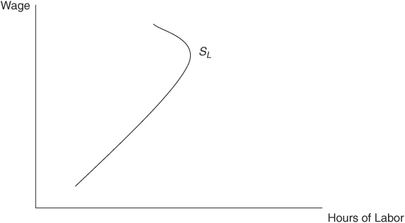
The two effects of a higher wage predict different impacts on the decision to supply hours of labor to the labor market. If the substitution effect is stronger than the income effect, the labor supply curve is upward-sloping; higher wages increase the hours of labor supplied. But at very high wages, the income effect might be stronger than the substitution effect, so that the supply of labor may be downward-sloping; higher wages decrease the hours of labor supplied. Figure 10-1 shows a labor supply (SL) curve that is “backward-bending” (downward-sloping) at high wages. Although this may indeed exist for some individuals, for most of us the labor supply curve is upward-sloping, and we will draw it as such throughout this chapter.
FIGURE 10.1 • Backward-Bending Labor Supply Curve
The other side of the labor market is, of course, labor demand. When deciding whether the next unit of labor should be hired, employers weigh the marginal benefits of hiring against the marginal costs of hiring. By now this decision-making process should sound familiar, but in this context we have slightly different names for the marginal benefits and costs. On the benefit side of the decision, employers are interested in two key variables: how much additional output the next unit of labor brings to the firm (the marginal product of labor, or MPL), and the market value of that output. For now, we assume that the firm sells its output in a perfectly competitive product market, so the market value of the output is simply the price (P). When we combine these two variables, we get the value of the marginal product of labor (VMPL):

Let’s use a quick example to show how this is computed. Suppose that Dora sells maps of historic sites to tourists that visit her city. The market for the maps is competitive, and the market price of a map is $5. Dora can employ workers, and the marginal productivity of each worker is shown in Table 10-1.
TABLE 10-1 Marginal Productivity of Labor
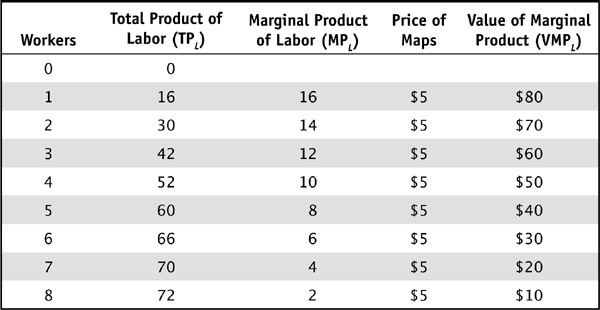
Like any profit-maximizing employer, Dora will not employ a worker if the marginal cost of employing that worker exceeds the value of the marginal product. Suppose the market wage is $40. At this wage, Dora will employ 5 workers to maximize her profit. Figure 10-2 shows this hiring decision as the intersection of the downward-sloping VMPL curve and the constant market wage. If the market wage rises to $50, Dora will reduce her hiring from 5 workers to 4. This inverse relationship between the wage and hiring is another example of the law of demand, and the VMPL curve serves as Dora’s demand for labor (DL) curve.
FIGURE 10-2 • Demand for Labor Curve
 Still Struggling?
How do we know that Dora’s employment of five workers at the wage of $40 is the profit-maximizing employment decision? Think of it marginally. If the marginal dollars of revenue earned from a hire at least exceed the marginal dollars of cost incurred from that hire, she should hire that worker because marginal profit is greater than or equal to zero. Table 10-2 shows this hiring decision again.
TABLE 10-2 Marginal Productivity of Labor and Profit
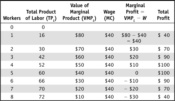
If we sum up all of the marginal profit gained from the first five workers, we get a total profit of $100. We can see from the table that employment of the sixth worker will actually cause profit to fall by $10.
In addition to wage-related movements along the labor demand curve, the labor demand curve can shift if one of several determinants of labor demand changes. We typically recognize four demand determinants in factor markets such as the market for labor.
1. The price of the output. If the price of the output increases, the VMPL will increase at all levels of employment, shifting the demand for labor to the right. The demand for a factor is described as a derived demand because it is derived from the demand for the goods that are being produced by the factor. For example, if the demand for steel increases, the price of steel increases, thus increasing the demand for steelworkers.
2. The price of substitute factors. All else equal, if the price of a substitute factor (like some forms of capital) increases, the firm’s demand for labor increases. This also works in reverse. If the price of industrial sewing machines decreases, the demand for textile workers decreases.
3. The price of complementary factors. All else equal, if the price of a complementary factor increases, the demand for labor decreases. If the price of diesel fuel increases, the demand for truck drivers decreases.
4. Productivity. If the marginal productivity of labor increases, the VMPL increases, and the demand for labor shifts to the right.
When factor markets are assumed to be competitive, wages are determined by the forces of supply and demand for that factor. In the example of Dora’s map-selling business, the market wage was $40, and Dora employed five workers. Suppose that there are 100 firms selling the maps in this competitive environment and that each firm is making the same hiring decision as Dora. We can then deduce that there are 500 workers employed in this labor market at the market wage of $40. Figure 10-4 shows equilibrium in the labor market.
FIGURE 10-4 • Labor Market Equilibrium
Equilibrium wages in factor markets are determined in the same way as equilibrium prices in output markets. If the demand for labor rises or the supply of labor falls, the wage rises. If the demand for labor falls or the supply of labor rises, the wage falls. For example, suppose that the population of the city declines, thus reducing the size of the labor force. As the supply of labor shifts to the left in Figure 10-5, employers like Dora find it more difficult to find people who are willing to work at the wage of $40. Because there is a shortage of workers at this wage, there is upward pressure on the wage. If the wage rises to $50, Dora will employ 4 workers and 400 will be employed in the entire market.
FIGURE 10-5 • A Shift to the Left of the Labor Supply Curve
In the long run, employers can adjust the hiring of all inputs. Suppose a firm can hire labor (L) at the market wage (w) and capital (K) at the market rate (r). For any level of output, the firm wishes to hire labor and capital to produce that output at the lowest possible cost. After all, if you could produce 100 maps at a cost of $500 or 100 maps at a cost of $1,000, you would be wise to avoid the second of these two situations. We have actually seen a similar problem in Chapter 2 when we studied how a consumer could choose quantities of two goods to produce as much utility as possible while being constrained by his budget line.
Suppose Dora can employ labor at the market wage of $40 and capital at the market rate of $10. If Dora needs to produce 100 maps each day, she has several different combinations of labor and capital from which to choose. Table 10-5 shows a few combinations and the total cost of employing each combination.
TABLE 10-5 Possible Combinations of Labor and Capital
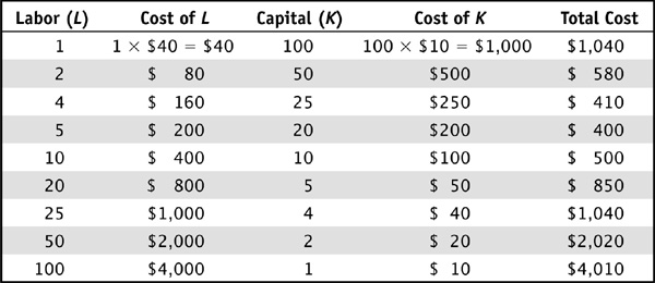
If she is limited to the choices in this table, clearly Dora should choose to employ 5 units of labor and 20 units of capital because the total cost of that combination is $400, the lowest in the table.
Let’s take a look at the hiring decision in a slightly different way and simplify the mathematics quite a bit. Suppose that both labor and capital can be hired at $1 per unit. In the current combination of labor and capital, Dora realizes that the marginal product of labor (MPL) is 50 units and the marginal product of capital (MPK) is 10 units. Should Dora maintain this hiring combination? No. If Dora hires one more unit of labor, output will rise by 50 units. To keep total costs the same, she must hire one less unit of capital, with the result that output will decline by 10 units. So this small adjustment increases output by 40 units and doesn’t increase total cost. What is happening here? The additional dollar spent on the next unit of labor was more productive than it would have been if she had spent it on capital, so it was best spent on labor.
Let’s compare the marginal product per dollar:

In Dora’s situation, she wisely increased labor and decreased capital, thus readjusting her hiring decision. When would Dora find that such a readjustment would not pay dividends? To answer this, we need to introduce something known as the least-cost hiring rule. To produce a given level of output at the lowest possible cost, inputs should be hired to the point where:

By rearranging the equation, we see an alternative way to think about the rule.

This looks very similar to the rule for maximizing utility in Chapter 2. In that situation, the consumer used his budget to buy goods X and Y to the point where the marginal utility per dollar was equal. The same logic is true here. When the additional output per dollar (the “bang for the buck”) is the same for both factors, there is no way to readjust the hiring to increase output at the same cost.
 Still Struggling?
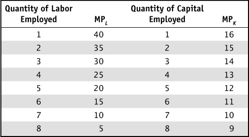
Let’s use an alternative example to see if we can find the least-cost combination of labor and capital. Suppose that your hiring budget cannot exceed $80, and so your goal is to produce as many units of output as possible for that budget. The price of labor is $20, and the price of capital is $10. The marginal products of labor and capital are given in Table 10-6.
TABLE 10-6 Marginal Products of Labor and Capital
Let’s begin with the least-cost hiring rule:

This tells us that we need to find combinations of labor and capital such that the marginal product of labor is twice the marginal product of capital. There are two possibilities in Table 10-6.
Combination A: 3 units of  and 2 units of
  . The total cost of this hiring combination is indeed $80 (3 labor at $20 each and 2 capital at $10 each = $80), and the output is 136 units (Total output
  .
.
Combination B: 5 units of  and 7 units of
  . The total cost of this hiring combination is $170, which is beyond our hiring budget.
There are other combinations of labor and capital that would spend exactly $80. For example, let’s consider one final combination.
Combination C: 2 units of labor  and 4 units of capital
  . While it’s true that this spends the $80 hiring budget, it’s also true that

If we left this hiring decision unchanged, total output would be only 133 units. But if we spent just a little more on labor and a little less on capital (Combination A) we could get 3 additional units of output and keep hiring costs the same.
When the wage rises, most people find that leisure becomes too costly, and they increase the hours of labor supplied to the labor market, thus giving us an upward-sloping labor supply curve. The downward-sloping labor demand curve comes from combining a downward-sloping marginal product of labor with the market price to compute the value of the marginal product. Because the profit-maximizing firm hires labor to the point where the market wage is equal to VMPL, this serves as the firm’s demand for labor. The competitive labor market determines the equilibrium wage and employment at the intersection of the demand and supply curves. Wages in this market rise and fall with the typical patterns of any competitive market. In the long run, when the firm can adjust both labor and capital, the firm seeks to find the least-cost combination of labor and capital to produce a given level of output. This occurs when the marginal product per dollar is equal for both factors.
This chapter concludes our coverage of what is typically seen as microeconomics. The next several chapters introduce and develop macroeconomics and show how all of the micro decisions affect the broader macro economy.
Is each of the following statements true or false? Explain.
1. There is no theoretical justification for a downward-sloping labor supply curve.
2. When markets are perfectly competitive, the VMPL curve is downward-sloping because of diminishing marginal returns to production.
3. If the VMPL curve shifts to the right, the firm will increase hiring to increase profits.
4. If the demand for labor increases and the supply of labor decreases, the wage will certainly rise.
5. The least-cost combination of labor and capital occurs when the marginal product of labor is equal to the marginal product of capital.
For each of the following, choose the answer that best fits.
6. When Eric’s wage falls, we predict that he will:
A. Decrease his hours of labor supplied because the substitution effect is greater than the income effect
B. Increase his hours of labor supplied because the substitution effect is greater than the income effect
C. Decrease his hours of labor supplied because the income effect is greater than the substitution effect
D. Increase his hours of labor supplied because there is no substitution effect when wages fall, there is only income effect
Use Table 10-7 to respond to questions 7 and 8.

7. This firm sells each unit of output in a perfectly competitive product market at a price of $10. The value of the marginal product of labor for the sixth worker is equal to:
A. $10
B. $14
C. $40
D. $16
8. If the competitive market wage is equal to $30 and the competitive price of the output is $3, how many workers will be employed to maximize profit?
A. 1
B. 2
C. 3
D. 4
9. The labor market for fast food workers is perfectly competitive and is currently in equilibrium. Suppose the cost of restaurant equipment (such as stoves, ovens, and dishwashers) falls. In the market for fast food workers, we predict that:
A. Wage rises and employment falls if the workers are substitutes.
B. Wage and employment both fall if the workers and equipment are substitutes.
C. Wage and employment both fall if the workers and equipment are complementary.
D. Wage falls and employment rises if the workers and equipment are complementary.
10. Stanley is currently employing labor at a wage of $5 per unit, and capital at a rate of $25 per unit. The marginal product of labor is currently equal to 20 units, and the marginal product of capital is equal to 100 units. Stanley should:
A. Increase hiring of both labor and capital.
B. Increase hiring of labor and decrease hiring of capital.
C. Decrease hiring of labor and increase hiring of capital.
D. Do nothing; he has already hired the least-cost combination of labor and capital.