When given measures μ
1, …, μ
N are supported on the real line, computing their Fréchet mean  is straightforward (Sect. 3.1.4). This is in contrast to the multivariate case, where, apart from the important yet special case of compatible measures, closed-form formulae are not available. This chapter presents an iterative procedure that provably approximates at least a Karcher mean with mild restrictions on the measures μ
1, …, μ
N. The algorithm is based on the differentiability properties of the Fréchet functional developed in Sect. 3.1.6 and can be interpreted as classical steepest descent in the Wasserstein space
  . It reduces the problem of finding the Fréchet mean to a succession of pairwise transport problems, involving only the Monge–Kantorovich problem between two measures. In the Gaussian case (or any location-scatter family), the latter can be done explicitly, rendering the algorithm particularly appealing (see Sect. 5.4.1).
This chapter can be seen as a complementary to Chap. 4. On the one hand, one can use the proposed algorithm to construct the regularised Fréchet–Wasserstein estimator  that approximates a population version (see Sect. 4.3). On the other hand, it could be that the object of interest is the sample μ
1, …, μ
N itself, but that the latter is observed with some amount of noise. If one only has access to proxies
  , then it is natural to use their Fréchet mean
  as an estimator of
  . The proposed algorithm can then be used, in principle, in order to construct
  , and the consistency framework of Sect. 4.4 then allows to conclude that if each
  is consistent, then so is
  .
.
After presenting the algorithm in Sect. 5.1, we make some connections to Procrustes analysis in Sect. 5.2. A convergence analysis of the algorithm is carried out in Sect. 5.3, after which examples are given in Sect. 5.4. An extension to infinitely many measures is sketched in Sect. 5.5.
5.1 A Steepest Descent Algorithm for the Computation of Fréchet Means

 is sought. It has been established that if γ is absolutely continuous then the associated Fréchet functional

 be an absolutely continuous measure, representing our current estimate of the Fréchet mean at step j. Then it makes sense to introduce a step size τ
j > 0, and to follow the steepest descent of F given by the negative of the gradient:
 ![$$\displaystyle \begin{aligned} \gamma_{j+1} =\exp_{\gamma_j} \left(-\tau_j F'(\gamma_j)\right) = \left[{\mathbf i} + \tau_j\frac 1N \sum_{i=1}^N \log_{\gamma}(\mu^i)\right]\#\gamma_j =\left[{\mathbf i} + \tau_j\frac 1N\sum_{i=1}^N ({\mathbf{t}}_{\gamma_j}^{\mu^i} - {\mathbf i})\right]\#\gamma_j. \end{aligned}$$](../images/456556_1_En_5_Chapter/456556_1_En_5_Chapter_TeX_Equb.png)
If γ
0 is absolutely continuous and τ = τ
0 ∈ [0, 1], then  is also absolutely continuous.
The idea is that push-forwards of γ 0 under monotone maps are absolutely continuous if and only if the monotonicity is strict, a property preserved by averaging. See page 118 in the supplement for the details.
Lemma 5.1.1 suggests that the step size should be restricted to [0, 1]. The next result suggests that the objective function essentially tells us that the optimal step size, achieving the maximal reduction of the objective function (thus corresponding to an approximate line search), is exactly equal to 1. It does not rely on finite-dimensional arguments and holds when replacing  by a separable Hilbert space.
 is absolutely continuous, then
![$$\displaystyle \begin{aligned} F(\gamma_{1})-F(\gamma_0) \le - \|F'(\gamma_0)\|{}^2\left[\tau - \frac{\tau^2}2 \right] \end{aligned}$$](../images/456556_1_En_5_Chapter/456556_1_En_5_Chapter_TeX_Equc.png)
and the bound on the right-hand side of the last display is minimised when τ = 1.
 be the optimal map from γ
0 to μ
i, and set W
i = S
i −i. Then
![$$\displaystyle \begin{aligned} W_2^2(\gamma_1,\mu^i) \le \int_{{\mathbb R^d}}{\left\|\left[(1-\tau)\mathbf i+\frac\tau N\sum_{j=1}^NS_j\right] - S_i\right\|{}_{\mathbb R^d}^2}\mathrm{d}{\gamma_0} = \left\| -W_i + \frac \tau N\sum_{j=1}^NW_j\right\|{}^2_{\mathcal L^2(\gamma_0)}. \end{aligned}$$](../images/456556_1_En_5_Chapter/456556_1_En_5_Chapter_TeX_Equd.png)
 from the norms and inner products. Developing the squares, summing over i = 1, …, N and using (5.3) gives
![$$\displaystyle \begin{aligned} F(\gamma_1) - F(\gamma_0) \le \frac{\tau^2 - 2\tau}2\left\|\frac 1N\sum_{i=1}^NW_i\right\|{}^2 = -\|F'(\gamma_0)\|{}^2\left[\tau - \frac{\tau^2}2\right]. \end{aligned}$$](../images/456556_1_En_5_Chapter/456556_1_En_5_Chapter_TeX_Equf.png)

The proof of Proposition
3.1.2
suggests a generalisation of Algorithm
1to arbitrary measures in
 even if none are absolutely continuous. One can verify that Lemmata
5.1.2and
5.3.5(below) also hold in this setup, so it may be that convergence results also apply in this setup. The iteration no longer has the interpretation as steepest descent, however.
- (A)
Set a tolerance threshold 𝜖 > 0.
- (B)
For j = 0, let γ j be an arbitrary absolutely continuous measure.
- (C)
For i = 1, …, N solve the (pairwise) Monge problem and find the optimal transport map
 from γ
j to μ
i.
 - (D)
Define the map
 .
. - (E)
Set γ j+1 = T j#γ j, i.e. push-forward γ j via T j to obtain γ j+1.
- (F)
If ∥F′(γ j+1)∥ < 𝜖, stop, and output γ j+1 as the approximation of
 and
and  as the approximation of
  , i = 1, …, N. Otherwise, return to step (C).
5.2 Analogy with Procrustes Analysis
Algorithm 1 is similar in spirit to another procedure, generalised Procrustes analysis, that is used in shape theory. Given a subset  , most commonly a finite collection of labelled points called landmarks, an interesting question is how to mathematically define the shape of B. One way to reach such a definition is to disregard those properties of B that are deemed irrelevant for what one considers this shape should be; typically, these would include its location, its orientation, and/or its scale. Accordingly, the shape of B can be defined as the equivalence class consisting of all sets obtained as gB, where g belongs to a collection
  of transformations of
  containing all combinations of rotations, translations, dilations, and/or reflections (Dryden and Mardia [45, Chapter 4]).
If B
1 and B
2 are two collections of k landmarks, one may define the distance between their shapes as the infimum of ∥B
1 − gB
2∥2 over the group  . In other words, one seeks to register B
2 as close as possible to B
1 by using elements of the group
  , with distance being measured as the sum of squared Euclidean distances between the transformed points of B
2 and those of B
1. In a sense, one can think about the shape problem and the Monge problem as dual to each other. In the former, one is given constraints on how to optimally carry out the registration of the points with the cost being judged by how successful the registration procedure is. In the latter, one imposes that the registration be done exactly, and evaluates the cost by how much the space must be deformed in order to achieve this.
The optimal g and the resulting distance can be found in closed-form by means of ordinary Procrustes analysis [45, Section 5.2]. Suppose now that we are given N > 2 collections of points, B
1, …, B
N, with the goal of minimising the sum of squares ∥g
iB
i − g
jB
j∥2 over  .1 As in the case of Fréchet means in
  (Sect. 3.1.2), there is a formulation in terms of sum of squares from the average
  . Unfortunately, there is no explicit solution for this problem when d ≥ 3. Like Algorithm 1, generalised Procrustes analysis (Gower [66]; Dryden and Mardia [45, p. 90]) tackles this “multimatching” setting by iteratively solving the pairwise problem as follows. Choose one of the configurations as an initial estimate/template, then register every other configuration to the template, employing ordinary Procrustes analysis. The new template is then given by the linear average of the registered configurations, and the process is iterated subsequently.
- (1)
Registration: by finding the optimal transportation maps
 , we identify each μ
i with the element
  . In this sense, the collection (μ
1, …, μ
N) is viewed in the common coordinate system given by the tangent space at the template γ
j and is registered to it.
 - (2)
Averaging: the registered measures are averaged linearly, using the common coordinate system of the registration step (1), as elements in the linear space
 . The linear average is then retracted back onto the Wasserstein space via the exponential map to yield the estimate at the (j + 1)-th step, γ
j+1.
 , the inverses of
  . We will not use the term “registration maps” in the sequel, to avoid possible confusion.
5.3 Convergence of Algorithm 1
In order to tackle the issue of convergence, we will use an approach that is specific to the nature of optimal transport. This is because the Hessian-type arguments that are used to prove similar convergence results for steepest descent on Riemannian manifolds (Afsari et al. [1]) or Procrustes algorithms (Le [86]; Groisser [67]) do not apply here, since the Fréchet functional may very well fail to be twice differentiable.
In fact, even in Euclidean spaces, convergence of steepest descent usually requires a Lipschitz bound on the derivative of F (Bertsekas [19, Subsection 1.2.2]). Unfortunately, F is not known to be differentiable at discrete measures, and these constitute a dense set in  ; consequently, this Lipschitz condition is very unlikely to hold. Still, this specific geometry of the Wasserstein space affords some advantages; for instance, we will place no restriction on the starting point for the iteration, except that it be absolutely continuous; and no assumption on how “spread out” the collection μ
1, …, μ
N is will be necessary as in, for example, [1, 67, 86].
Let  be probability measures and suppose that one of them is absolutely continuous with a bounded density. Then, the sequence generated by Algorithm 1 stays in a compact set of the Wasserstein space
  , and any limit point of the sequence is a Karcher mean of (μ
1, …, μ
N).
Since the Fréchet mean  is a Karcher mean (Proposition 3.1.8), we obtain immediately:
Alternatively, combining Theorem 5.3.1 with the optimality criterion Theorem 3.1.15 shows that the algorithm converges to  when the appropriate assumptions on {μ
i} and the Karcher mean
  are satisfied. This allows to conclude that Algorithm 1 converges to the unique Fréchet mean when μ
i are Gaussian measures (see Theorem 5.4.1).
The proof of Theorem 5.3.1 is rather elaborate, since we need to use specific methods that are tailored to the Wasserstein space. Before giving the proof, we state two important consequences. The first is the uniform convergence of the optimal maps  to
to  on compacta. This convergence does not immediately follow from the Wasserstein convergence of γ
j to
  , and is also established for the inverses. Both the formulation and the proof of this result are similar to those of Theorem 4.4.3.
for any pair of compacta Ω
1 ⊆ A,  . If in addition all the measures μ
1, …, μ
N have the same support, then one can choose all the sets B
i to be the same.
The other consequence is convergence of the optimal multicouplings.

of {μ
1, …, μ
N} converges (in Wasserstein distance on  ) to the optimal multicoupling
  .
.
The proofs of Theorem 5.3.3 and Corollary 5.3.4 are given at the end of the present section.
The sequence generated by Algorithm 1 stays in a compact subset of the Wasserstein space  .
.
For all j ≥ 1, γ
j takes the form M
n#π, where  and π is a multicoupling of μ
1, …, μ
N. The compactness of this set has been established in Step 2 of the proof of Theorem 3.1.5; see page 63 in the supplement, where this is done in a more complicated setup.
A closer look at the proof reveals that a more general result holds true. Let  denote the steepest descent iteration, that is,
  . Then the image of
  ,
,  absolutely continuous} has a compact closure in
  . This is also true if
  is replaced by a separable Hilbert space.
In order to show that a weakly convergent sequence (γ
j) of absolutely continuous measures has an absolutely continuous limit γ, it suffices to show that the densities of γ
j are uniformly bounded. Indeed, if C is such a bound, then for any open  ,
,  , so γ(O) ≤ CLeb(O) by the portmanteau Lemma 1.7.1. It follows that γ is absolutely continuous with density bounded by C. We now show that such C can be found that applies to all measures in the image of
  , hence to all sequences resulting from iterations of Algorithm 1.
 is bounded by the 1∕d-th harmonic mean of ∥g
i∥∞,
 ![$$\displaystyle \begin{aligned} C_{\mu} =\left[ \frac 1N \sum_{i=1}^N \frac 1{\|g^i\|{}_\infty^{1/d}} \right]^{-d}. \end{aligned}$$](../images/456556_1_En_5_Chapter/456556_1_En_5_Chapter_TeX_Equk.png)
The constant C μ depends only on the measures (μ 1, …, μ N), and is finite as long as one μ i has a bounded density, since C μ ≤ N d∥g i∥∞ for any i.

 , which by definition equals
![$$\displaystyle \begin{aligned}{}[\det(A+B)]^{1/d} \ge [\det A]^{1/d} + [\det B]^{1/d}, \end{aligned}$$](../images/456556_1_En_5_Chapter/456556_1_En_5_Chapter_TeX_Equn.png)
![$$\displaystyle \begin{aligned} \left[\det\nabla {\mathbf{t}}_{\gamma_0}^{\gamma_1}(x)\right]^{1/d} \ge \frac 1N \sum_{i=1}^N \left[\det\nabla {\mathbf{t}}_{\gamma_0}^{\mu^i}(x)\right]^{1/d} . \end{aligned}$$](../images/456556_1_En_5_Chapter/456556_1_En_5_Chapter_TeX_Equo.png)
![$$\displaystyle \begin{aligned} \frac 1{h_1^{1/d}({\mathbf{t}}_{\gamma_0}^{\gamma_1}(x))} {=}\frac {\det^{1/d}\sum_{i=1}^N \nabla {\mathbf{t}}_{\gamma_0}^{\mu^i}(x)}{N h_0^{1/d}(x)} {\ge} \frac 1N \sum_{i=1}^N \frac {1}{[g^i({\mathbf{t}}_{\gamma_0}^{\mu^i}(x))]^{1/d}} {\ge} \frac 1N \sum_{i=1}^N \frac 1{\|g^i\|{}_\infty^{1/d}} =C_\mu^{-1/d}. \end{aligned}$$](../images/456556_1_En_5_Chapter/456556_1_En_5_Chapter_TeX_Equp.png)
![$$\displaystyle \begin{aligned} \gamma_1({\mathbf{t}}_{\gamma_0}^{\gamma_1}(\varSigma)) = \gamma_0[({\mathbf{t}}_{\gamma_0}^{\gamma_1})^{-1}({\mathbf{t}}_{\gamma_0}^{\gamma_1}(\varSigma))] \ge \gamma_0(\varSigma)=1. \end{aligned}$$](../images/456556_1_En_5_Chapter/456556_1_En_5_Chapter_TeX_Equq.png)

The third statement (continuity of  ) is much more subtle to establish, and its rather lengthy proof is given next. In view of Proposition 5.3.6, the uniform bound on the densities is not a hindrance for the proof of convergence of Algorithm 1.

Then η
j → η in ![$${\mathcal {W}}_2([{\mathbb {R}}^d]^{N+1})$$](../images/456556_1_En_5_Chapter/456556_1_En_5_Chapter_TeX_IEq67.png) .
.
As has been established in the discussion before Proposition 5.3.6, the limit γ must be absolutely continuous, so η is well-defined.
 is any continuous nonnegative function such that

 is uniformly close to g
n:
 ![$$\displaystyle \begin{aligned} \sup_n \int {[g_n(x) - g_{n,R}(x)]}\mathrm{d}{\gamma_n(x)} \to0, \qquad R\to\infty. \end{aligned}$$](../images/456556_1_En_5_Chapter/456556_1_En_5_Chapter_TeX_Equv.png)
 converge to
  and (since h is continuous), g
n → g uniformly on “nice” sets Ω ⊆ E = suppγ. Write
Step 3: Bounding the first two integrals. The first integral vanishes as n →∞, by the portmanteau Lemma 1.7.1, and the second by uniform convergence.
Step 4: Bounding the third integral. The integrand is bounded by 8R, so it suffices to bound the measures of  . This is a bit technical, and uses the uniform density bound on (γ
n) and the portmanteau lemma.
 )
)If W
2(γ
n, γ) → 0 and γ
n have uniformly bounded densities, then  .
.
Choose h in the proof of Proposition 5.3.7 to depend only on y.
Choose h in the proof of Proposition 5.3.7 to depend only on t 1, …, t n.
Let  and set
  univalued}. As
  is absolutely continuous,
  , and the same is true for
  . The first assertion then follows from Proposition 1.7.11.
The second statement is proven similarly. Let E
i = suppμ
i and notice that by absolute continuity the  has measure 1 with respect to μ
i. Apply Proposition 1.7.11. If in addition E
1 = ⋯ = E
N, then μ
i(B) = 1 for B = ∩B
i.
5.4 Illustrative Examples
As an illustration, we implement Algorithm 1 in several scenarios for which pairwise optimal maps can be calculated explicitly at every iteration, allowing for fast computation without error propagation. In each case, we give some theory first, describing how the optimal maps are calculated, and then implement Algorithm 1 on simulated examples.
5.4.1 Gaussian Measures
![$$\displaystyle \begin{aligned} {\mathbf{t}}_{A}^{B}(x) = A^{-1/2} [A^{1/2}BA^{1/2}]^{1/2} A^{-1/2}x, \qquad x\in {\mathbb{R}}^d, \end{aligned}$$](../images/456556_1_En_5_Chapter/456556_1_En_5_Chapter_TeX_Equx.png)
![$$\displaystyle \begin{aligned} \varGamma =\frac 1N\sum_{i=1}^N \left[\varGamma^{1/2}S_i\varGamma^{1/2}\right]^{1/2}, \end{aligned} $$](../images/456556_1_En_5_Chapter/456556_1_En_5_Chapter_TeX_Equ4.png)
Given the formula for  , application of Algorithm 1 to Gaussian measures is straightforward. The next result shows that, in the Gaussian case, the iterates must converge to the unique Fréchet mean, and that (5.4) can be derived from the characterisation of Karcher means.
Let μ
1, …, μ
N be Gaussian measures with zero means and covariance matrices S
i with S
1 nonsingular, and let the initial point γ
0 be  with Γ
0 nonsingular. Then the sequence of iterates generated by Algorithm 1 converges to the unique Fréchet mean of (μ
1, …, μ
N).
Since the optimal maps are linear, so is their mean and therefore γ
k is a Gaussian measure for all k, say  with Γ
k nonsingular. Any limit point of γ is a Karcher mean by Theorem 5.3.1. If we knew that γ itself were Gaussian, then it actually must be the Fréchet mean because
  equals the identity everywhere on
  (see the discussion before Theorem 3.1.15).
Let us show that every limit point γ is indeed Gaussian. It suffices to prove that (Γ
k) is a bounded sequence, because if Γ
k → Γ, then  weakly, as can be seen from either Lehmann–Scheffé’s theorem (the densities converge) or Lévy’s continuity theorem (the characteristic functions converge).
![$$\displaystyle \begin{aligned} W^2_2(\mu,\delta_0) ={{\mathrm{tr}}} [S], \end{aligned}$$](../images/456556_1_En_5_Chapter/456556_1_En_5_Chapter_TeX_Equy.png)
![$$\displaystyle \begin{aligned} 0\le {{\mathrm{tr}}}[\varGamma_k] =W_2^2(\gamma_k,\delta_0) \end{aligned}$$](../images/456556_1_En_5_Chapter/456556_1_En_5_Chapter_TeX_Equz.png)
![$$\displaystyle \begin{aligned} I =\frac 1N\sum_{i=1}^N \varGamma^{-1/2} \left[\varGamma^{1/2}S_i\varGamma^{1/2}\right]^{1/2} \varGamma^{-1/2} \end{aligned}$$](../images/456556_1_En_5_Chapter/456556_1_En_5_Chapter_TeX_Equaa.png)
If the means are nonzero, then the optimal maps are affine and the same result applies; the Fréchet mean is still a Gaussian measure with covariance matrix Γ and mean that equals the average of the means of μ i, i = 1, …, N.
 with covariances S
i ∼Wishart(I
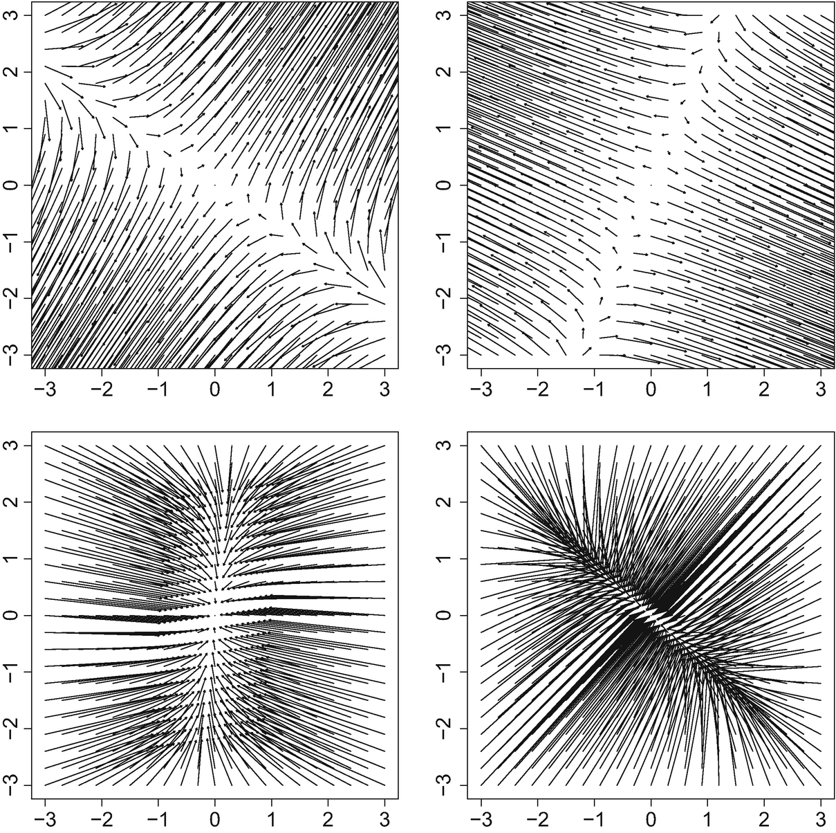
2, 2), and Fig. 5.2 shows the density of the resulting Fréchet mean. In this particular example, the algorithm needed 11 iterations starting from the identity matrix. The corresponding optimal maps are displayed in Fig. 5.3. It is apparent from the figure that these maps are linear, and after a more careful reflection one can be convinced that their average is the identity. The four plots in the figure are remarkably different, in accordance with the measures themselves having widely varying condition numbers and orientations; μ
3 and more so μ
4 are very concentrated, so the optimal maps “sweep” the mass towards zero. In contrast, the optimal maps to μ
1 and μ
2 spread the mass out away from the origin.
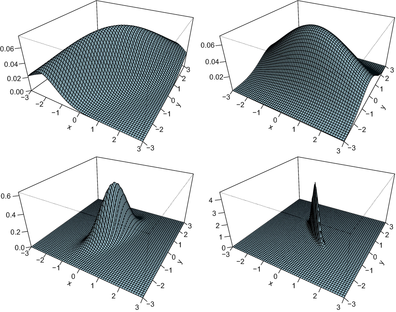
Density plot of four Gaussian measures in  .
.
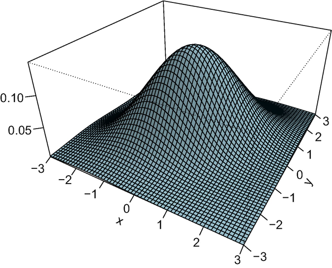
Density plot of the Fréchet mean of the measures in Fig. 5.1
5.4.2 Compatible Measures
We next discuss the behaviour of the algorithm when the measures are compatible. Recall that a collection  is compatible if for all
  ,
,  in L
2(γ) (Definition 2.3.1). Boissard et al. [28] showed that when this condition holds, the Fréchet mean of (μ
1, …, μ
N) can be found by simple computations involving the iterated barycentre. We again denote by γ
0 the initial point of Algorithm 1, which can be any absolutely continuous measure.
If γ 0 ∪{μ i} is compatible, then Algorithm 1 converges to the Fréchet mean of (μ i) after a single step.
![$$\displaystyle \begin{aligned} \gamma_1 =\left[\frac 1N\sum_{i=1}^N \mathbf t_{\gamma_0}^{\mu^i} \right]\#\gamma_0 , \end{aligned}$$](../images/456556_1_En_5_Chapter/456556_1_En_5_Chapter_TeX_Equab.png)
In this case, Algorithm 1 requires the calculation of N pairwise optimal maps, and this can be reduced to N − 1 if the initial point is chosen to be μ 1. This is the same computational complexity as the calculation of the iterated barycentre proposed in [28].
When the measures have a common copula, finding the optimal maps reduces to finding the optimal maps between the one-dimensional marginals (see Lemma 2.3.3) and this can be done using quantile functions as described in Sect. 1.5. The marginal Fréchet means are then plugged into the common copula to yield the joint Fréchet mean. We next illustrate Algorithm 1 in three such scenarios.
5.4.2.1 The One-Dimensional Case
 , we may apply Algorithm 1 starting from one of these measures (or any other measure). Figure 5.4 plots N = 4 univariate densities and the Fréchet mean yielded by the algorithm in two different scenarios. At the left, the densities were generated as
![$$\displaystyle \begin{aligned} m^i_1\sim U[-13, -3],\quad m^i_2\sim U[3, 13],\quad \sigma^i_1,\sigma^i_2\sim Gamma(4, 4). \end{aligned}$$](../images/456556_1_En_5_Chapter/456556_1_En_5_Chapter_TeX_Equac.png)

![$$\displaystyle \begin{aligned} \beta^i\sim Gamma(4, 1) ,\quad m^i_3\sim U[1,4] ,\quad m^i_4\sim U[-4,-1]. \end{aligned}$$](../images/456556_1_En_5_Chapter/456556_1_En_5_Chapter_TeX_Equad.png)
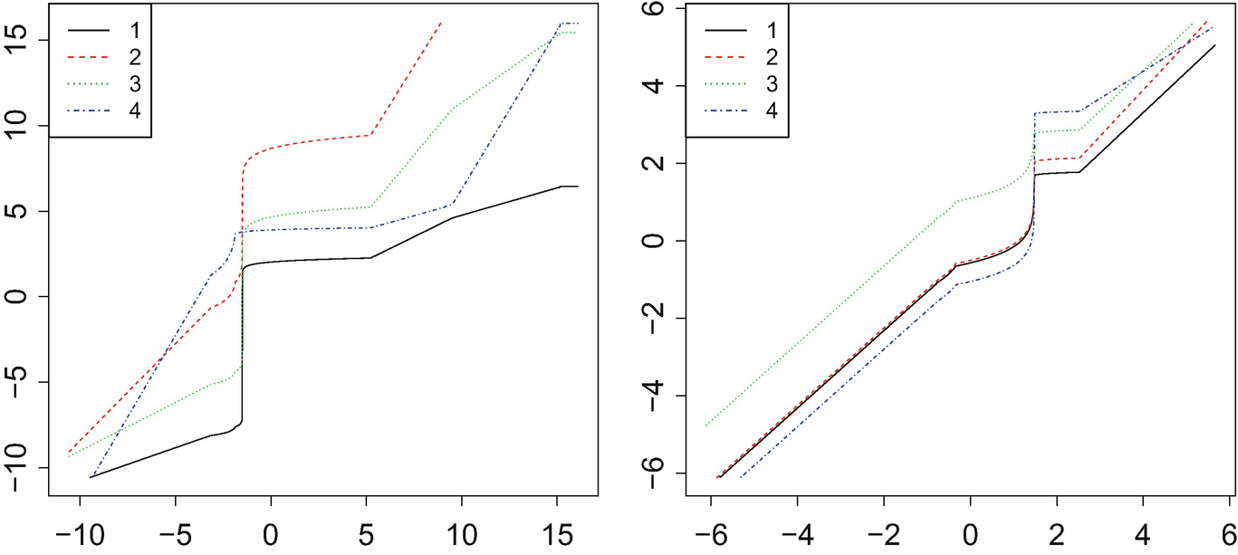
 to the measures μ
1, …, μ
N in each case. If one ignores the “middle part” of the x axis, the maps appear (approximately) affine for small values of x and for large values of x, indicating how the peaks are shifted. In the middle region, the maps need to “bridge the gap” between the different slopes and intercepts of these affine maps.
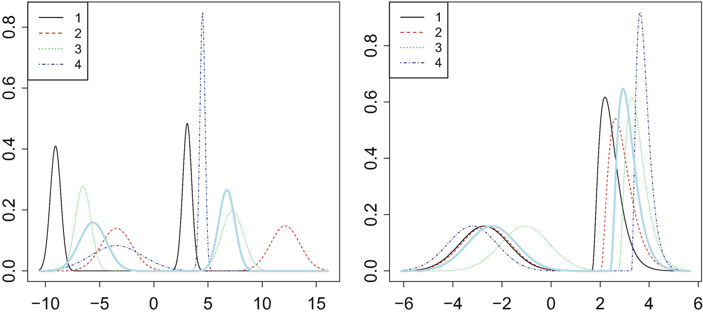
Densities of a bimodal Gaussian mixture (left) and a mixture of a Gaussian with a gamma (right), with the Fréchet mean density in light blue
Optimal maps  from the Fréchet mean
  to the four measures {μ
i} in Fig. 5.4. The left plot corresponds to the bimodal Gaussian mixture, and the right plot to the Gaussian/gamma mixture
5.4.2.2 Independence
 , having independent marginal densities
  as in (5.5), and
  as in (5.6). Figure 5.6 shows the density plot of N = 4 such measures, constructed as the product of the measures from Fig. 5.4. One can distinguish the independence by the “parallel” structure of the figures: for every pair (y
1, y
2), the ratio g(x, y
1)∕g(x, y
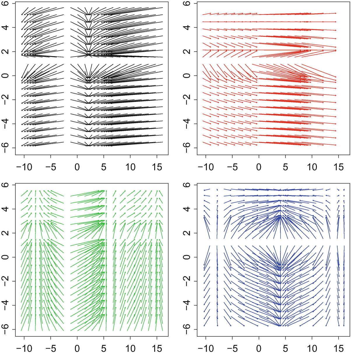
2) does not depend on x (and vice versa, interchanging x and y). Figure 5.7 plots the density of the resulting Fréchet mean. We observe that the Fréchet mean captures the four peaks and their location. Furthermore, the parallel nature of the figure is preserved in the Fréchet mean. Indeed, by Lemma 3.1.11 the Fréchet mean is a product measure. The optimal maps, in Fig. 5.10, are the same as in the next example, and will be discussed there.
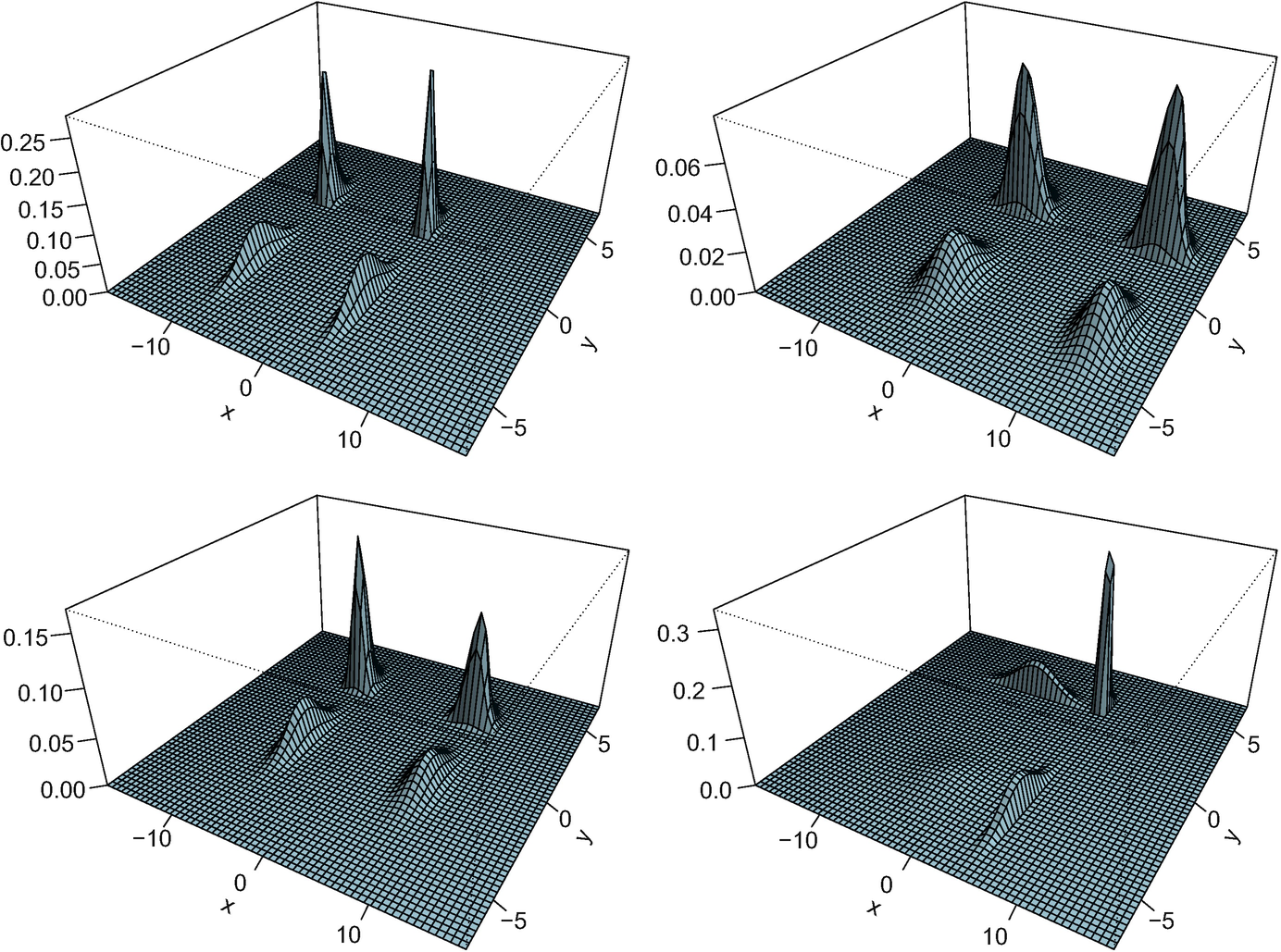
Density plots of the four product measures of the measures in Fig. 5.4
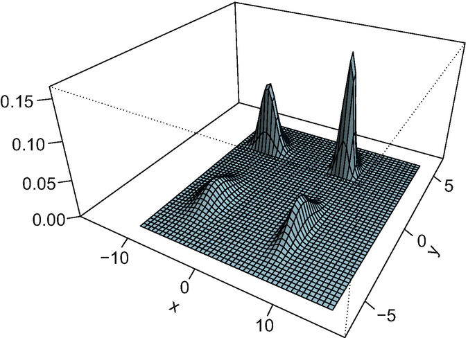
Density plot of the Fréchet mean of the measures in Fig. 5.6
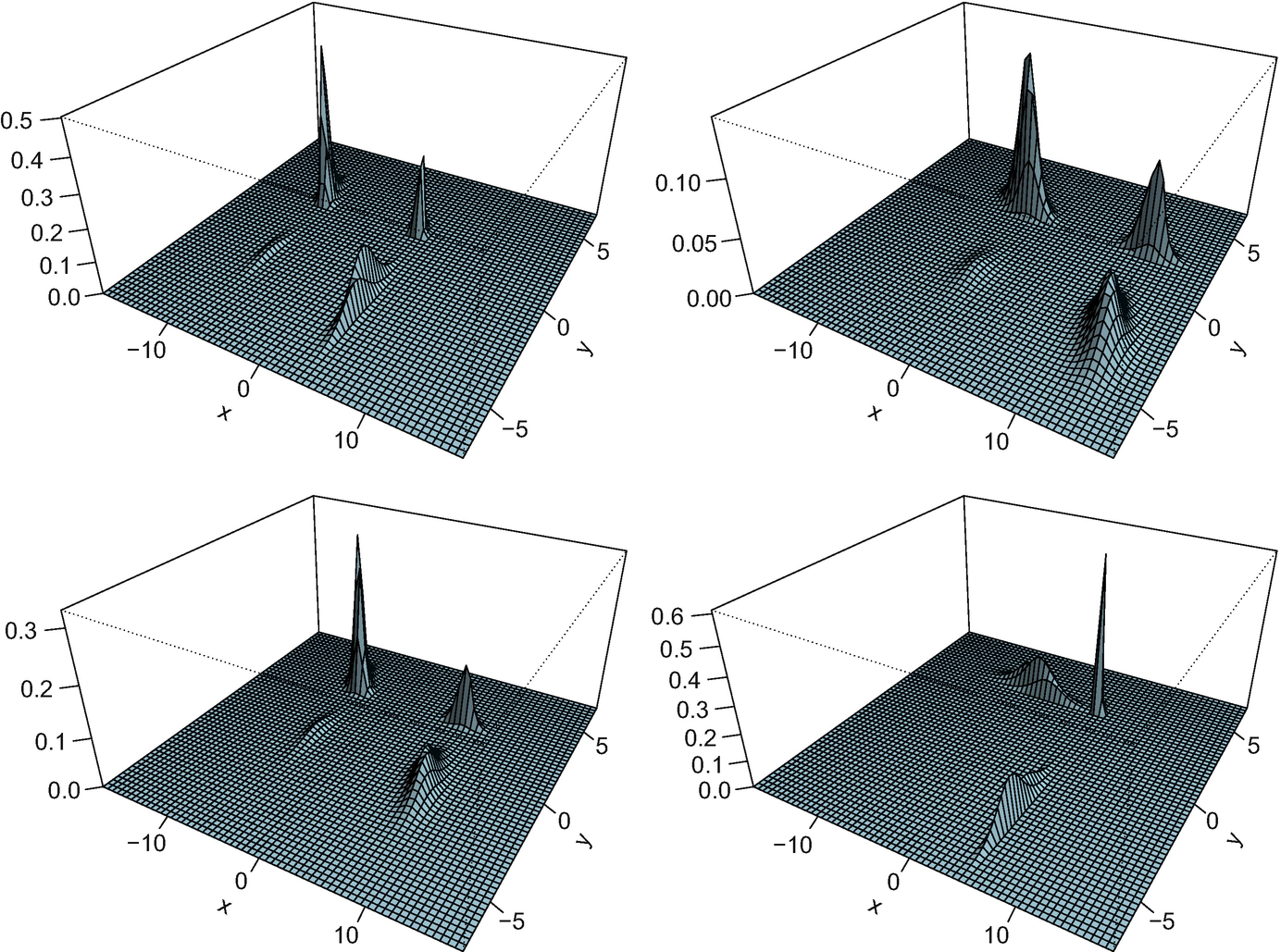
Density plots of four measures in  with Frank copula of parameter − 8
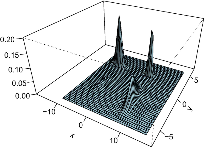
Density plot of the Fréchet mean of the measures in Fig. 5.8
5.4.2.3 Common Copula
 with density
 and
and  are random densities on the real line with distribution functions
  and
and  , and c is a copula density. Figure 5.8 shows the density plot of N = 4 such measures, with
  generated as in (5.5),
  as in (5.6), and c is the Frank(− 8) copula density, while Fig. 5.9 plots the density of the Fréchet mean obtained. (For ease of comparison we use the same realisations of the densities that appear in Fig. 5.4.) The Fréchet mean can be seen to preserve the shape of the density, having four clearly distinguished peaks. Figure 5.10, depicting the resulting optimal maps, allows for a clearer interpretation: for instance, the leftmost plot (in black) shows more clearly that the map splits the mass around x = −2 to a much wider interval; and conversely a very large amount mass is sent to x ≈ 2. This rather extreme behaviour matches the peak of the density of μ
1 located at x = 2.
as in (5.6), and c is the Frank(− 8) copula density, while Fig. 5.9 plots the density of the Fréchet mean obtained. (For ease of comparison we use the same realisations of the densities that appear in Fig. 5.4.) The Fréchet mean can be seen to preserve the shape of the density, having four clearly distinguished peaks. Figure 5.10, depicting the resulting optimal maps, allows for a clearer interpretation: for instance, the leftmost plot (in black) shows more clearly that the map splits the mass around x = −2 to a much wider interval; and conversely a very large amount mass is sent to x ≈ 2. This rather extreme behaviour matches the peak of the density of μ
1 located at x = 2.5.4.3 Partially Gaussian Trivariate Measures
![$$\displaystyle \begin{aligned} g^i(y_1,y_2,y_3) =g^i(y) =f^i(U_3^ty) \frac 1{2\pi\sqrt{\det S^i}} \exp\left[-\frac{(U_1^ty, U_2^ty)(S^i)^{-1}\binom{U_1^ty}{U_2^ty}}2\right],\end{aligned} $$](../images/456556_1_En_5_Chapter/456556_1_En_5_Chapter_TeX_Equaf.png)
 positive definite. We simulated N = 4 such densities with f
i as in (5.5) and S
i ∼Wishart(I
2, 2). We apply Algorithm 1 to this collection of measures and find their Fréchet mean (see the end of this subsection for precise details on how the optimal maps were calculated). Figure 5.11 shows level set of the resulting densities for some specific values. The bimodal nature of f
i implies that for most values of a, {x : f
i(x) = a} has four elements. Hence, the level sets in the figures are unions of four separate parts, with each peak of f
i contributing two parts that form together the boundary of an ellipsoid in
  (see Fig. 5.12). The principal axes of these ellipsoids and their position in
  differ between the measures, but the Fréchet mean can be viewed as an average of those in some sense.
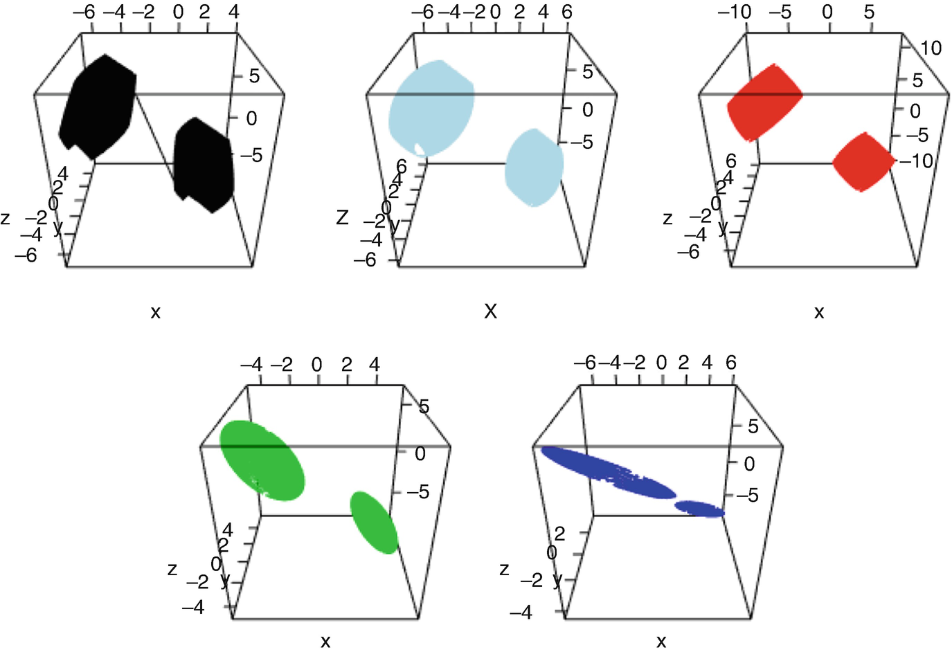
The set  for i = 1 (black), the Fréchet mean (light blue), i = 2, 3, 4 in red, green, and dark blue, respectively
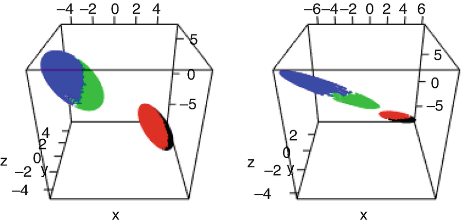
The set  for i = 3 (left) and i = 4 (right), with each of the four different inverses of the bimodal density f
i corresponding to a colour
In terms of orientation (principal axes) of the ellipsoids, the Fréchet mean is most similar to μ 1 and μ 2, whose orientations are similar to one another.
![$$\displaystyle \begin{aligned} f^i(x_3)\exp\left[-\frac{(x_1,x_2)(\varSigma^i)^{-1}\binom{x_1}{x_2}}2\right] \frac 1{2\pi\sqrt{\det \varSigma^i}}, \end{aligned}$$](../images/456556_1_En_5_Chapter/456556_1_En_5_Chapter_TeX_Equag.png)
 . By Lemma 3.1.11, the Fréchet mean of (U
−1#μ
i) is the product measure of that of (ρ
i) and that of (ν
i); by Lemma 3.1.12, the Fréchet mean of (μ
i) is therefore
 , with ν
0 having continuous distribution
  , the optimal maps are
  with
with 

 with the positive definite matrix (Σ
i)1∕2[(Σ
i)1∕2Σ
0(Σ
i)1∕2]−1∕2 (Σ
i)1∕2 that pushes forward
  to
to  . Due to the one-dimensionality, the algorithm finds the third component of the rotated measures after one step, but the convergence of the Gaussian component requires further iterations.
5.5 Population Version of Algorithm 1
 be a random measure with finite Fréchet functional. The population version of (5.1) is


 .
.
 because the random map
  is measurable (Lemma 2.4.6). Since
  is a Hilbert space, the law of large numbers applies there, and results for the empirical version carry over to the population version by means of approximations. In particular:
Any descent iterate γ has density bounded by q −dM, where q and M are as in (5.7).
The result is true in the empirical case, by Proposition 5.3.6. The key point (observed by Pass [102, Subsection 3.3]) is that the number of measures does not appear in the bound q −dM.
 and q
n → q almost surely by the law of large numbers. Pick any ω in the probability space for which this happens and notice that (invoking Lemma 2.4.5)
 ![$$\displaystyle \begin{aligned} \mathcal A(\gamma) =\left[\lim_{n\to\infty} \frac 1n\sum_{i=1}^n {\mathbf{t}}_{\gamma}^{\varLambda_i}\right] \# \gamma =\lim_{n\to\infty} \left[\frac 1n\sum_{i=1}^n {\mathbf{t}}_{\gamma}^{\varLambda_i}\right] \# \gamma. \end{aligned}$$](../images/456556_1_En_5_Chapter/456556_1_En_5_Chapter_TeX_Equan.png)
 almost surely, so for any C > q
−dM and n large, λ
n has density bounded by C. By the portmanteau Lemma 1.7.1, so does
 ![$$\lim \lambda _n=[{\mathbb {E}} {\mathbf {t}}_{\gamma }^{\varLambda }]\#\gamma $$](../images/456556_1_En_5_Chapter/456556_1_En_5_Chapter_TeX_IEq130.png) . Now let
. Now let  .
.Though it follows that every Karcher mean of Λ has a bounded density, we cannot yet conclude that the same bound holds for the Fréchet mean, because we need an a-priori knowledge that the latter is absolutely continuous. This again can be achieved by approximations:
Let
 be a random measure with finite Fréchet functional. If Λ has a bounded density with positive probability, then the Fréchet mean of Λ is absolutely continuous with a bounded density.
Let q and M be as in (5.7), Λ
1, … be a sample from Λ, and q
n the proportion of (Λ
i)i≤n with density bounded by M. The empirical Fréchet mean λ
n of the sample (Λ
1, …, Λ
n) has a density bounded by  . The Fréchet mean λ of Λ is unique by Proposition 3.2.7, and consequently λ
n → λ in
  by the law of large numbers (Corollary 3.2.10). For any
  , the density of λ is bounded by C by the portmanteau Lemma 1.7.1, and the limsup is q
−dM almost surely. Thus, the density is bounded by q
−dM.
In the same way, one shows the population version of Theorem 3.1.9:
Let  be a random measure with finite Fréchet functional, and suppose that with positive probability Λ is absolutely continuous and has bounded density. If the collection {γ}∪ Λ(Ω) is compatible and γ is absolutely continuous, then
 ![$$[{\mathbb {E}} {\mathbf {t}}_{\gamma }^{\varLambda }]\#\gamma $$](../images/456556_1_En_5_Chapter/456556_1_En_5_Chapter_TeX_IEq137.png) is the Fréchet mean of Λ.
is the Fréchet mean of Λ.
It is of course sufficient that  be compatible for some null set
  .
.
5.6 Bibliographical Notes
The algorithm outlined in this chapter was suggested independently in this steepest descent form by Zemel and Panaretos [134] and in the form a fixed point equation iteration by Álvarez-Esteban et al. [9]. These two papers provide different alternative proofs of Theorem 5.3.1. The exposition here is based on [134]. Although longer and more technical than the one in [9], the formalism in [134] is amenable to directly treating the optimal maps (Theorem 5.3.3) and the multicouplings (Corollary 5.3.4). On the flip side, it is noteworthy that the proof of the Gaussian case (Theorem 5.4.1) given in [9] is more explicit and quantitative; for instance, it shows the additional property that the traces of the matrix iterates are monotonically increasing.
Developing numerical schemes for computing Fréchet means in  is a very active area of research, and readers are referred to the recent monograph of Peyré and Cuturi [103, Section 9.2] for a survey.

Open Access This chapter is licensed under the terms of the Creative Commons Attribution 4.0 International License (http://creativecommons.org/licenses/by/4.0/), which permits use, sharing, adaptation, distribution and reproduction in any medium or format, as long as you give appropriate credit to the original author(s) and the source, provide a link to the Creative Commons license and indicate if changes were made.
The images or other third party material in this chapter are included in the chapter's Creative Commons license, unless indicated otherwise in a credit line to the material. If material is not included in the chapter's Creative Commons license and your intended use is not permitted by statutory regulation or exceeds the permitted use, you will need to obtain permission directly from the copyright holder.


![$$\displaystyle \begin{aligned}{}[t_j{\mathbf{t}}_{\gamma_j}^{\mu_j} + (1-t_j){\mathbf i}]\#\gamma_j, \qquad \mu_j\sim \varLambda. \end{aligned}$$](../images/456556_1_En_5_Chapter/456556_1_En_5_Chapter_TeX_Equao.png)