Chapter 4
The risk analysis process: risk assessment

In this chapter, we look closer into the different activities of a risk assessment, covering identification of initiating events, cause analysis, consequence analysis as well as risk description (risk picture); refer Figure 1.2.

4.1 Identification of initiating events

The first step of the execution part of a risk analysis is identification of initiating events. If our focus is on hazards (threats), then we are talking about a hazard identification (threat identification). It is often said that ‘what you have not identified, you cannot deal with’. It is difficult to avoid or to reduce the consequences of events that one has not identified. For this reason, identification of initiating events is a critical task of the analysis. However, care has to be taken to prevent this task from becoming a routine. When one performs similar types of analyses, it is common to copy the list of hazards and threats from previous analyses. By doing this, one may overlook special aspects and features of the system being considered.

It is therefore important that identification of initiating events be carried out in a structured and systematic manner and it involves persons having the necessary competence. Figure 4.1 illustrates how such an activity can be carried out with respect to hazard identification.

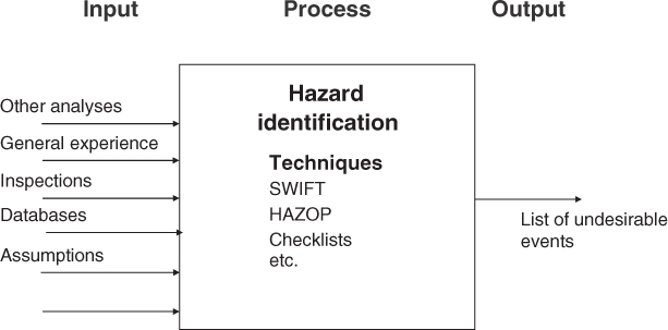
Figure 4.1 Hazard identification.

Several methods are available for carrying out such an identification process, and in Figure 4.1 various techniques/methods that can be used are listed. Failure Modes and Effects Analysis (FMEA), Hazard and Operability study (HAZOP) and Structured What-If Technique (SWIFT) are discussed in Chapter 6. A common feature of all these methods is that they are based on a type of structured brainstorming in which one uses checklists, guidewords and so on adapted to the problem being studied.

The hazard identification process should be a creative process wherein one also attempts to identify ‘unusual events’. Here, as in many other instances, a form of the 80–20 rule applies, i.e., it takes 20% of the time to come up with 80% of the hazards—events that we are familiar with and have experienced—while it takes 80% of the time to arrive at the remaining hazards and threats—the unusual and not-experienced events. It is to capture some of these last-mentioned events that it is so important to adopt a systematic and structured method.

4.2 Cause analysis

In the cause analysis, we study what is needed for the initiating events to occur. What are the causal factors? Several techniques exist for this purpose, from brainstorming sessions to fault tree analyses and Bayesian networks (see Chapter 6). In Figure 4.2, we have shown an example using fault trees. Experts on the systems and activities being studied are usually necessary to carry out the analysis. An in-depth understanding of the system is normally required.

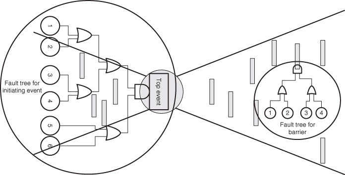
Figure 4.2 Use of fault trees.

In many cases, the analysis will consist of several ‘sub-risk analyses’. Let us return to the example ‘Disconnection from server’ discussed in Chapter 2. In the example, four different causes of the event ‘disconnection from server’ are identified. We look closer at one of them: power supply failure. For this new initiating event, we carry out a ‘new’ risk analysis. We study the causes and consequences, and a new bow-tie is established, as shown in Figure 4.3. In the consequence analysis, we are concerned with the consequences for the server, but the analysis will reveal consequences for other systems as well. This could provide a basis for assessing the need for measures that could reduce the probability of server failure, for example, labelling of cables and procedures for excavation and maintenance, or reduce the consequences of the event, for example, redundancy or having more in-lines following different routings.

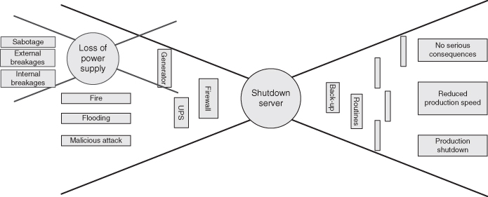
Figure 4.3 Cause analysis for disconnection from server (shutdown).

If we have access to failure data, then these can be used as a basis for predicting the number of times an event will occur. Such predictions can also be produced by using analysis methods such as fault tree analysis and Bayesian networks. If, for example, a fault tree analysis is used, one can assign probabilities for the various events in the tree (basic events), and based on the model and the assigned probabilities, the probability for the initiating event can be calculated (see Section 6.6).

4.3 Consequence analysis

For each initiating event, an analysis is carried out addressing the possible consequences the event can lead to. See the right side of Figure 4.3. An initiating event can often result in consequences of varying dimensions or attributes, for example, financial loss, loss of lives and environmental damage. The event tree analysis is the most common method for analysing the consequences. It will be thoroughly described in Section 6.7.

The number of steps in the event sequence is dependent on the number of barriers in the system. The aim of the consequence-reducing barriers is to prevent the initiating events from resulting in serious consequences. For each of these barriers, we can carry out barrier failure analysis and study the effect of measures taken. The fault tree analysis is often used for this purpose (see Figure 4.2). In the figure, the fault tree analysis is also used to analyse the causes triggering the initiating event.

Analyses of interdependencies between the various systems and barriers constitute an important part of the analysis. As an example, imagine that sensitive information is stored in an ICT system behind two password-protected security levels. Thus, an unauthorised user cannot gain access to the information even if he/she has access to the ‘outer’ security level. However, the user may find it impractical to remember many passwords, and he/she might therefore choose to use the same password for both security levels. An unauthorised user can then gain access to the sensitive information by using just one password. In this case, a dependency exists between the barriers (the same password). A solution for making the system more robust could be to make it impossible for a user to assign the same password for both security levels.

The consequence analysis deals, to a large extent, with understanding physical phenomena, and various types of models of the phenomena are used. Let us look at an example related to the initiating event ‘gas leakage’ on an offshore installation. These are some of the questions we will then try to answer:

• How will the gas dispersion be on the installation? In order to answer this question, we use gas dispersion models that simulate the gas under variouswind and ventilation conditions, leakage rates and so on.
• Will the gas form a combustible mixture? Will a combustible gas mixture reach an ignition source? Will the gas ignite? Will there be an explosion or a fire? The models used to study these questions take into account the location and number of ignition sources, such as pumps and compressors, and are based on the results from the gas dispersion models.
• How will a possible fire develop? In order to answer this question, the so-called CFD (Computational Fluid Dynamics) simulation is often used, which predicts the spread of a fire based on features of the area (geometry), volume of gas and so on.
• If the ignition produces an explosion, what will be the explosion pressure? Explosion-simulating models have been developed, which predict pressures and take into account the numerous factors that affect the outcome of such an event.

In such consequence analyses, the models used form an important part of the background knowledge. The probabilities assigned are conditional on the models used.

4.4 Probabilities and uncertainties

The analysis has so far provided a set of event chains (scenarios). However, how likely are these different scenarios and the associated consequences? Some scenarios can be very serious should they occur, but if the probability is low, they are not so critical.

Probabilities and expected values are used to express the risk. However, all types of uncertainties associated with what will be the consequences are not reflected through the probabilities. As discussed in Chapter 2, a risk description based on probabilities alone does not necessarily provide a sufficiently informative picture of the risk. The probabilities are conditional on a certain background knowledge, and in many cases, it is difficult to transform uncertainty to probability figures. For a method to assess the strength of the background knowledge, see Section 2.4.

In a simple consequence analysis, only one consequence value is specified, even though different outcomes are possible. This value is normally interpreted as the expected value should the initiating event occur. If such an approach is used, one must be aware that there is uncertainty about which consequences can occur. This problem is discussed in more detail in Sections 2.3 and 4.5.

Example

A firm installs and services telephone and data cables. There have been a number of events where such cables have been cut due to excavation work, and this has led to several companies being without telephone and internet connection for several days. As a part of a larger risk and vulnerability analysis, the undesirable event ‘breakage of buried cable’ is studied. A consequence analysis is conducted to describe the possible results of such cable breakages. The analysis concludes that the consequences could range from a few subscribers being without connection to rupture of the entire communication linkage between two large cities. The probability that the most serious incident would occur is calculated to be very low. If the analysis group restricts its attention to the expected consequences—that some companies will be without connection—specifies a probability for this event and carries this information further into the analysis, then an important aspect of the risk picture will not be captured, namely, that it is actually possible to have a complete rupture of the traffic between two large cities.

Reflection

How do we determine the initiating events?

The challenge is to select the initiating events that are such that

• they collectively cover the entire risk picture;
• the number is not too large;
• the consecutive modelling supports the objective of the analysis.

In a processing plant, process leakages are often selected as initiating events. If we had looked further backwards along the causal chains, it would have been difficult to cover all the relevant scenarios, and the number would have increased significantly. If we had looked forward along the consequence chains, for example, to process-related fires, we will be forced to condition on different leakage scenarios, which means that we in fact reintroduce leakages as the initiating events. For fires we have considerably less historical data than leakages; hence, a fire cause analysis is required. And such a cause analysis is preferably carried out by introducing leakage as the initiating event. Alternatively, we may adopt a backwards approach as mentioned in Section 3.2, where leakages that could lead to a specific fire scenario are identified.

We conclude that the analysis is simpler and more structured if we choose to use leakage as the initiating event. However, what is the best choice is of course dependent on the objectives of the analysis.

4.5 Risk picture: risk presentation

The risk picture is established based on the cause analysis and the consequence analysis. The picture covers , where refers to the specified initiating events, the defined consequences, the probabilities that express how likely various events and outcomes are and is the background knowledge on which , and are based. In Chapters 7–13, we provide a number of examples showing this picture in various situations. See also Chapter 2. Generally, the risk picture will cover

• predictions (often expected values) of the quantities we are interested in (e.g. costs, number of fatalities);
• probability distributions, for example, related to costs and number of fatalities;
• strength of knowledge.
• manageability factors.

Depending on the objective and the type of analysis, the risk picture can be limited to some defined areas and issues. Let us look at an example.

Example

Assume that a consequence analysis is carried out for the undesirable event ‘shutdown of system S’, where system S is an ICT system that is used during surgical interventions at a hospital. Based on experience, it is expected that system S will shut down once every year. Until now, this has not led to serious consequences for the patients, but the staff at the hospital acknowledge that the consequences could be serious under slightly different circumstances. This is the background for conducting a consequence analysis.

There are uncertainties about the consequences of shutdown of system S. As a simplification, the various outcomes are divided into five categories. The uncertainty about what will happen if system S shuts down is quantified by means of probabilities, as shown in Figure 4.4. We see that these probabilities add up to 100%; hence, if the initiating event occurs, then one of these consequences must take place.

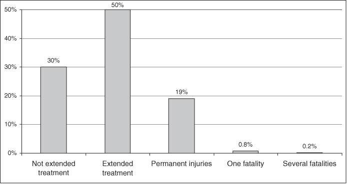
Figure 4.4 Probability of various consequences should the undesirable event occur.

The figure shows that shutdown of system S will most likely bring about extended treatment for some patients, but the event can lead to a spectrum of consequences ranging all the way from insignificant consequences to death of several patients. The initiating (undesirable) event can lead to consequences of varying seriousness, as showns in the figure.

The probabilities indicate how likely it is that the consequence will be ‘not extended treatment’, ‘extended treatment’ and so on. If we choose to present the probability—consequence dimensions in a risk matrix, how should we do this? A common method is to present the expected consequence of the event, that is, , where we, as mentioned earlier, denote the consequence by and the event by . The expected value is, in principle, the centre of gravity in Figure 4.4. However, since the consequence categories are described by text and not numbers, we cannot calculate this centre point mathematically. Furthermore, to compare the extended treatment with number of deaths is to integrate consequences having different dimensions. A ‘typical’ solution will be to use the consequence ‘extended treatment’ as the expected value, since this consequence corresponds to an approximate centre in the figure, with 30% of the probability mass on the one side and 20% on the other side. The expected consequence of the undesirable event is indicated by the triangular symbol in the risk matrix in Figure 4.5.

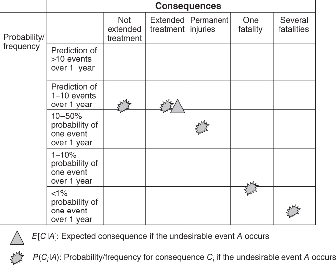
Figure 4.5 Example of a risk matri4.

From the example, we see that a risk description based on expected values does not give a particularly good picture of the risk. The consequence spectrum is not revealed. However, it is also possible to plot the consequence categories instead of the expected value. We then plot the points from Figure 4.4 directly:

• Not extended treatment: 30% probability
• Extended treatment: 50% probability
• Permanent injury: 19% probability
• One fatality: 0.8% probability
• Several fatalities: 0.2% probability.

These points are plotted in Figure 4.5 by using star-shaped symbols. This method of presenting the risk provides a more nuanced picture, since we show the range of different potential consequences, rather than just the expected consequences.

On the other hand, the volume of information can become too large when one tries to differentiate between all possible consequences. Using just one point makes it easier to compare risk contributions for the different events. The result is that in practice many are using the risk matrix based on , even though it can give a misleading picture of the risk.

The difference in the two methods used to plot the risk corresponds to the difference in Figures 2.1 and 2.2. If an event is located high to the right, the risk is high, whereas it is low if placed low to the left. Whether or not the risk is considered too high or acceptable is another issue. One often sees that the risk matrix is subdivided into three areas, upwards to the right indicates unacceptable risk, below to the left is the negligible risk zone and the middle zone is the ALARP area where the risks should be reduced to a level that is as low as reasonably practicable. We do not, however, use such a subdivision in this book, since we are, in principle, sceptical about the use of such pre-defined risk acceptance limits. See the discussion in Section 13.3.3. What is a tolerable risk and an acceptable risk cannot be considered in isolation from other considerations, for example, costs. On the other hand, it could be appropriate to have established standards or reference values that can tell what typically are the high and low values for the risk. In this way, it is much easier to sort out what is important and what is not.

Of importance in this context is the recognition that risk is more than just the numbers in the risk matri4. All probabilities and expected values are characterised by a certain background knowledge . The probability should be written . The background knowledge is a part of the risk picture and the risk presentation. We return to the issue in Section 4.5.1.

The above example shows the importance of looking at uncertainties beyond the expected values. We have repeatedly pointed out that it is necessary to look beyond the probabilities and expected values in order to view all aspects of uncertainty. The probabilities are not perfect tools for expressing uncertainty. The assumptions can hide important aspects of risk and uncertainty, and our lack of knowledge may lead to probabilities and expectations resulting in poor predictions. We shall see more examples of this in Chapters 7–13.

4.5.1 Handling the background knowledge

The risk description is conditional on the background knowledge as discussed in Chapter 2. This also applies to risk matrices, such as Figure 4.5. To reflect the strength of the background knowledge, we could perform an assessment as outlined in Section 2.4 and obtain an adjusted risk matrix as shown in Figure 2.6. We may for example show a risk matrix in which all the points in Figure 2.6 are to be understood as having a strong background knowledge except the one for several fatalities where the symbol is dashed to indicate that the background knowledge is considered to be of a medium strength.

Let us consider another example. You are carrying out a risk analysis of an offshore installation. The first part of the analysis is identification of initiating events. During the course of the process, a number of assumptions are made regarding operational conditions, certain risk-reducing measures that are in place, a certain manning level and so on.

Later on, a model-based risk analysis of an initiating event, ‘leakage in a gas line into the first-stage separator’, is carried out. In this analysis, assumptions are made regarding pressure, temperature, composition, which valves are open/closed, how often valves are tested, how long it would take for valves to close, the level of personnel in the various sections of the platform, emergency preparedness routines and so on. Computer programmes are used to simulate the gas discharge rate and relevant fire and explosion development. The programmes make use of various models, which, in turn, are based on a number of conditions and assumptions. Some of these are built into the model, while others can be controlled by the person conducting the risk analysis.

In other words, many assumptions are made during the course of the analysis process. These assumptions must be documented in a systematic way, and they must be presented to those who use the risk analysis for decision-making. The results obtained from the risk analyses must be viewed in the light of the assumptions made. Operational personnel should be aware of these assumptions, and it is essential that the assumptions are incorporated into the maintenance programme and the emergency preparedness planning and so on. In practice, it is a challenge to achieve all this successfully.

Sensitivity and robustness analyses

The risk picture is not complete unless we have carried out sensitivity and robustness analyses. These analyses show to what extent the results are dependent on important conditions and assumptions, and what it takes for the conclusions to be changed.

The depth of such analyses will, of course, depend on the decision problem, the risks that are analysed and the available resources.

Sensitivity analysis can be carried out on both the causal and consequence sides of initiating events. In the analysis, we study how the calculated risk changes its direction in response to changes in the information that the analysis is based on, for example, the probabilities used in event trees or in fault trees. An example is shown in Figure 4.6. The figure shows the effect on individual risk of increasing the helicopter transport for an offshore oil and gas field.

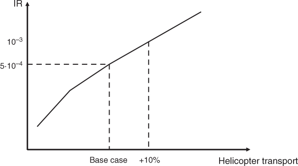
Figure 4.6 Example of sensitivity analysis.

In practice, we often start with the conclusion and ask what it takes for it to change. One can then ‘go backwards’ in the analysis and find out which conditions have a significant impact on the conclusion. We are talking about a robustness analysis. Carrying out sensitivity analyses on all conditions is not feasible in practice.

4.5.2 Risk evaluation

The discussion above has covered the key steps of a risk analysis, but it has also touched upon risk evaluation. Consider the discussion in the above example on what represents tolerable or acceptable risk. The risk evaluation will however be more thoroughly studied in the risk treatment discussion in Chapter 5. Through the risk analysis and the discussion of the results, the analysts will be able to give their message (the risk picture and the risk presentation), and then the management and decision-makers will become more central—we have entered the risk treatment chapter (Chapter 5).