7.3. Construction of Elementary Flows in Two Dimensions
In this section, elementary solutions of the Laplace equation are developed and then superimposed to produce a variety of geometrically simple ideal flows in two dimensions.
First, consider polynomial solutions of the Laplace equation in Cartesian coordinates. A zero-order polynomial, ψ or ϕ = constant, is not interesting since with either field function the result is u = 0. First-order polynomial solutions are given by (7.7) and (7.14), and these solutions represent spatially uniform velocity fields, u = (U,V). Quadratic functions in x and y are the next possibilities, and there are two of these:
 (7.24–7.27)
where A is a constant. (The reason for the two in (7.24) and (7.25) will be clear in the next section.) Here, only the flow field for 2Axy is constructed. Production of flow-field results for ψ and ϕ = A(x2 – y2) is left as an exercise.
Examine ψ = 2Axy first, and by direct differentiation find u = 2Ax, and v = –2Ay. Thus, for A > 0, the flow is toward the origin along the y-axis, away from it along the x-axis, and the streamlines are hyperbolae given by xy = ψ/2A (Figure 7.3). Considering the first quadrant only, this is ideal flow in a 90° corner. Now consider ϕ = 2Axy, and by direct differentiation find u = 2Ay, and v = 2Ax. The equipotential lines are hyperbolae given by xy = ϕ/2A. The flow is away from the origin along the line y = x and toward it along the line y = –x. Thus, ϕ = 2Axy produces a flow that is equivalent to that of ψ = 2Axy after a 45° rotation. Interestingly, higher-order polynomial solutions lead to flows in smaller-angle corners, while fractional powers lead to flows in larger-angle corners (see Section 4 and Exercises 7.8 and 7.9).
The next set of solutions to consider are (7.8) and (7.15) with x′= y′ = 0. In this case, curves of ψ = − ( Γ / 2 π ) ln x 2 + y 2 = const .  are circles centered on the origin of coordinates (Figure 7.4), and direct differentiation of (7.8) produces:
are circles centered on the origin of coordinates (Figure 7.4), and direct differentiation of (7.8) produces:
where r and θ are defined in Figure 3.3a. These results may be rewritten using the outcome of Example 2.2 as ur = 0 and uθ = Γ/2πr, which is the flow field of the ideal irrotational vortex (5.2). Similarly, curves of ϕ = ( q s / 2 π ) ln x 2 + y 2 = const .  are circles centered on the origin of coordinates (Figure 7.5), and direct differentiation of (7.15) produces:
are circles centered on the origin of coordinates (Figure 7.5), and direct differentiation of (7.15) produces: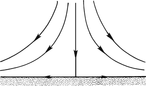
Figure 7.3 Stagnation point flow represented by ψ = 2Axy. Here, the flow impinges on the flat horizontal surface from above. The stagnation point is located where the single vertical streamline touches the horizontal surface.
These results may be rewritten as ur = qs/2πr and uθ = 0, which is purely radial flow away from the origin (Figure 7.5). Here, ∇ · u  is zero everywhere except at the origin. Thus, this potential represents flow from an ideal incompressible point source for qs > 0, or sink for qs < 0, that is located at r = 0 in two dimensions.
is zero everywhere except at the origin. Thus, this potential represents flow from an ideal incompressible point source for qs > 0, or sink for qs < 0, that is located at r = 0 in two dimensions.A source of strength +qs at (–ε, 0) and sink of strength –qs at (+ε, 0), can be considered together
to obtain the potential for a doublet in the limit that ε → 0  and
and q s → ∞  , so that the dipole strength vector:
and , so that the dipole strength vector: (7.28)


Figure 7.4 The flow field of an ideal vortex located at the origin of coordinates in two dimensions. The streamlines are circles and the potential lines are radials. Here, the vortex line is perpendicular to the x-y plane.
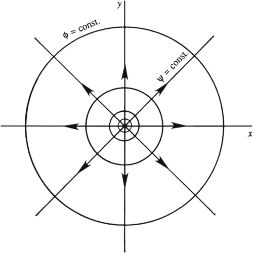
Figure 7.5 The flow field of an ideal source located at the origin of coordinates in two dimensions. The streamlines are radials and the potential lines are circles.


The doublet flow field is illustrated in Figure 7.6. The stream function for the doublet can be derived from (7.29) (Exercise 7.11).
The flows described by (7.7), (7.14), and (7.24) through (7.27) are solutions of the Laplace equation. The flows described by (7.8), (7.15), and (7.29) are singular at the origin and satisfy the Laplace equation for r > 0. Perhaps the most common and useful superposition of these solutions involves combining a uniform stream parallel to the x-axis, ψ = Uy or ϕ = Ux, and one or more of the singular solutions. The simplest example is the combination of a source and a uniform stream, which can be written in Cartesian and polar coordinates as:
 (7.30, 7.31)
Here the velocity field components are:
and streamlines are shown in Figure 7.7. The stagnation point is located at x = –a = –qs/2πU, and y = 0, and the value of the stream function on the stagnation streamline is ψ = qs/2.
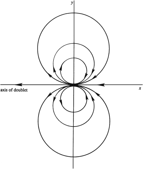
Figure 7.6 The flow field of an ideal two-dimensional doublet that points along the negative x-axis. The net source strength is zero so all streamlines begin and end at the origin. In this flow, the streamlines are circles tangent to the x-axis at the origin.
The streamlines that emerge vertically from the stagnation point (the darker curves in Figure 7.7) form a semi-infinite body with a smooth nose, generally called a half-body. These stagnation streamlines divide the field into regions external and internal to the half body. The internal flow consists entirely of fluid emanating from the source, and the external region contains fluid from upstream of the source. The half-body resembles several practical shapes, such as the leading edge of an airfoil or the front part of a bridge pier. The half-width of the body, h, can be found from (7.31) with ψ = qs/2:
The pressure distribution on the half body can be found from Bernoulli's equation, (7.18) with const. = p∞ + ρU2/2, and is commonly reported as a dimensionless excess pressure via the pressure coefficient Cp or Euler number (4.106):
 (7.32)
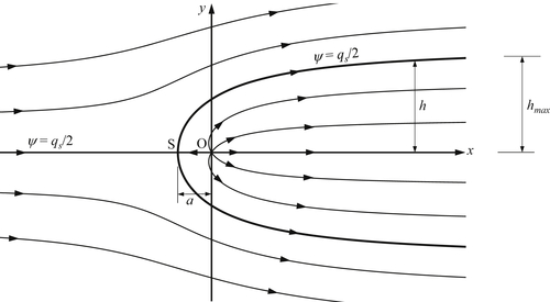
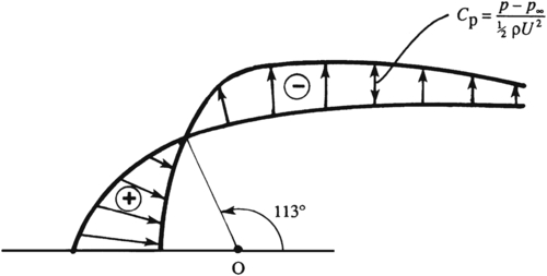
Figure 7.8 Pressure distribution in ideal flow over the half-body shown in Figure 7.7. Pressure excess near the nose is indicated by the circled “+” and pressure deficit elsewhere is indicated by the circled “–”.
A plot of Cp on the surface of the half-body is given in Figure 7.8, which shows that there is pressure excess near the nose of the body and a pressure deficit beyond it. Interestingly, integrating p over the surface leads to no net pressure force (see Exercise 7.15).
As a second example of flow construction via superposition, consider a horizontal free stream U and a doublet with strength d = –2πUa2ex:
 (7.33)
Here, ψ = 0 at r = a for all values of θ, showing that the streamline ψ = 0 represents a circular cylinder of radius a. The streamline pattern is shown in Figure 7.9 (and Figure 3.2a). In this flow, the net source strength is zero, so the cylindrical body is closed and does not extend downstream. The velocity field is:
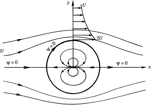
Figure 7.9 Ideal flow past a circular cylinder without circulation. This flow field is formed by combining a horizontal uniform stream flowing in the +x-direction with a doublet pointing in the –x-direction. The streamline that passes through the two stagnation points and forms the body surface is given by ψ = 0.

and this is shown by the continuous line in Figure 7.10. There are stagnation points on the cylinder’s surface at r-θ coordinates, (a, 0) and (a, π). The cylinder-surface pressure minima occur at r-θ coordinates (a, ±π/2) where the surface flow speed is maximum. The fore-aft symmetry of the pressure distribution implies that there is no net pressure force on the cylinder. In fact, a general result of two-dimensional ideal flow theory is that a steadily moving body experiences no drag. This result is at variance with observations and is sometimes known as d'Alembert's paradox. The existence of real-flow tangential stress on a solid surface, commonly known as skin friction, is not the only reason for the discrepancy. For blunt bodies such as a cylinder, most of the drag comes from flow separation and the formation of a wake, which is likely to be unsteady or even turbulent. When a wake is present, the flow loses fore-aft symmetry, and the surface pressure on the downstream side of the object is smaller than that predicted by ideal flow theory (Figure 7.10), resulting in pressure drag. These facts will be discussed in further in Chapter 10.
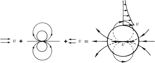
As discussed in Section 3.3, the flow due to a cylinder moving steadily through a fluid appears unsteady to an observer at rest with respect to the fluid at infinity. This flow is shown in Figure 3.2b and can be obtained by superposing a uniform stream in the negative x-direction with the flow shown in Figure 7.9. The resulting instantaneous streamline pattern is simply that of a doublet, as depicted by the decomposition shown in Figure 7.11.
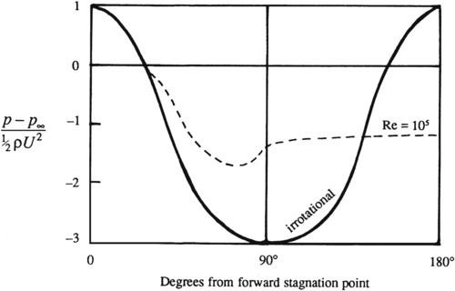
Figure 7.10 Comparison of irrotational and observed pressure distributions over a circular cylinder. Here 0° is the most upstream point of the cylinder and 180° is the most downstream point. The observed distribution changes with the Reynolds number; a typical behavior at high Re is indicated by the dashed line.
Although there is no net drag force on a circular cylinder in steady irrotational flow, there may be a lateral or lift force perpendicular to the free stream when circulation is added. Consider the flow field (7.33) with the addition of a point vortex of circulation −Γ1 at the origin that induces a clockwise velocity:
 (7.36)

Figure 7.12 Irrotational flow past a circular cylinder for different circulation values. Here S represents the stagnation point(s) in the flow. (a) At low values of the circulation, there are two stagnation points on the surface of the cylinder. (b) When the circulation is equal to 4πaU, there is one stagnation point on the surface of the cylinder. (c) When the circulation is even greater, there is one stagnation point below the cylinder.
Figure 7.12 shows the resulting streamline pattern for various values of Γ. The close streamline spacing and higher velocity on top of the cylinder is due to the addition of velocities from the clockwise vortex and the uniform stream. In contrast, the smaller velocities at the bottom of the cylinder are a result of the vortex field counteracting the uniform stream. Bernoulli's equation consequently implies a higher pressure below the cylinder than above it, and this pressure difference leads to an upward lift force on the cylinder.
The tangential velocity component at any point in the flow is:
At the surface of the cylinder, the fluid velocity is entirely tangential and is given by:
 (7.37)
which vanishes if:
 (7.38)
For Γ < 4πaU, two values of θ satisfy (7.38), implying that there are two stagnation points on the cylinder’s surface. The stagnation points progressively move down as Γ increases (Figure 7.12) and coalesce when Γ = 4πaU. For Γ > 4πaU, the stagnation point moves out into the flow along the negative y-axis. The radial distance of the stagnation point in this case is found from:

one root of which has r > a; the other root corresponds to a stagnation point inside the cylinder.
 (7.39)
The upstream-downstream symmetry of the flow implies that the pressure force on the cylinder has no stream-wise component. The vertical pressure force (per unit length perpendicular to the flow plane) is:

where n = er is the outward normal from the cylinder, and dl = adθ is a surface element of the cylinder’s cross section; L is known as the lift force in aerodynamics (Figure 7.13). Evaluating the integral using (7.39) produces:
 (7.40)
It is shown in Section 5 that (7.40) holds for irrotational flow around any two-dimensional object; it is not just for circular cylinders. The result that L is proportional to Γ is of fundamental importance in aerodynamics. Equation (7.40) was proved independently by the German mathematician, Wilhelm Kutta, and the Russian aerodynamist, Nikolai Zhukhovsky just after 1900; it is called the Kutta-Zhukhovsky lift theorem. (Older western texts transliterated Zhukhovsky's name as Joukowsky.) The interesting question of how certain two-dimensional shapes, such as an airfoil, develop circulation when placed in a moving fluid is discussed in Chapter 14. It is described there how fluid viscosity is responsible for the development of circulation. The magnitude of circulation, however, is independent of viscosity but does depend on the flow speed U, and the shape and orientation of the object.
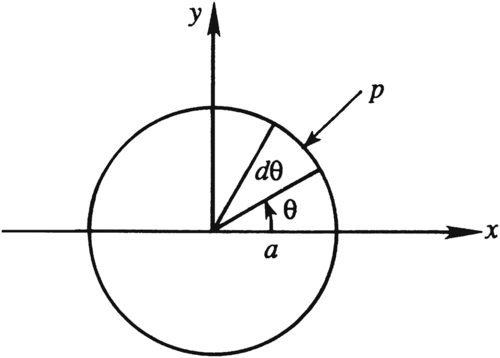
Figure 7.13 Calculation of pressure force on a circular cylinder. Surface pressure forces on top of the cylinder, where n has a positive vertical component, push the cylinder down. Thus the surface integral for the lift force applied by the fluid to the cylinder contains a minus sign.
For a circular cylinder, the only way to develop circulation is by rotating it. Although viscous effects are important in this case, the observed flow pattern for large values of cylinder rotation displays a striking similarity to the ideal flow pattern for Γ > 4πaU; see Figure 3.25 in the book by Prandtl (1952). For lower rates of cylinder rotation, the retarded flow in the boundary layer is not able to overcome the adverse pressure gradient behind the cylinder, leading to separation; the real flow is therefore rather unlike the irrotational pattern. However, even in the presence of separation, observed flow speeds are higher on the upper surface of the cylinder, implying a lift force.
A second reason for the presence of lift on a rotating cylinder is the flow asymmetry generated by a delay of boundary-layer separation on the upper surface of the cylinder. The contribution of this mechanism is small for two-dimensional objects such as the circular cylinder, but it is the only mechanism for side forces experienced by spinning three-dimensional objects like sports balls. The interesting question of why spinning balls follow curved paths is discussed in Section 10.9. The lateral force experienced by rotating bodies is called the Magnus effect.
Two-dimensional ideal flow solutions are commonly not unique and the topology of the flow domain determines uniqueness. Simply stated, a two-dimensional ideal flow solution is unique when any closed contour lying entirely within the fluid can be reduced to a point by continuous deformation without ever cutting through a flow-field boundary. Such fluid domains are singly connected. Thus, fluid domains, like those shown in Figures 7.9 and 7.12, that entirely encircle an object may not provide unique ideal flow solutions based on boundary conditions alone. In particular, consider the ideal flow (7.36) depicted in Figure 7.12 for various values of Γ. All satisfy the same boundary condition on the solid surface (ur = 0) and at infinity (u = Uex). The ambiguity occurs in these domains because there exist closed contours lying entirely within the fluid that cannot be reduced to a point, and on these contours a non-zero circulation can be computed. Fortunately, this ambiguity may often be resolved by considering real-flow effects. For example, the circulation strength that should be assigned to a streamlined object in two-dimensional ideal flow can be determined by applying the viscous-flow-based Kutta condition at the object’s trailing edge. This point is further explained in Chapter 14.
Another important consequence of the superposition principle for ideal flow is that it allows boundaries to be built into ideal flows through the method of images. For example, if the flow of interest in an unbounded domain is the solution of ∇ 2 ψ 1 = − ω 1 ( x , y )  , then
 ∇ 2 ψ 2 = − ω 1 ( x , y ) + ω 1 ( x , − y )  will determine the solution for the same vorticity distribution with a solid wall along the x-axis. Here,
 ψ 2 = ψ 1 ( x , y ) − ψ 1 ( x , − y )  , so that the zero streamline,
 ψ 2 = 0  , occurs on y = 0 (Figure 7.14). Similarly, if the flow of interest in an unbounded domain is the solution of
 ∇ 2 ϕ 1 = q 1 ( x , y )  , then
 ∇ 2 ϕ 2 = q 1 ( x , y ) + q 1 ( x , − y )  will determine the solution for the same source distribution with a solid wall along the x-axis. Here,
 ϕ 2 = ϕ 1 ( x , y ) + ϕ 1 ( x , − y )  so that
 v = ∂ ϕ 2 / ∂ y = 0  on y = 0 (Figure 7.15).
, then will determine the solution for the same vorticity distribution with a solid wall along the x-axis. Here, , so that the zero streamline, , occurs on y = 0 (Figure 7.14). Similarly, if the flow of interest in an unbounded domain is the solution of , then will determine the solution for the same source distribution with a solid wall along the x-axis. Here, so that on y = 0 (Figure 7.15).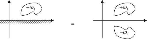
Figure 7.14 Illustration of the method of images for the flow generated by a vorticity distribution near a horizontal wall. An image distribution of equal strength and opposite sign mimics the effect of the solid wall.
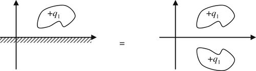
Figure 7.15 Illustration of the method of images for the flow generated by a source distribution near a horizontal wall. An image distribution of equal strength mimics the effect of the solid wall.
As an example of the method of images, consider the flow induced by an ideal source of strength qs a distance a from a straight vertical wall (Figure 7.16). Here an image source of the same strength and sign is needed a distance a on the other side of the wall. The stream function and potential for this flow are:
 (7.41)
After some rearranging and use of the two-angle formula for the tangent function, the equation for the streamlines may be found:

The x and y axes form part of the streamline pattern, with the origin as a stagnation point. This flow represents three interesting situations: flow from two equal sources (all of Figure 7.16), flow from a source near a flat vertical wall (right half of Figure 7.16), and flow through a narrow slit at x = a into a right-angled corner (first quadrant of Figure 7.16).
The method of images can sometimes be extended to circular boundaries by allowing more than one image vortex or source (Exercises 5.15, 7.28), and to unsteady flows as long as the image distributions of vorticity or source strength move appropriately. Unsteady two-dimensional ideal flow merely involves the inclusion of time as an independent variable in ψ or ϕ, and the addition of ρ(∂ϕ/∂t) in the Bernoulli equation (see Exercise 7.4). The following example, which validates the free-vortex results stated in Section 5.6, illustrates these changes.
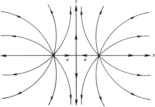
Figure 7.16 Ideal flow from two equal sources placed at x = ± a. The origin is a stagnation point. The vertical axis is a streamline and may be replaced by a solid surface. This flow field further illustrates the method of images.
At t = 0, an ideal free vortex with strength –Γ is located at point A near a flat solid vertical wall as shown in Figure 5.16. If the x,y-coordinates of A are (h,0) and the fluid far from the vortex is quiescent at pressure p∞, determine the trajectory ξ(t) = (ξx, ξy) of the vortex, and the pressure at the origin of coordinates as a function of time.
Solution
From the method of images, the stream function for this flow field will be:

The first term is for the image vortex and second term is for the original vortex. The horizontal and vertical components of the induced velocity for both vortices are:


[(4.83) with g = 0], where the second equality follows from evaluating the constant far from the vortex. Thus, at x = y = 0:
Here,