10

Type I and type II superstrings

Having spent volume one on a thorough development of the bosonic string, we now come to our real interest, the supersymmetric string theories. This requires a generalization of the earlier framework, enlarging the world-sheet constraint algebra. This idea arises naturally if we try to include spacetime fermions in the spectrum, and by guesswork we are led to superconformal symmetry. In this chapter we discuss the (1,1) superconformal algebra and the associated type I and II superstrings. Much of the structure is directly parallel to that of the bosonic string so we can proceed rather quickly, focusing on the new features.

10.1 The superconformal algebra

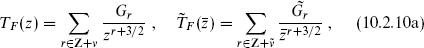
In bosonic string theory, the mass-shell condition

came from the physical state condition

and also from |ψ = 0 in the closed string. The mass-shell condition is the Klein–Gordon equation in momentum space. To get spacetime fermions, it seems that we need the Dirac equation

instead. This is one way to motivate the following generalization, and it will lead us to all the known consistent string theories.

Let us try to follow the pattern of the bosonic string, where L₀ and are the center-of-mass modes of the world-sheet energy-momentum tensor (T_B, ). A subscript B for ‘bosonic’ has been added to distinguish these from the fermionic currents now to be introduced. It seems then that we need new conserved quantities T_F and , whose center-of-mass modes give the Dirac equation, and which play the same role as T_B and in the bosonic theory. Noting further that the spacetime momenta p^μ are the center-of-mass modes of the world-sheet current (∂X^μ, X^μ), it is natural to guess that the gamma matrices, with algebra

are the center-of-mass modes of an anticommuting world-sheet field ψ^μ.

With this in mind, we consider the world-sheet action

For reference we recall from chapter 2 the XX operator product expansion (OPE)

The ψ conformal field theory (CFT) was described in section 2.5. The fields ψ^μ and are respectively holomorphic and antiholomorphic, and the operator products are

The world-sheet supercurrents

are also respectively holomorphic and antiholomorphic, since they are just the products of (anti)holomorphic fields. The annoying factors of (2/α′)^1/2 could be eliminated by working in units where α′ = 2, and then be restored if needed by dimensional analysis. Also, throughout this volume the : : normal ordering of coincident operators will be implicit.

This gives the desired result: the modes and will satisfy the gamma matrix algebra, and the centers-of-mass of T_F and will have the form of Dirac operators. We will see that the resulting string theory has spacetime fermions as well as bosons, and that the tachyon is gone.

From the OPE and the Ward identity it follows (exercise 10.1) that the currents

generate the superconformal transformation

This transformation mixes the commuting field X^μ with the anticommuting fields ψ^μ and , so the parameter η(z) must be anticommuting. As with conformal symmetry, the parameters are arbitrary holomorphic or antiholomorphic functions. That this is a symmetry of the action (10.1.5) follows at once because the current is (anti)holomorphic, and so conserved.

The commutator of two superconformal transformations is a conformal transformation,

as the reader can check by acting on the various fields. Similarly, the commutator of a conformal and superconformal transformation is a superconformal transformation. The conformal and superconformal transformations thus close to form the superconformal algebra. In terms of the currents, this means that the OPEs of T_F with itself and with

close. That is, only T_B and T_F appear in the singular terms:

and similarly for the antiholomorphic currents. The T_BT_F OPE implies that T_F is a tensor of weight . Each scalar contributes 1 to the central charge and each fermion , for a total

This enlarged algebra with T_F and as well as T_B and will play the same role that the conformal algebra did in the bosonic string. That is, we will impose it on the states as a constraint algebra — it must annihilate physical states, either in the sense of old covariant quantization (OCQ) or of Becchi–Rouet–Stora–Tyutin (BRST) quantization. Because of the Minkowski signature of spacetime the timelike ψ⁰ and , like X⁰, have opposite sign commutators and lead to negative norm states. The fermionic constraints T_F and will remove these states from the spectrum.

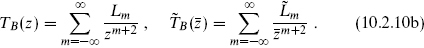
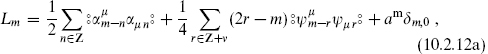
More generally, the N = 1 superconformal algebra in operator product form is

The Jacobi identity requires the same constant c in the T_BT_B and T_FT_F products (exercise 10.5). Here, N = 1 refers to the number of currents. In the present case there is also an antiholomorphic copy of the same algebra, so we have an (N, Ñ) = (1, 1) superconformal field theory (SCFT). We will consider more general algebras in section 11.1.

Free SCFTs

The various free CFTs described in chapter 2 have superconformal generalizations. One free SCFT combines an anticommuting bc theory with a commuting βγ system, with weights

The action is

and

The central charge is

Of course there is a corresponding antiholomorphic theory.

We can anticipate that the superconformal ghosts will be of this form with λ = 2, the anticommuting (2, 0) ghost b being associated with the commuting (2, 0) constraint T_B as in the bosonic theory, and the commuting ghost β being associated with the anticommuting constraint T_F. The ghost central charge is then −26 + 11 = −15, and the condition that the total central charge vanish gives the critical dimension

For λ = 2,

Another free SCFT is the superconformal version of the linear dilaton theory. This has again the action (10.1.5), while

each having an extra term as in the bosonic case. The reader can verify that these satisfy the N = 1 algebra with

10.2 Ramond and Neveu–Schwarz sectors

We now study the spectrum of the X^μψ^μ SCFT on a circle. Much of this is as in chapter 2, but the new ingredient is a more general periodicity condition. It is clearest to start with the cylindrical coordinate w = σ¹+iσ². The matter fermion action

must be invariant under the periodic identification of the cylinder, w ≅ w + 2π. This condition plus Lorentz invariance still allows two possible periodicity conditions for ψ^μ,

where the sign must be the same for all μ. Similarly there are two possible periodicities for . Summarizing, we will write

where ν and take the values 0 and .

Since we are initially interested in theories with the maximum Poincaré invariance, X^μ must be periodic. (Antiperiodicity of X^μ is interesting, and we have already encountered it for the twisted strings on an orbifold, but it would break some of the translation invariance.) The supercurrent then has the same periodicity as the corresponding ψ,

Thus there are four different ways to put the theory on a circle, each of which will lead to a different Hilbert space — essentially there are four different kinds of closed superstring. We will denote these by (ν, ) or by NS–NS, NS–R, R–NS, and R–R. They are analogous to the twisted and untwisted sectors of the Z₂ orbifold. Later in the chapter we will see that consistency requires that the full string spectrum contain certain combinations of states from each sector.

To study the spectrum in a given sector expand in Fourier modes,

the phase factors being inserted to conform to convention later. On each side the sum runs over integers in the R sector and over (integers + ) in the NS sector. Let us also write these as Laurent expansions. Besides replacing exp(−iw) → z we must transform the fields,

The clumsy subscripts are a reminder that these transform with half the weight of a vector. Henceforth the frame will be indicated implicitly by the argument of the field. The Laurent expansions are then

Notice that in the NS sector, the branch cut in z^−1/2 offsets the original antiperiodicity, while in the R sector it introduces a branch cut. Let us also recall the corresponding bosonic expansions

where in the closed string and in the open string.

The OPE and the Laurent expansions (or canonical quantization) give the anticommutators

For T_F and T_B the Laurent expansions are

The usual CFT contour calculation gives the mode algebra

This is known as the Ramond algebra for r, s integer and the Neveu–Schwarz algebra for r, s half-integer. The antiholomorphic fields give a second copy of these algebras.

The superconformal generators in either sector are

Again denotes creation–annihilation normal ordering. The normal ordering constant can be obtained by any of the methods from chapter 2; we will use here the mnemonic from the end of section 2.9. Each periodic boson contributes −. Each periodic fermion contributes + and each antiperiodic fermion −. Including the shift +c = D gives

For the open string, the condition that the surface term in the equation of motion vanish allows the possibilities

By the redefinition 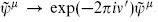, we can set ν′ = 0. There are therefore two sectors, R and NS, as compared to the four of the closed string. To write the mode expansion it is convenient to combine ψ^μ and into a single field with the extended range 0 ≤ σ¹ ≤ 2π. Define

for π ≤ σ¹ ≤ 2π. The boundary condition ν′ = 0 is automatic, and the antiholomorphicity of implies the holomorphicity of the extended ψ^μ. Finally, the boundary condition (10.2.14) at σ¹ = 0 becomes a periodicity condition on the extended ψ^μ, giving one set of R or NS oscillators and the corresponding algebra.

NS and R spectra

We now consider the spectrum generated by a single set of NS or R modes, corresponding to the open string or to one side of the closed string. The NS spectrum is simple. There is no r = 0 mode, so we define the ground state to be annihilated by all r > 0 modes,

The modes with r < 0 then act as raising operators; since these are anticommuting, each mode can only be excited once.

The main point of interest is the R ground state, which is degenerate due to the s. Define the ground states to be those that are annihilated by all r > 0 modes. The satisfy the Dirac gamma matrix algebra (10.1.4) with

Since for r > 0, the take ground states into ground states. The ground states thus form a representation of the gamma matrix algebra. This representation is worked out in section B.1; in D = 10 it has dimension 32. The reader who is not familiar with properties of spinors in various dimensions should read section B.1 at this point. We can take a basis of eigenstates of the Lorentz generators S_a, eq. (B.1.10):

The half-integral values show that these are indeed spacetime spinors. A more general basis for the spinors would be denoted |α_R. In the R sector of the open string not only the ground state but all states have half-integer spacetime spins, because the raising operators are vectors and change the S_a by integers. In the NS sector, the ground state is annihilated by S^μν and is a Lorentz singlet, and all other states then have integer spin.

The Dirac representation 32 is reducible to two Weyl representations 16 + 16′, distinguished by their eigenvalue under Γ as in eq. (B.1.11). This has a natural extension to the full string spectrum. The distinguishing property of Γ is that it anticommutes with all Γ^μ. Since the Dirac matrices are now the center-of-mass modes of ψ^μ, we need an operator that anticommutes with the full ψ^μ. We will call this operator

where F, the world-sheet fermion number, is defined only mod 2. Since ψ^μ changes F by one it anticommutes with the exponential. It is convenient to write F in terms of spacetime Lorentz generators, which in either sector of the ψ CFT are

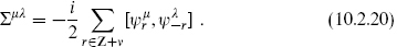
This is the natural extension of the zero-mode part (B.1.8). Define now

the i being included to make S₀ Hermitean, and let

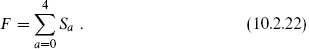
This has the desired property. For example,

so these oscillators change F by ±1. The definition (10.2.22) makes it obvious that F is conserved by the OPE of the vertex operators, as a consequence of Lorentz invariance.¹ When we include the ghost part of the vertex operator in section 10.4, we will see that it contributes to the total F, so that on the total matter plus ghost ground state one has

The ghost ground state contributes a factor −1 in the NS sector and −i in the R sector.

Closed string spectra

In the closed string, the NS–NS states have integer spin. Because the spins S_a are additive, the half-integers from the two sides of the R–R sector also combine to give integer spin. The NS–R and R–NS states, on the other hand, have half-integer spin.

Let us look in more detail at the R–R sector, where the ground states |s, s′_R are degenerate on both the right and left. They transform as the product of two Dirac representations, which is worked out in section B.1:

where [n] denotes an antisymmetric rank n tensor. For the closed string there are separate world-sheet fermion numbers F and , which on the ground states reduce to the chirality matrices Γ and acting on the two sides. The ground states thus decompose as in table 10.1.

Table 10.1. SO(9, 1) representations of massless R–R states.

10.3 Vertex operators and bosonization

Consider first the unit operator. Fields remain holomorphic at the origin, and in particular they are single-valued. From the Laurent expansion (10.2.7), the single-valuedness means that the unit operator must be in the NS sector; the conformal transformation that takes the incoming string to the point z = 0 cancels the branch cut from the antiperiodicity. The holomorphicity of ψ at the origin implies, via the contour argument, that the state corresponding to the unit operator satisfies

and therefore

Since the ψψ OPE is single-valued, all products of ψ and its derivatives must be in the NS sector. The contour argument gives the map

so that there is a one-to-one map between such products and NS states. The analog of the Noether relation (2.9.6) between the superconformal variation of an NS operator and the OPE is

The R sector vertex operators must be more complicated because the Laurent expansion (10.2.7) has a branch cut. We have encountered this before, for the winding state vertex operators in section 8.2 and the orbifold twisted state vertex operators in section 8.5. Each of these introduces a branch cut (the first a log and the second a square root) into X^μ. For the winding state vertex operators there was a simple expression as the exponential of a free field. For the twisted state vertex operators there was no simple expression and their amplitudes are determined only with more effort. Happily, through a remarkable property of two-dimensional field theory, the R sector vertex operators can be related directly to the bosonic winding state vertex operators.

Let H(z) be the holomorphic part of a scalar field,

For world-sheet scalars not associated directly with the embedding of the string in spacetime this is the normalization we will always use, corresponding to α′ = 2 for the embedding coordinates. As in the case of the winding state vertex operators we can be cavalier about the location of the branch cut as long as the final expressions are single-valued. We will give a precise oscillator definition below. Consider the basic operators e^±iH(z). These have the OPE

The poles and zeros in the OPE together with smoothness at infinity determine the expectation values of these operators on the sphere, up to an overall normalization which can be set to a convenient value:

The are ±1 here, but this result holds more generally.

Now consider the CFT of two Majorana–Weyl fermions ψ^{1, 2}(z), and form the complex combinations

These have the properties

Eqs. (10.3.6) and (10.3.9) are identical in form, and so the expectation values of ψ(z) on the sphere are identical to those of e^iH(z). We will write

to indicate this. Of course, all of this extends to the antiholomorphic case,

Since arbitrary local operators with integral k_R and k_L can be formed by repeated operator products of e^±iH(z) and , and arbitrary local operators built out of the fermions and their derivatives can be formed by repeated operator products of , the equivalence of the theories can be extended to all local operators. Finally, in order for these theories to be the same as CFTs, the energy-momentum tensors must be equivalent. The easiest way to show this is via the operator products

With the result (10.3.10), this implies equivalence of the H momentum current with the ψ number current, and of the two energy-momentum tensors,

As a check, e^iH and ψ are both tensors.

In the operator description of the theory, define

From the Campbell–Baker–Hausdorff (CBH) formula (6.7.23) we have for equal times |z| = |z′|

where we have used the fact (8.2.21) that at equal times [H(z), H(z′)] = ±iπ. Thus the bosonized operators do anticommute. This is possible for operators constructed purely out of bosons because they are nonlocal. In particular, note that the CBH formula gives the equal time commutator

so that the fermion field operator produces a kink, a discontinuity, in the bosonic field.

This rather surprising equivalence is known as bosonization. Equivalence between field theories with very different actions and fields occurs frequently in two dimensions, especially in CFTs because holomorphicity puts strong constraints on the theory. (The great recent surprise is that it is also quite common in higher-dimensional field and string theories.) Many interesting CFTs can be constructed in several different ways. One form or another will often be more useful for specific purposes. Notice that there is no simple correspondence between one-boson and one-fermion states. The current, for example, is linear in the boson field but quadratic in the fermion field. A single boson is the same as one ψ fermion and one fermion at the same point. On a Minkowski world-sheet, where holomorphic becomes left-moving, the fermions both move left at the speed of light and remain coincident, indistinguishable from a free boson. A single fermion, on the other hand, is created by an operator exponential in the boson field and so is a coherent state, which as we have seen is in the shape of a kink (10.3.16).

The complicated relationship between the bosonic and fermionic spectra shows up also in the partition function. Operator products of e^±iH(z) generate all operators with integer k_L. The bosonic momentum and oscillator sums then give

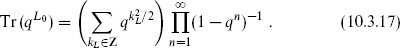
In the NS sector of the fermionic theory, the oscillator sum gives

We know indirectly that these must be equal, since we can use the OPE to construct an analog in the fermionic theory for any local operator of the bosonic theory and vice versa. Expanding the products gives

for each, and in fact the equality of (10.3.17) and (10.3.18) follows from the equality of the product and sum expressions for theta functions, section 7.2. Note that while bosonization was derived for the sphere, the sewing construction from chapter 9 guarantees that it holds on all Riemann surfaces, provided that we make equivalent projections on the spectra. In particular, we have seen that summing over integer k_L corresponds to summing over all local fermionic operators, the NS sector.

Bosonization extends readily to the R sector. In fact, once we combine two fermions into a complex pair we can consider the more general periodicity condition

for any real ν. In ten dimensions only ν = 0, arose, but these more general periodicities are important in less symmetric situations. The Laurent expansion has the same form (10.2.7) as before,

with indices displaced from integers by ±ν. The algebra is

Define a reference state |0_ν by

The first nonzero terms in the Laurent expansions are then r = − 1 + ν and s = −ν, so for the corresponding local operator the OPE is

The conditions (10.3.23) uniquely identify the state |0_ν, and so the corresponding OPEs (10.3.24) determine the bosonic equivalent

One can check the identification (10.3.25) by verifying that the weight is . In the bosonic form this comes from the term p² in L₀. In the fermionic form it follows from the usual commutator method (2.7.8) or the zero-point mnemonic.

The boundary condition (10.3.20) is the same for ν and ν + 1, but the reference state that we have defined is not. It is a ground state only for 0 ≤ ν ≤ 1. As we vary ν, the state |0_ν changes continuously, and when we get back to the original theory at ν + 1, by the definition (10.3.23) it has become the excited state

This is known as spectral flow. For the R case ν = 0 there are the two degenerate ground states

For the superstring in ten dimensions we need five bosons, H^a for a = 0, …, 4. Then²

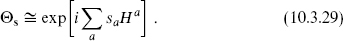
The vertex operator Θ_s for an R state |s is

This operator, which produces a branch cut in ψ^μ, is sometimes called a spin field. For closed string states, this is combined with the appropriate antiholomorphic vertex operator, built from .

The general bc CFT, renaming ψ → b and → c, is obtained by modifying the energy-momentum tensor of the λ = theory to

The equivalences (10.3.13) give the corresponding bosonic operator

This is the same as the linear dilaton CFT, with V = −i(λ − ). With this correspondence between V and λ, the linear dilaton and bc theories are equivalent,

As a check, the central charges agree,

So do the dimensions of the fields (10.3.32), λ for b and 1−λ for c, agreeing with k²/2 + ikV for e^ikH. The nontensor behaviors of the currents bc and i∂H are also the same. Since the inner product for the reparameterization ghosts makes b and c Hermitean, the bosonic field H must be anti-Hermitean in this application. The bosonization of the ghosts is usually written in terms of a Hermitean field with the opposite sign OPE,

10.4 The superconformal ghosts

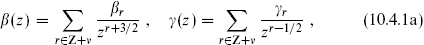
To build the BRST current we will need, in addition to the anticommuting b and c ghosts of the bosonic string, commuting ghost fields β and γ of weight and (− , 0), and the corresponding antiholomorphic fields. The action for this SCFT was given in eq. (10.1.17) and the currents T_B and T_F in eq. (10.1.21). The ghosts β and γ must have the same periodicity (10.2.4) as the generator T_F with which they are associated. This is necessary to make the BRST current periodic, so that it can be integrated to give the BRST charge. Thus,

and similarly for the antiholomorphic fields. The (anti)commutators are

Define the ground states |0_NS,R by

We have grouped β₀ with the lowering operators and γ₀ with the raising ones, in parallel with the bosonic case. The spectrum is built as usual by acting on the ground states with the raising operators. The generators are

The normal ordering constant is determined by the usual methods to be

Vertex operators

We focus here on the βγ CFT, as the bc parts of the vertex operators are already understood. Let us start by considering the state corresponding to the unit operator. From the Laurent expansions (10.4.1) it is in the NS sector and satisfies

This is not the same as the ground state |0_NS: the mode γ_1/2 annihilates |0_NS while its conjugate β_−1/2 annihilates |1. We found this also for the bc ghosts with c₁ and b₋₁. Since anticommuting modes generate just two states, we had the simple relation |0 = c₁|1 (focusing on the holomorphic side). For commuting oscillators things are not so simple: there is no state in the Fock space built on |1 by acting with γ_1/2 that has the properties of |0_NS. The definition of the state |0_NS translates into

for the corresponding operator δ(γ). The notation δ(γ) reflects the fact that the field γ has a simple zero at the vertex operator. Recall that for the bc ghosts the NS ground state maps to the operator c, which is the anticommuting analog of a delta function. One can show that an insertion of δ(γ) in the path integral has the property (10.4.7).

To give an explicit description of this operator it is again convenient to bosonize. Of course β and γ are already bosonic, but bosonization here refers to a rewriting of the theory in a way that is similar to, but a bit more intricate than, the bosonization of the anticommuting bc theory.

Start with the current βγ. The operator product

is the same as that of ∂, where (z)(0) ∼ − ln z is a holomorphic scalar. Holomorphicity then implies that this equivalence extends to all correlation functions,

The OPE of the current with β and γ then suggests

For the bc system we would be finished: this approach leads to the same bosonization as before. For the βγ system, however, the sign of the current–current OPE and therefore of the OPE is changed. The would-be bosonization (10.4.10) gives the wrong OPEs: it would imply

whereas the correct OPE is

To repair this, additional factors are added,

In order not to spoil the OPE with the current (10.4.9), the new fields η(z) and ξ(z) must be nonsingular with respect to , which means that the ηξ theory is a new CFT, decoupled from the CFT. Further, the equivalence (10.4.13) will hold — all OPEs will be correct — if η and ξ satisfy

This identifies the ηξ theory as a holomorphic CFT of the bc type: the OPE of like fields has a zero due to the anticommutativity.

It remains to study the energy-momentum tensor. We temporarily consider the general βγ system, with β having weight λ′. The OPE

determines the energy-momentum tensor,

The exponentials in the bosonization (10.4.13) thus have weights λ′ − 1 and −λ′ respectively, as compared with the weights λ′ and 1 − λ′ of β and γ. This fixes the weights of η and ξ as 1 and 0: this is a λ = 1 bc system, with

and

As a check, the central charges are 3(2λ′ − 1)² + 1 for and −2 for , adding to the 3(2λ′ − 1)² − 1 of the βγ CFT. The need for extra degrees of freedom is not surprising. The βγ theory has a greater density of states than the bc theory because the modes of a commuting field can be excited any number of times. One can check that the total partition functions agree, in the appropriate sectors.

If need be one can go further and represent the ηξ theory in terms of a free boson, conventionally χ with χ(z)χ(0) ∼ ln z, as in the previous section. Thus

The energy-momentum tensor is then

For the string, the relevant value is λ′ = . The properties (10.4.7) of δ(γ) determine the bosonization,

The fermionic parts of the tachyon and massless NS vertex operators are then

respectively. For λ′ = , the exponential e^l has weight − l² − l.

The operator Σ corresponding to |0_R satisfies

This determines

Adding the contribution −1 of the bc ghosts, the weight of e^−/2 and of e⁻ agree with the values (10.4.5). The R ground state vertex operators are then

with the spin field Θ_s having been defined in eq. (10.3.29).

We need to extend the definition of world-sheet fermion number F to be odd for β and γ. The ultimate reason is that it anticommutes with the supercurrent T_F and we will need it to commute with the BRST operator, which contains terms such as γT_F. The natural definition for F is then that it be the charge associated with the current (10.4.9), which is l for e^l. Again, it is conserved by the OPE. This accounts for the ghost contributions in eq. (10.2.24). Note that this definition is based on spin rather than statistics, since the ghosts have the wrong spin-statistics relation; it would therefore be more appropriate to call F the world-sheet spinor number.

For completeness we give a general expression for the cocycle for exponentials of free fields, though we emphasize that for most purposes the details are not necessary. In general one has operators

with the holomorphic and antiholomorphic scalars not necessarily equal in number. The momenta k take values in some lattice Γ. The naive operator product has the phase of z^{−k ○ k′}, and for all pairs in Γ, k ○ k′ must be an integer. The notation is as in section 8.4, . When k ○ k′ is an odd integer the vertex operators anticommute rather than commute. A correctly defined vertex operator is

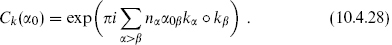
with the cocycle C_k defined as follows. Take a set of basis vectors k_α for Γ; that is, Γ consists of the integer linear combinations n_αk_α. Similarly write the vector of zero-mode operators in this basis, α₀ = α_0αk_α, Then for k = n_αk_α,

This generalizes the simple case (8.2.22). The reader can check that vertex operators with even k ○ k now commute with all vertex operators, and those with odd k ○ k anticommute among themselves. Note that a cocycle has no effect on the commutativity of a vertex operator with itself, so an exponential must be bosonic if k o k is even and fermionic if k ○ k is odd.

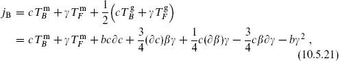
10.5 Physical states

In the bosonic string we started with a (diff×Weyl)-invariant theory. After fixing to conformal gauge we had to impose the vanishing of the conformal algebra as a constraint on the states. In the present case there is an analogous gauge-invariant form, and the superconformal algebra emerges as a constraint in the gauge-fixed theory. However, it is not necessary to proceed in this way, and it would require us to develop some machinery that in the end we do not need. Rather we can generalize directly in the gauge-fixed form, defining the superconformal symmetry to be a constraint and proceeding in parallel to the bosonic case to construct a consistent theory. We will first impose the constraint in the old covariant formalism, and then in the BRST formalism.

OCQ

In this formalism, developed for the bosonic string in section 4.1, one ignores the ghost excitations. We begin with the open string, imposing the physical state conditions

Only the matter part of any state is nontrivial — the ghosts are in their ground state — and the superscript ‘m’ denotes the matter part of each generator. There are also the equivalence relations

The mass-shell condition can always be written in terms of the total matter plus ghost Virasoro generator, which is the same as the world-sheet Hamiltonian H because the total central charge is zero:

In ten flat dimensions this is

The zero-point constants from the ghosts and longitudinal oscillators have canceled as usual, leaving the contribution of the transverse modes,

For the tachyonic and massless levels we need only the terms

The NS sector works out much as in the bosonic string. The lowest state is |0; k_NS, labeled by the matter state and momentum. The only nontrivial condition is from L₀, giving

This state is a tachyon. It has exp(πiF) = −1, where F was given in eq. (10.2.24). The first excited state is

The nontrivial physical state conditions are

while

is null. Thus

This state is massless, the half-unit of excitation canceling the zero-point energy, and has exp(πiF) = +1. Like the first excited state of the bosonic string it is a massless vector, with D − 2 spacelike polarizations. The constraints have removed the unphysical polarizations of ψ^μ, just as for X^μ in the bosonic case.

In the R sector the lowest states are

Here u_s is the polarization, and the sum on s is implicit. The nontrivial physical state conditions are

The ground states are massless because the zero-point energy vanishes in the R sector. The condition gives the massless Dirac equation

which was our original goal in introducing the superconformal algebra. The condition implies the L₀ condition, because in the critical dimension and the ghost parts of G₀ annihilate the ghost vacuum.

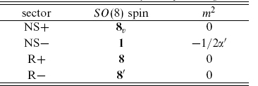
In ten dimensions, massless particle states are classified by their behavior under the SO(8) rotations that leave the momentum invariant. Take a frame with k₀ = k₁. In the NS sector, the massless physical states are the eight transverse polarizations forming the vector representation 8_v of SO(8). In the R sector, the massless Dirac operator becomes

The physical state condition is then

so precisely the states with s₀ = + survive. As discussed in section B.1, we have under SO(9, 1) → SO(1, 1) × SO(8) the decompositions

Thus the Dirac equation leaves an 8 with exp(πiF) = +1 and an 8′ with exp(πiF) = −1.

The tachyonic and massless states are summarized in table 10.2. The open string spectrum has four sectors, according to the periodicity ν and the world-sheet fermion number exp(πiF). We will use the notation NS± and R± to label these sectors. We will see in the next section that consistency requires us to keep only certain subsets of sectors, and that there are consistent string theories without the tachyon.

Table 10.2. Massless and tachyonic open string states.

Closed string spectrum

The closed string is two copies of the open string, with the momentum rescaled k → k in the generators. With ν, taking the values 0 and , the mass-shell condition can be summarized as

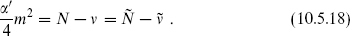
The tachyonic and massless closed string spectrum is obtained by combining one left-moving and one right-moving state, subject to the equality (10.5.18).

The (NS−,NS−) sector contains a closed string tachyon with m² = −2/α′. At the massless level, combining the various massless left- and right-moving states from table 10.2 leads to the SO(8) representations shown in table 10.3. Note that level matching prevents pairing of the NS− sector with any of the other three. As in the bosonic string, vector times vector decomposes into scalar, antisymmetric tensor, and traceless symmetric tensor denoted (2). The products of spinors are discussed in section B.1.

Table 10.3. Products of SO(8) representations appearing at the massless level of the closed string. The R–NS sector has the same content as the NS–R sector.

The 64 states in 8_v × 8 and 8_v × 8′ each separate into two irreducible representations. Denoting a state in 8_v × 8 by |i, s, we can form the eight linear combinations

These states transform among themselves under SO(8), and they are in the 8′ representation because the chirality of the loose index s′ is opposite to that of s. The other 56 states form an irreducible representation 56. The product 8_v × 8′ works in the same way. Note that there are several cases of distinct representations with identical dimensions: at dimension 8 a vector and two spinors, at dimension 56 an antisymmetric rank 3 tensor and two vector-spinors, at dimension 35 a traceless symmetric rank 2 tensor and self-dual and anti-self-dual rank 4 tensors.

BRST quantization

From the general structure discussed in chapter 4, in particular the expression (4.3.14) for the BRST operator for a general constraint algebra, the BRST operator can be constructed as a simple extension of the bosonic one:

where

and the same on the antiholomorphic side. As in the bosonic case, this is a tensor up to an unimportant total derivative term.

The BRST current has the essential property

so that the commutators of Q_B with the b, β ghosts give the corresponding constraints.³ In modes,

From these one can verify nilpotence by the same steps as in the bosonic case (exercise 4.3) whenever the total central charge vanishes. Thus, we can replace some of the spacelike X^μψ^μ SCFTs with any positive-norm SCFT such that the total matter central charge is . The BRST current must be periodic for the BRST charge to be well defined. The supercurrent of the SCFT must therefore have the same periodicity, R or NS, as the ψ^μ, β, and γ. The expansion of the BRST operator is

where m and n run over integers and r over (integers + ν). The ghost normal ordering constant is as in eq. (10.4.5).

The observable spectrum is the space of BRST cohomology classes. As in the bosonic theory, we impose the additional conditions

In addition, in the R sector we impose

the logic being the same as for (10.5.25). The reader can again work out the first few levels by hand, the result being exactly the same as for OCQ. The no-ghost theorem is as in the bosonic case. The BRST cohomology has a positive definite inner product and is isomorphic to OCQ and to the transverse Hilbert space , which is defined to have no α^0,1, ψ^0,1, b, c, β, or γ excitations. The proof is a direct imitation of the bosonic argument of chapter 4.

We have defined exp(πiF) to commute with Q_B. We can therefore consider subspaces with definite eigenvalues of exp(πiF) and the no-ghost theorem holds separately in each.

10.6 Superstring theories in ten dimensions

We now focus on the theory in ten flat dimensions. For the four sectors of the open string spectrum we will use in addition to the earlier notation NS±, R± the notation

where the combination

is 1 in the R sector and 0 in the NS sector. Both α and F are defined only mod 2. The closed string has independent periodicities and fermion numbers on both sides, and so has 16 sectors labeled by

Actually, six of these sectors are empty: in the NS− sector the level L₀ − α′p²/4 is half-integer, while in the sectors NS+, R+, and R− it is an integer. It is therefore impossible to satisfy the level-matching condition L₀ = if NS− is paired with one of the other three.

Not all of these states can be present together in a consistent string theory. Consider first the closed string spectrum. We have seen that the spinor fields have branch cuts in the presence of R sector vertex operators. Various pairs of vertex operators will then have branch cuts in their operator products — they are not mutually local. The operator F counts the number of spinor fields in a vertex operator, so the net phase when one vertex operator circles another is

If this phase is not unity, the amplitude with both operators cannot be consistently defined.

A consistent closed string theory will then contain only some subset of the ten sectors. Thus there are potentially 2¹⁰ combinations of sectors, but only a few of these lead to consistent string theories. We impose three consistency conditions:

(a) From the above discussion, all pairs of vertex operators must be mutually local: if both and are in the spectrum then

(b) The OPE must close. The parameter α is conserved mod 2 under operator products (for example, R × R = NS), as is F. Thus if and are in the spectrum then so is

(c) For an arbitrary choice of sectors, the one-loop amplitude will not be modular-invariant. We will study modular invariance in the next section, but in order to reduce the number of possibilities it is useful to extract one simple necessary condition:

There must be at least one left-moving R sector (α = 1) and at least one right-moving R sector ( = 1).

We now solve these constraints. Assume first that there is at least one R–NS sector, (α, ) = (1, 0). By the level-matching argument, it must either be (R+,NS+) or (R−,NS+). Further, by (a) only one of these can appear, because the product of the corresponding vertex operators is not single-valued. By (c), there must also be at least one NS–R or R–R sector, and because R–NS × R–R = NS–R, there must in any case be an NS–R sector. Again, this must be either (NS+,R+) or (NS+,R−), but not both. So we have four possibilities, (R+,NS+) or (R−,NS+) with (NS+,R+) or (NS+,R−). Applying closure and single-valuedness leads to precisely two additional sectors in each case, namely (NS+,NS+) and one R–R sector. The spectra which solve (a), (b), and (c) with at least one R–NS sector are

IIB: (NS+,NS+) (R+,NS+) (NS+,R+) (R+,R+) ,

IIA: (NS+,NS+) (R+,NS+) (NS+,R−) (R+,R−) ,

IIA′: (NS+,NS+) (R−,NS+) (NS+,R+) (R−,R+) ,

IIB′: (NS+,NS+) (R−,NS+) (NS+,R−) (R−,R−) .

Notice that none of these theories contains the tachyon, which lives in the sector (NS−,NS−).

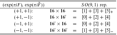
These four solutions represent just two physically distinct theories. In the IIA and IIA′ theories the R–R states have the opposite chirality on the left and the right, and in the IIB and IIB′ theories they have the same chirality. A spacetime reflection on a single axis, say

leaves the action and the constraints unchanged but reverses the sign of exp(πiF) in the left-moving R sectors and the sign of exp(πi) in the right-moving R sectors. At the massless level this switches the Weyl representations, 16 ↔ 16′. It therefore turns the IIA′ theory into IIA, and IIB′ into IIB.

Now suppose that there is no R–NS sector. By (c), there must be at least one R–R sector. In fact the combination of (NS+,NS+) with any single R–R sector solves (a), (b), and (c), but these turn out not to be modular-invariant. Proceeding further, one readily finds the only other solutions,

0A: (NS+,NS+) (NS−,NS−) (R+,R−) (R−,R+) ,

0B: (NS+,NS+) (NS−,NS−) (R+,R+) (R−,R−) .

These are modular-invariant, but both have a tachyon and there are no spacetime fermions.

In conclusion, we have found two potentially interesting string theories, the type IIA and IIB superstring theories. Referring back to table 10.3, one finds the massless spectra

The IIB theory is defined by keeping all sectors with

and the IIA theory by keeping all sectors with

This projection of the full spectrum down to eigenspaces of exp(πiF) and exp(πi) is known as the Gliozzi–Scherk–Olive (GSO) projection. In the IIA theory the opposite GSO projections are taken in the NS–R and R–NS sectors, so the spectrum is nonchiral. That is, the spectrum is invariant under spacetime parity, which interchanges 8 ↔ 8′ and 56 ↔ 56′. On the world-sheet, this symmetry is the product of spacetime parity and world-sheet parity. In the IIB theory the same GSO projection is taken in each sector and the spectrum is chiral.

The type 0 theories are formed by a different method: for example, 0B is defined by keeping all sectors with

The projections that define the type II theories act separately on the left-and right-moving spinors, while the projections that define the type 0 theory tie the two together. The latter are sometimes called diagonal GSO projections.

The most striking features of the type II theories are the massless vector–spinor gravitinos in the NS–R and R–NS sectors. The terminology type II refers to the fact that these theories each have two gravitinos. In the IIA theory the gravitinos have opposite chiralities (Γ eigenvalues), and in the IIB theory they have the same chirality. The NS–R gravitino state is

The physical state conditions are

as well as the equivalence relation

We have learned that such equivalence relations are the signature of a local spacetime symmetry. Here the symmetry parameter ζ_s is a spacetime spinor so we have local spacetime supersymmetry. In flat spacetime there will be a conserved spacetime supercharge , where A distinguishes the symmetries associated with the two gravitinos, and s is a spinor index of the same chirality as the corresponding gravitino. Thus the IIA theory has one supercharge transforming as the 16 of SO(9, 1) and one transforming as the 16′, and the IIB theory has two transforming as the 16.

The gravitino vertex operators are

The operators and , defined in eq. (10.4.25), have weights (1, 0) and (0, 1) and so are world-sheet currents associated with the spacetime supersymmetries.

This is our first encounter with spacetime supersymmetry, and the reader should now study the appropriate sections of appendix B. Section B.2 gives an introduction to spacetime supersymmetry. Section B.4 discusses antisymmetric tensor fields, which we have in the massless IIA and IIB spectra. Section B.5 briefly discusses the IIA and IIB supergravity theories which describe the low energy physics of the IIA and IIB superstrings. In each of the type II theories, there is a unique massless representation, which has 2⁸ = 256 states. The massless superstring spectra are the massless representations of IIA and IIB d = 10 spacetime supersymmetry respectively. This is to be expected: if all requirements for a consistent string theory are met (and they are) then the existence of the gravitinos implies that the corresponding supersymmetries must be present.

The reader may feel that the construction in this section, which is the Ramond–Neveu–Schwarz (RNS) form of the superstring, is somewhat adhoc. In particular one might expect that the spacetime supersymmetry should be manifest from the start. There is certainly truth to this, but the existing supersymmetric formulation (the Green–Schwarz superstring) seems to be even more unwieldy.

Note that the world-sheet and spacetime supersymmetries are distinct, and that the connection between them is indirect. The world-sheet supersymmetry parameter η(z) is a spacetime scalar and world-sheet spinor, while the spacetime supersymmetry parameter ζ_s is a spacetime spinor and world-sheet scalar. The world-sheet supersymmetry is a constraint in the world-sheet theory, annihilating physical states. The spacetime supersymmetry is a global symmetry of the world-sheet theory, giving relations between masses and amplitudes, though it becomes a local symmetry in spacetime.

Let us note one more feature of the GSO projection. In bosonized form, all the R sector vertex operators have odd length-squared and all the NS sector vertex operators have even length-squared, in terms of the ○ product defined in section 10.4. This can be seen at the lowest levels for the operators (10.4.22) and (10.4.25), the tachyon having been removed by the GSO projection. By the remark at the end of section 10.4, the space-time spin is then correlated with the world-sheet statistics. In fact, this is the same as the space-time statistics. The world-sheet statistics governs the behavior of the world-sheet amplitude under simultaneous exchange of world-sheet position, spacetime momentum, and other quantum numbers. After integrating over position, this determines the symmetry of the spacetime S-matrix. The result is the expected spacetime spin-statistics connection. Note that operators with the wrong spin-statistics connection, such as ψ^μ and e⁻, appear at intermediate stages but the projections that produce a consistent theory also give the spin-statistics connection. This is certainly a rather technical way for the spin-statistics theorem to arise, but it is worth noting that all string theories seem to obey the usual spin-statistics relation.

Unoriented and open superstrings

The IIB superstring, with the same chiralities on both sides, has a world-sheet parity symmetry Ω. We can gauge this symmetry to obtain an unoriented closed string theory.⁴ In the NS–NS sector, this eliminates the [2], leaving [0] + (2), just as it does in the unoriented bosonic theory. The fermionic NS–R and R–NS sectors of the IIB theory have the same spectra, so the Ω projection picks out the linear combination (NS–R) + (R–NS), with massless states 8′ + 56. In particular, one gravitino survives the projection. Finally, the existence of the gravitino means that there must be equal numbers of massless bosons and fermions, so a consistent definition of the world-sheet parity operator must select the [2] from the R–R sector to give 64 of each. One can understand this as follows. The R–R vertex operators

transform as 8 × 8 = [0] + [2] + [4]₊. The [0] and [4]₊ are symmetric under interchange of s and s′ and the [2] antisymmetric (one can see this by counting states, 36 versus 28, or in more detail by considering the S_a eigenvalues of the representations). World-sheet parity adds or subtracts a tilde to give

where the final sign comes from the fermionic nature of the R vertex operators. Thus, projecting onto Ω = +1 picks out the antisymmetric [2]. The result is the type I closed unoriented theory, with spectrum

However, this theory by itself is inconsistent, as we will explain further below.

Now consider open string theories. Closure of the OPE in open + open → closed scattering implies that any open string that couples consistently to type I or type II closed superstrings must have a GSO projection in the open string sector. The two possibilities and their massless spectra are

I: NS+, R+ = 8_v + 8 ,

: NS+, R− = 8_v + 8′ .

Adding Chan–Paton factors, the gauge group will again be U(n) in the oriented case and SO(n) or Sp(k) in the unoriented case. The 8 or 8′ spinors are known as gauginos because they are related to the gauge bosons by supersymmetry. They must be in the adjoint representation of the gauge group, like the gauge bosons, because supersymmetry commutes with the gauge symmetry.

We can already anticipate that not all of these theories will be consistent. The open string multiplets, with 16 states, are representations of d = 10, N = 1 supersymmetry but not of N = 2 supersymmetry. Thus the open superstring cannot couple to the oriented closed superstring theories, which have two gravitinos.⁵ It can only couple to the unoriented closed string theory (10.6.18) and so the open string theory must also be unoriented for consistent interactions. With the chirality (10.6.18), the massless open string states must be 8_v + 8. This is required by spacetime supersymmetry, or by conservation of exp(πiF) on the world-sheet. The result is the unoriented type I open plus closed superstring theory, with massless content

There is a further inconsistency in all but the SO(32) theory. We will see in section 10.8 that for all other groups, as well as the purely closed unoriented theory, there is a one-loop divergence and superconformal anomaly. We will also see, in chapter 12, that the spacetime gauge and coordinate symmetries have an anomaly at one loop for all but the SO(32) theory.

Thus we have found precisely three tachyon-free and nonanomalous string theories in this chapter: type IIA, type IIB, and type I SO(32).

10.7 Modular invariance

Superstring interactions are the subject of the next chapter, but there is one important amplitude that involves no interactions, only the string spectrum. This is the one-loop vacuum amplitude, studied for the bosonic string in chapter 7. We study the vacuum amplitude for the closed superstring in this section and for the open string in the next.

We make the guess, correctly it will turn out, that the torus amplitude is again given by the Coleman–Weinberg formula (7.3.24) with the region of integration replaced by the fundamental region for the moduli space of the torus:

with q = exp(2πiτ). We have included the minus sign for spacetime fermions from the Coleman–Weinberg formula, distinguishing the spacetime fermion number F from the world-sheet fermion number F. The masses are given in terms of the left- and right-moving parts of the transverse Hamiltonian by

The trace includes a sum over the different (α, F; ) sectors of the superstring Hilbert space. In each sector it breaks up into a product of independent sums over the transverse X, ψ, and oscillators, and the transverse Hamiltonian similarly breaks up into a sum. Each transverse X contributes as in the bosonic string, the total contribution of the oscillator sum and momentum integration being as in eq. (7.2.9),

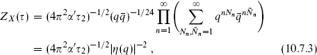
where 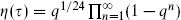. In addition there is a factor i(4π²α′τ₂)⁻¹ from the k^0,1 integrations.

For the ψs, the mode sum in each sector depends on the spatial periodicity α and includes a projection operator [1 ± exp(πiF)]. Although for the present we are interested only in R and NS periodicities, let us work out the partition functions for the more general periodicity (10.3.20),

where again α = 1 – 2ν. By the definition (10.3.23) of the ground state, the raising operators are

The ground state weight was found to be α²/8. Then

To define the general boundary conditions we have joined the fermions into complex pairs. Thus we can define a fermion number Q which is +1 for ψ and –1 for . To be precise, define Q to be the H-momentum in the bosonization (10.3.10) so that it is conserved by the OPE. The bosonization (10.3.25) then gives the charge of the ground state as α/2. Thus we can define the more general trace

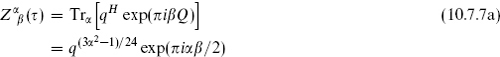
The notation in the final line was introduced in section 7.2, but our discussion of these functions in the present volume will be self-contained.

The charge Q modulo 2 is the fermion number F that appears in the GSO projection. Thus the traces that are relevant for the ten-dimensional superstring are

We should emphasize that these traces are for a pair of dimensions.

Tracing over all eight fermions, the GSO projection keeps states with exp(πiF) = +1. This is (τ), where

The half is from the projection operator, the minus sign in the second term is from the ghost contribution to exp(πiF), and the minus signs in the third and fourth (R sector) terms are from spacetime spin-statistics. For in the IIB theory one obtains the conjugate (τ)*. In the IIA theory, = − 1 in the R sector so the result is (τ)*. In all,

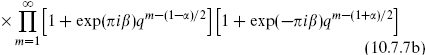
We know from the discussion of bosonic amplitudes that modular invariance is necessary for the consistency of string theory. In the superstring this works out in an interesting way. The combination is modular-invariant, as is Z_X. To understand the modular transformations of the fermionic traces, note that Z^α_β is given by a path integral on the torus over fermionic fields ψ with periodicities

This gives

Naively then, Z^α_β(τ) = Z^α_α+β−1(τ + 1), since both sides are given by the same path integral. Also, defining w′ = w/τ and ψ′(w′) = ψ(w),

so that naively Z^α_β(τ) = Z^β_−α(−1/τ). It is easy to see that by these two transformations one can always reach a path integral with α = 1, accounting for rule (c) from the previous section.

The reason these modular transformations are naive is that there is no diff-invariant way to define the phase of the path integral for purely left-moving fermions. For left- plus right-moving fermions with matching boundary conditions, the path integral can be defined by Pauli–Villars or other regulators. This is the same as the absolute square of the left-moving path integral, but leaves a potential phase ambiguity in that path integral separately.⁶ The naive result is correct for τ → − 1/τ, but under τ → τ + 1 there is an additional phase,

The τ → τ + 1 transformation follows from the explicit form (10.7.7b), the phase coming from the zero-point energy with the given boundary conditions. The absence of a phase in τ → −1/τ can be seen at once for τ = i. Note that Z¹₁ actually vanishes due to cancellation between the two R sector ground states, but we have assigned a formal transformation law for a reason to be explained below.

The phase represents a global gravitational anomaly, an inability to define the phase of the path integral such that it is invariant under large coordinate transformations. Of course, a single left-moving fermion has c ≠ and so has an anomaly even under infinitesimal coordinate transformations, but the global anomaly remains even when a left- and right-moving fermion are combined. For example, the product Z¹₀(τ)*Z⁰₀(τ) has no infinitesimal anomaly and should come back to itself under τ → τ + 2, but in fact picks up a phase exp(−πi/2). This phase arises from the level mismatch, the difference of zero-point energies in the NS and R sectors.

The reader can verify that with the transformations (10.7.14), the combinations are invariant under τ → − 1/τ and are multiplied by exp(2πi/3) under τ → τ + 1. Combined with the conjugates from the right-movers, the result is modular-invariant and the torus amplitude consistent. It is necessary for the construction of this invariant that there be a multiple of eight transverse fermions. Recall from section 7.2 that invariance under τ → τ + 1 requires that L₀ − ₀ be an integer for all states. For a single real fermion in the R–NS sector the difference in ground state energies is . For eight fermions this becomes , so that states with an odd number of NS excitations (as required by the GSO projection) are level-matched. Note also that modular invariance forces the minus signs in the combination (10.7.9), in particular the relative sign of (Z⁰₀)⁴ and (Z¹₀)⁴ which corresponds to Fermi statistics for the R sector states.

In the type 0 superstrings the fermionic trace is

with N = 8. This is known as the diagonal modular invariant, and it is invariant for any N because the phases cancel in the absolute values.

The type II theories have spacetime supersymmetry. This implies equal numbers of bosons and fermions at each mass level, and so Z_T2 should vanish in these theories by cancellation between bosons and fermions. Indeed it does, as a consequence of Z¹₁ = 0 and the ‘abstruse identity’ of Jacobi,

The same cancellation occurs in the open and unoriented theories.

Although we have focused on the path integral without vertex operators, amplitudes with vertex operators must also be modular-invariant. In the present case the essential issue is the path integral measure, and one can show by explicit calculation (or by indirect arguments) that the modular properties are the same with or without vertex operators. However, with a general vertex operator insertion the α = β = 1 path integral will no longer vanish, nor will the sum of the other three. The general amplitude will then be modular-invariant provided that the vacuum is modular-invariant without using the vanishing of Z¹₁ or the abstruse identity (10.7.16) — as we have required.

More on c = 1 CFT

The equality of the bosonic and fermionic partition functions (10.3.17) and (10.3.18) was one consequence of bosonization. These partition functions are not modular-invariant and so do not define a sensible string background. The fermionic spectrum consists of all NS–NS states. The bosonic spectrum consists of all states with integer k_R and k_L; this is not the spectrum of toroidal compactification at any radius. The simplest modular-invariant fermionic partition function is the diagonal invariant, taking common periodicities for the left- and right-movers. In terms of the states, this amounts to projecting

The NS–NS sector consists of the local operators we have been considering, and the chirality projection exp(πiF) = exp(πi) means that on the bosonic side k_R = k_L mod 2. The bosonic equivalents for the R–R sector states have half-integral k_R and k_L with again k_R = k_L mod 2. In all,

for integers n₁ and n₂ such that n₁ − n₂ ∈ 2Z This is the spectrum of a boson on a circle of radius 2, or 1 by T-duality, which we see is equivalent to a complex fermion with the diagonal modular-invariant projection. (The dimensionless radius r for the H scalar corresponds to the radius R = r(α′/2)^1/2 for X^µ, so r = 2^1/2 is self-dual.)

To obtain an equivalent fermionic theory at arbitrary radius, add

to the world-sheet Lagrangian density. The H theory is still free, but the equivalent fermionic theory is now an interacting field theory known as the Thirring model. The Thirring model has a nontrivial perturbation series but is solvable precisely because of its equivalence to a free boson. Actually, for any rational r, the bosonic theory is also equivalent to a free fermion theory with a more complicated twist (exercise 10.15).

Another interesting CFT consists of the set of vertex operators with

(This discussion should actually be read after section 11.1.) It is easy to check that this has the same properties as the set of vertex operators with integer k_R,L. That is, it is a single-valued operator algebra, but does not correspond to the spectrum of the string for any value of r, and does not have a modular-invariant partition function. Its special property is the existence of the operators

These have weights (, 0) and (0, ): they are world-sheet supercurrents! This CFT has (2,2) world-sheet supersymmetry. The standard representation, in which the supercurrent is quadratic in free fields, has two free X and two free ψ fields for central charge 3. This is rather more economical, with one free scalar and central charge 1. The reader can readily check that with appropriate normalization the supercurrents generate the N = 2 OPE (11.1.4).

This theory becomes modular-invariant if one twists by the symmetry

This projects the spectrum onto states with m − n ∈ 6Z and adds in a twisted sector with m, n ∈ Z + The resulting spectrum is the string theory at r = 2 × 3^1/2. This twist is a diagonal GSO projection, in that the supercurrent is odd under the symmetry.

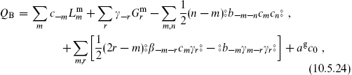
10.8 Divergences of type I theory

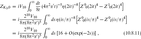
The cylinder, Möbius strip, and Klein bottle have no direct analog of the modular group, but the condition that the tadpole divergences cancel among these three graphs plays a similar role in restricting the possible consistent theories. The cancellation is very similar to what we have already seen in the bosonic theory in chapter 7. The main new issue is the inclusion of the various sectors in the fermionic path integral, and in particular the separate contributions of closed string NS–NS and R–R tadpoles.

The cylinder

Consider first the cylinder, shown in figure 10.1(a). One can immediately write down the amplitude by combining the bosonic result (7.4.1), converted to ten dimensions, with the fermionic trace (10.7.9) from one side of the type II string. We write it as a sum of two terms,

Fig. 10.1. (a) Cylinder in the limit of small t. (b) Analogous field theory graph.

where

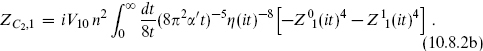
Note that the GSO and Ω projection operators each contribute a factor of . We have separated the terms according to whether exp(πiF) appears in the trace. In Z_C2,₀ it does not, and so the ψ^µ are antiperiodic in the σ² direction. In Z_C2,₁ it does appear and the ψ^µ are periodic. We can also regard the cylinder as a closed string appearing from and returning to the vacuum as in figure 10.1(b); we have used this idea in chapters 7 and 8. The periodicities of the ψ^µ mean that in terms of the closed string exchange, the part Z_C2,₀ comes from NS–NS strings and the part Z_C2,₁ from R–R strings.

We know from the previous section that the total fermionic partition function vanishes by supersymmetry, so that Z_C2,₁ = −Z_C2,₀; we concentrate then on Z_C2,₀. Using the modular transformations

and defining s = π/t, this becomes

The divergence as s → ∞ is due to a massless closed string tadpole, which as noted must be an NS–NS state. Thus we identify this as a dilaton plus graviton interaction (−G)^1/2e^−Φ coming from the disk, as in the bosonic string.

However, there is a paradox here: the d = 10, N = 1 supersymmetry algebra does not allow such a term. Even more puzzling, Z_C2,₁ has an equal and opposite divergence which must be from a tadpole of an R–R state, but the only massless R–R state is the rank 2 tensor which cannot have a Lorentz-invariant tadpole.

One can guess the resolution of this as follows. The type IIB string has rank n potentials for all even n, with n and 8 − n equivalent by Poincaré duality. The Ω projection removes n = 0 and its equivalent n = 8, as well as n = 4: all the multiples of four. This leaves n = 2, its equivalent n = 6 — and n = 10. A 10-form potential C₁₀ can exist in ten dimensions but its 11-form field strength dC₁₀ is identically zero. The integral of the potential over spacetime

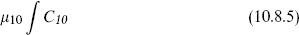
is invariant under δC₁₀ = d_χ9 and so can appear in the action. Since there is no kinetic term the propagator for this field is 1/0, and the effect of the tadpole is a divergence

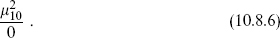
This must be the origin of the divergence in Z_C2,₁, as indeed a more detailed analysis does show. The equation of motion from varying C₁₀ is just µ₁₀ = 0, so unlike the divergences encountered previously this one cannot be removed by a correction to the background fields. It represents an actual inconsistency.

The Klein bottle

We know from the study of the bosonic string divergences that there is still the possibility of canceling this tadpole as shown in figure 10.2. The cylinder, Möbius strip, and Klein bottle each have divergences from the massless closed string states, the total being proportional to square of the sum of the disk and RP₂ tadpoles. The relative size of the two tadpoles depends on the Chan–Paton factors, and cancels for a particular gauge group.⁷

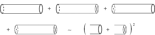
Fig. 10.2. Schematic illustration of cancellation of tadpoles.

The relation of the Möbius strip and Klein bottle as depicted in figure 10.2 to the twisted-strip and twisted-cylinder pictures was developed in section 7.4, and is shown in figure 10.3. In order to sum as in figure 10.2, one must rescale the surfaces so that the circumference in the σ² direction and length in the σ¹ directions are uniform; we have taken these to be 2π and s respectively. From figures 10.1 and 10.3 it follows that s is related to the usual modulus t for these surfaces by s = π/t, π/4t, and π/2t for the cylinder, Möbius strip, and Klein bottle respectively.

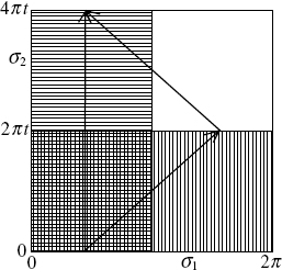
Fig. 10.3. Two fundamental regions for the Klein bottle. The right- and left-hand edges are periodically identified, as are the upper and lower edges. In addition the diagonal arrow shows an orientation-reversing identification. The vertically hatched region is a fundamental region for the twisted-cylinder picture, as is the horizontally hatched region for the decription with two crosscaps. As shown by the arrows, the periodicity of fields in the σ₂-direction of the latter description can be obtained by applying the orientation-reversing periodicity twice. The same picture applies to the Möbius strip, with the right- and left-hand edges boundaries, and with the range of σ₁ changed to π.

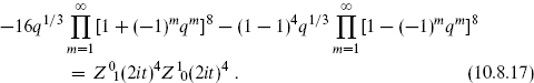
Each amplitude is obtained as a sum of traces, from summing over the various periodicity conditions and from expanding out the projection operators. We need to determine which terms contribute to the NS–NS exchange and which to the R–R exchange by examining the boundary conditions on the fermions in the world-sheet path integral. On the Klein bottle the GSO projection operator is

With R = Ωexp(πiβF + πi) in the trace, the path integral boundary conditions are

with the usual extra sign for fermionic fields. As indicated by the arrows in figure 10.3, these imply that

The NS–NS exchange, from the sectors antiperiodic under σ² → σ² + 4πt, then comes from traces weighted by Ωexp(πiF) or Ωexp(πi); further, these two traces are equal. Both NS–NS and R–R states contribute to the traces, making the separate contributions⁸

where q = exp(−2πt).

The full Klein bottle contribution to the NS–NS exchange is then

and Z_K2,₁ = −Z_K2,₀. The bosonic part is (7.4.15) converted to D = 10.

The Mobius strip

In the open string Ω acts as

using the doubling trick (10.2.15). In terms of the modes this is

The phase is imaginary in the NS sector and squares to −1. Thus

Since exp(πiF) = 1 by the GSO projection, this is physically the same as squaring to the identity, but the combined Ω and GSO projections require a single projection operator

With R = Ωexp(πiβF) in the trace, the fields have the periodicities

It follows that in the R sector of the trace the fields are periodic in the σ²-direction, corresponding to the R–R exchange, while the NS sector of the trace gives the NS–NS exchange.

It is slightly easier to focus on the R–R exchange, where the traces with Ω and Ωexp(πiF) sum to

The full Möbius amplitude, rewriting the bosonic part slightly, is

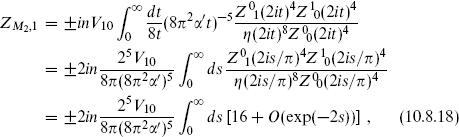
where the upper sign is for SO(n). We have used (7.4.22) in D = 10.

The total divergence from R–R exchange is

The R–R tadpole vanishes only for the gauge group SO(32). For each world-sheet topology the NS–NS divergence is the negative of the R–R divergence, so the dilaton–graviton tadpole also vanishes for SO(32). This calculation does not determine the sign of the tadpole, but it should be n 32. That is, changing from a symplectic to orthogonal projection changes the sign of RP₂, not of the disk. This is necessary for unitarity: the number of cross-caps is conserved mod 2 when a surface is cut open, so the sign is not determined by unitarity; this is not the case for the number of boundaries.

Exercises

10.1 (a) Find the OPE of T_F with X^µ and ψ^µ.

(b) Show that the residues of the OPEs of the currents (10.1.9) are proportional to the superconformal variations (10.1.10).

10.2 (a) Verify the commutator (10.1.11), up to terms proportional to the equations of motion.

(b) Verify that the commutator of a conformal and a superconformal transformation is a superconformal transformation.

10.3 (a) Verify the OPE (10.1.13).

(b) Extend this to the linear dilaton SCFT (10.1.22).

10.4 Obtain the R and NS algebras (10.2.11) from the OPE.

10.5 From the Jacobi identity for the R–NS algebra, show that the coefficients of the central charge terms in T_B T_B and T_FT_F are related.

10.6 Express exp(πiF) explicitly in terms of mode operators in the R and NS sectors of the ψ^µ CFT.

10.7 Verify that the expectation value (10.3.7) has the appropriate behavior as z_i → ∞, and show that together with the OPE this determines the result up to normalization.

10.8 Verify the weight of the fermionic ground state for general real ν :

(a) from the commutator (2.7.8);

(b) from the mnemonic of section 2.9.

The most direct, but most time-consuming, method would be to find the relation between conformal and creation–annihilation normal ordering as in eq. (2.7.11).

10.9 By any of the above methods, determine the ghost normal ordering constants (10.4.5).

10.10 Enumerate the states corresponding to each term in the expansion (10.3.19), in both fermionic and bosonic form.

10.11 Find the fermionic operator F_n equivalent to e^±inH(z). Here are two possible methods: build F_n iteratively in n by taking repeated operator products with e^±inH(z); or deduce . F_n directly from the OPE. Check your answer by comparing dimensions and fermion numbers.

10.12 By looking at the eigenvalues of S_a, verify the spinor decompositions (10.5.17).

10.13 (a) Verify the operator products (10.5.22).

(b) Using the Jacobi identity as in exercise 4.3, verify nilpotence of Q_B.

10.14 Work out the massless level of the open superstring in BRST quantization.

10.15 Consider a single complex fermion, with the spectrum summed over all sectors such that ν = is a multiple of 1/2p for integer p. Impose the projection that the numbers of left- and right-moving excitations differ by a multiple of 2p. Show that the spectrum is the same as that of a periodic scalar at radius r = 1/p. Show that this can be understood as a Z_p twist of the r = 1 theory. A further Z_2q twist of the T-dual r = 2p theory produces an arbitrary rational value.

¹ Lorentz invariance of the OPE holds separately for the ψ and X CFTs (and the CFT in the closed string) because they are decoupled from one another. However, the world-sheet supercurrent is only invariant under the overall Lorentz transformation.

² The precise operator definition has a subtlety when there are several species of fermion. The H^a for different a are independent and so the exponentials commute rather than anticommute. A cocycle is needed, as in eq. (8.2.22). A general expression will be given in the next section.

³ The bcβγ theory actually has a one-parameter family of superconformal symmetries, related by rescaling β → xβ and γ → x⁻¹γ. The general BRST construction (4.3.14) singles out the symmetry (10.1.21); this is most easily verified by noting that it correctly leads to the OPEs (10.5.22).

⁴ The analogous operation in the IIA theory would be to gauge the symmetry which is the product of world-sheet and spacetime parity, but this breaks some of the Poincaré invariance. We will encounter this in section 13.2.

⁵ At the world-sheet level the problem is that the total derivative null gravitino vertex operators give rise to nonzero world-sheet boundary terms. Only one linear combination of the two null gravitinos decouples, so we must make the world-sheet parity projection in order to eliminate the other.

⁶ The phase factor is a holomorphic function of τ, because the Z^α_β are. Since it has magnitude 1, this implies that it is actually independent of τ.

⁷ In the vacuum amplitude the sum of the NS–NS and R–R divergences is zero for each topology separately because the trace vanishes by supersymmetry. This is not sufficient, because they will no longer cancel when vertex operators are added near one end of each surface. The NS–NS and R–R tadpoles must vanish separately when summed over topologies.

⁸ In evaluating these, note that only states with identical ψ and excitations contribute to traces containing Ω. The signs from exp(πiF) or exp(πi) just cancel the signs from anticommuting ψs past s, so that all terms in each trace have the same sign. The overall sign in the NS–NS trace (positive) can be determined from the graviton, and the overall sign in the R–R trace (negative) from the argument (10.6.17).