11

The heterotic string

11.1 World-sheet supersymmetries

In the last chapter we were led by guesswork to the idea of enlarging the world-sheet constraint algebra, adding the supercurrents T_F(z) and Now let us see how much further we can generalize this idea. We are looking for sets of holomorphic and antiholomorphic currents whose Laurent coefficients form a closed algebra.

Let us start by emphasizing the distinction between global symmetries and constraints. Global symmetries on the world-sheet are just like global symmetries in spacetime, implying relations between masses and between amplitudes. However, we are also singling out part of the symmetry to impose as a constraint, meaning that physical states must be annihilated by it, either in the OCQ or BRST sense. In the bosonic string, the spacetime Poincaré invariance was a global symmetry of the world-sheet theory, while the conformal symmetry was a constraint. Our present interest is in constraint algebras. In fact we will find only a very small set of possibilities, but some of the additional algebras we encounter will appear later as global symmetries.

To begin we should note that the set of candidate world-sheet symmetry algebras is very large. In the bosonic string, for example, any product of factors ∂ⁿX^µ is a holomorphic current. In most cases the OPE of such currents will generate an infinite number of new currents, which is probably too big an algebra to be useful. However, even restricting to algebras with finite numbers of currents leaves an infinite number of possibilities.

Let us focus first on the holomorphic currents. We have seen in section 2.9 that in a unitary CFT an operator is holomorphic if and only if it is of weight (h, 0) with h ≥ 0. Although the complete world-sheet theory with ghosts and timelike oscillators does not have a positive norm, the spatial part does and so is a unitary representation of the symmetry. Because = 0, the spin of the current is also equal to h. Also, by taking real and imaginary parts we can assume the currents to be Hermitian. Now let us consider some possibilities:

Spin h ≥ 2. Algebras with spin > 2 currents are often referred to collectively as W algebras. Many are known, including several infinite families, but there is no complete classification. We will encounter one example in chapter 15, as a global symmetry of a CFT. There have been attempts to use some of these as constraint algebras. One complication is that the commutator of generators is in general a nonlinear function of the generators, making the construction of the BRST operator nontrivial. The few examples that have been constructed appear, upon gauge fixing, to be special cases of bosonic strings. Further, the geometric interpretation, analogous to the Riemann surface construction used to formulate bosonic string perturbation theory, is not clear. So we will restrict our attention to constraint algebras with h ≤ 2. Also, CFTs can have multiple (2, 0) currents as global symmetries. The bosonic string has at least 27, namely the ghost energy-momentum tensor and the energy-momentum tensor for each X^µ field. However, only the sum of these has a geometric interpretation, in terms of conformal invariance, and so we will assume that there is precisely one (2, 0) constraint current which is the overall energy-momentum tensor.

Spin h not a multiple of . For a current j of spin h,

with a coefficient that can be shown by a positivity argument not to vanish. This is multi-valued if 2h is not an integer. Although there are again many known CFTs with such currents, the nonlocality of these currents leads to substantial complications if one tries to impose them as constraints. Attempts to construct such fractional strings have led only to partial results and it is not clear if such theories exist. So we will restrict our attention to h a multiple of .

With these assumptions the possible algebras are very limited, with spins 0, , 1, , and 2. Solution of the Jacobi identities allows only the algebras shown in table 11.1. The first two entries are of course the conformal and N = 1 superconformal algebras that we have already studied. The three N = 4 algebras are related. The second algebra is a special case of the first where the U(1) current becomes the gradient of a scalar. The third is a subalgebra of the second.

Table 11.1. World-sheet superconformal algebras. The number of currents of each spin and the total ghost central charge are listed, as are the global symmetry generated by the spin-1 currents and the transformation of the supercharges under these.

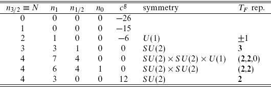
The ghost central charge is determined by the number of currents of each spin. The central charge for the ghosts associated with a current of spin h is

The sign (−1)^2h+1 takes into account the statistics of the ghosts, anticommuting for integer spin and commuting for half-integer spin. Since the matter central charge c^m is −c^g, there is only one new algebra, N = 2, that can have a positive critical dimension.

Actually, for N = 0 and N = 1 there can also be additional spin-1 and spin- constraints, provided the supercurrent is neutral under the corresponding symmetry. However, these larger algebras are not essentially different. The negative central charges of the ghosts allow additional matter, but the additional constraints precisely remove the added states so that these reduce to the old N = 0 and N = 1 theories. Nevertheless this construction is sometimes useful, as we will see in section 15.5.

For N = 2 it is convenient to join the two real supercurrents into one complex supercurrent

The N = 2 algebra in operator product form is then

In particular this implies that and j are primary fields and that has charge ±1 under the U(1) generated by j. The constant c in and jj must be the central charge. This follows from the Jacobi identity for the modes, but we will not write out the mode expansion in full until chapter 19, where we will have more need of it.

The smallest linear representation of the N = 2 algebra has two real scalars and two real fermions, which we join into a complex scalar Z and complex fermion ψ. The action is

The currents are

There is also a set of antiholomorphic currents, so this Zψ CFT has (2,2) superconformal symmetry.

The central charge of the Zψ CFT is 3, so two copies will cancel the ghost central charge. Since there are two real scalars in each CFT the critical dimension is 4. However, these dimensions come in complex pairs, so that the spacetime signature can be purely Euclidean, or (2, 2), but not the Minkowski (3, 1). Further, while the theory has four-dimensional translational invariance it does not have four-dimensional Lorentz invariance — the dimensions are paired together in a definite way in the supercharges. Instead the symmetry is U(2) or U(1, 1), complex rotations on the two Zs. Finally, the spectrum is quite small. The constraints fix two full sets Zψ oscillators (the analog of the light-cone gauge), leaving none. Thus there is just the center-of-mass motion of a single state. This has some mathematical interest, but whether it has physical applications is more conjectural.

Thus we have reduced what began as a rather large set of possible algebras down to the original N = 0 and N = 1. There is, however, another generalization, which is to have different algebras on the left- and rightmoving sides of the closed string. The holomorphic and antiholomorphic algebras commute and there is no reason that they should be the same. In the open string, the boundary conditions relate the holomorphic and antiholomorphic currents so there is no analogous construction.

This allows the one new possibility, the (N, Ñ) = (0, 1) heterotic string; (N, Ñ) = (1, 0) would be the same on redefining z → . We study this new algebra in detail in the remainder of the chapter. In addition the (0, 2) and (1, 2) heterotic string theories are mathematically interesting and may have a less direct physical relevance.

It should be emphasized that the analysis in this section had many explicit and implicit assumptions, and one should be cautious in assuming that all string theories have been found. Indeed, there are some string theories that do not fall into this classification. One is the Green-Schwarz form of the superstring. This has no simple covariant gauge-fixing, but in the light-cone gauge it is in fact equivalent to the RNS superstring, via bosonization. We will not have space to develop this in detail, but will see a hint of it in chapter 12. Another exception is topological string theory, where in a covariant gauge the constraints do not satisfy spin-statistics as we have assumed. This string theory has no physical degrees of freedom, but is of mathematical interest in that its observables are topological.

In fact, we will find the same set of physical string theories from an entirely different and nonperturbative point of view in chapter 14, suggesting that all have been found. To be precise, there are other theories with stringlike excitations, but the theories found in this and the previous chapter seem to be the only ones which have a limit where they become weakly coupled, so that a string perturbation theory exists.

11.2 The SO(32) and E₈ × E₈ heterotic strings

The (0, 1) heterotic string combines the constraints and ghosts from the left-moving side of the bosonic string with those from the right-moving side of the type II string. We could try to go further and combine the whole left-moving side of the bosonic string, with 26 flat dimensions, with the ten-dimensional right-moving side of the type II string. In fact this can be done, but since its physical meaning is not so clear we will for now keep the same number of dimensions on both sides. The maximum is then ten, from the superconformal side. We begin with the fields

with total central charge (c, ) = (10, 15). The ghost central charges add up to = (−26,−15), so the remaining matter has (c, ) = (16, 0). The simplest possibility is to take 32 left-moving spin- fields

The total matter action is

The operator products are

The matter energy-momentum tensor and supercurrent are

The world-sheet theory has symmetry SO(9, 1) × SO(32). The SO(32), acting on the λ^A, is an internal symmetry. In particular, none of the λ^A can have a timelike signature because there is no fermionic constraint on the left-moving side to remove states of negative norm. So while the action for the λ^A is the same as for the ^µ of the RNS superstring, the resulting theory is very different because of the constraints.

The right-moving ghosts are the same as in the RNS superstring, and the left-movers the same as in the bosonic string. It is straightforward to construct the nilpotent BRST charge and show the no-ghost theorem, with any BRST-invariant periodicity conditions. As usual this still holds if we replace any of the spatial (X^µ, ^µ) and the λ^A with a unitary (0,1) SCFT of the equivalent central charge.

To finish the description of the theory, we need to give the boundary conditions on the fields and specify which sectors are in the spectrum. This is more complicated than in the type II strings, because now neither Poincaré nor BRST invariance require common boundary conditions on all the λ^A. Periodicity of T_B only requires that the λ^A be periodic up to an arbitrary O(32) rotation,

We will not carry out a systematic search for consistent theories as we did for the RNS string, but will describe all the known theories. Nine tendimensional theories based on the action (11.2.3) are known, though six have tachyons and so are consistent only in the same sense as the bosonic string. Of the three tachyon-free theories, two have spacetime supersymmetry and these are our main interest. In this section we construct the two supersymmetric theories and in the next the seven nonsupersymmetric theories.

In the IIA and IIB superstrings the GSO projection acted separately on the left- and right-moving sides. This will be also true in any supersymmetric heterotic theory. The world-sheet current associated with spacetime symmetry is as in eq. (10.4.25), with s in the 16. In order for the corresponding charge to be well defined, the OPE of this current with any vertex operator must be single-valued. For the right-moving spinor part of the vertex operator, the spin eigenvalue s′ must then satisfy

for all s ∈ 16, where l is −1 in the NS sector and − in the R sector. Taking s = this condition is precisely the right-moving GSO projection

any other s ∈ 16 gives the same condition.

Now let us try a GSO projection on the left-moving spinors also. That is, we take periodicities

with the same sign on all 32 components, and impose

for the left-moving fermion number. It is easily verified by means of bosonization that the OPE is local and closed, just as in the IIA and IIB strings. Combine the 32 real fermions into 16 complex fermions,

These can then be bosonized in terms of 16 left-moving scalars H^K(z). By analogy to the definition of F in the type II string define

where λ^K± has q_K = ±1. Then F is additive so the OPE is closed, and the projection (11.2.10) guarantees that there are no branch cuts with the R sector vertex operators. Note that in the bosonized description we have 26 left-moving and 10 right-moving bosons, so the theory (11.2.3) really is a fusion (heterosis) of the bosonic and type II strings. We will emphasize the fermionic description in the present section, returning to the bosonic description later.

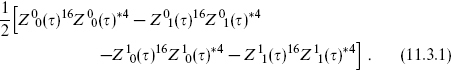
Modular invariance is straightforward. The partition function for the λ is

The modular transformations just permute the four terms, with no phase under τ → − 1/τ and a phase of exp(2πi/3) under τ → τ + 1. The latter cancels the opposite phase from the partition function (τ)* of . The form (11.2.13) parallels that of (τ) in the type II string but with all + signs. This is necessary from several points of view. With 32 rather than 8 fermions, the signs in the modular transformations are raised to the fourth power and so the first three terms must enter with a common sign. As usual the Z¹₁ term transforms only into itself and its sign depends on the chirality in the R sector. Three other theories, defined by flipping the chirality in one or both R sectors, are physically equivalent. Also, the relative minus sign in the first and second terms of (τ) came from the F of the superconformal ghosts, which we do not have on the left-moving side of the heterotic string. The relative minus sign in the first and third terms came from spacetime statistics, but the λ are spacetime scalars and so are their R sector states. So modular invariance, conservation of F by the OPE, and spacetime spin-statistics are all consistent with the partition function (11.2.13).

We now find the lightest states. The right-moving side is the same as in the type II string, with no tachyon and 8_v + 8 at the massless level. On the left-moving side, the normal ordering constant in the left-moving transverse Hamiltonian H^⊥ = α′m²/4 is

The left-moving NS ground state is therefore a tachyon. The first excited states

have H^⊥ = − but are removed by projection (11.2.10): the NS ground state now has exp(πiF) = +1 because there is no contribution from ghosts. A state of H^⊥ = 0 can be obtained in two ways:

The λ^A transform under an SO(32) internal symmetry. Under the full symmetry SO(8)_spin × SO(32), the NS ground state is invariant, (1, 1). The second state in (11.2.16) is antisymmetric under A ↔ B, so the massless states (11.2.16) transform as (8_v, 1) + (1, [2]). The antisymmetric tensor representation is the adjoint of SO(32), with dimension 32 × 31/2 = 496.

Table 11.2 summarizes the tachyonic and massless states on each side. The left-movers are given with their SO(8) × SO(32) quantum numbers and the right-movers with their SO(8) quantum numbers. Closed string states combine left- and right-moving states at the same mass. The leftmoving side, like the bosonic string, has a would-be tachyon, but there is no right-mover to pair it with so the theory is tachyon-free. At the massless level, the product

Table 11.2. Low-lying heterotic string states.

is the type I supergravity multiplet. The product

is an N = 1 gauge multiplet in the adjoint of SO(32). The latter is therefore a gauge symmetry in spacetime.

This is precisely the same massless content as the type I open plus closed SO(32) theory. However, these two theories have different massive spectra. In the open string, the gauge quantum numbers are carried by an SO(32) vector at each endpoint, so even at the massive levels there will never be more than a rank 2 tensor representation of the gauge group. In the heterotic string, the gauge quantum numbers are carried by fields that propagate on the whole world sheet. At massive levels any number of these can be excited, allowing arbitrarily large representations of the gauge group. Remarkably, however, we will see in chapter 14 that the type I and heterotic SO(32) theories are one and the same.

The second heterotic string theory is obtained by dividing the λ^A into two sets of 16 with independent boundary conditions,

with η and η′ each ±1. Correspondingly, there are the operators

which anticommute with λ^A for A = 1, …, 16 and A = 17, …, 32 respectively. Take separate GSO projections on the right-movers and the two sets of left-movers. That is, sum over the 2³ = 8 possible combinations of periodicities with the projections

Again closure and locality of the OPE and modular invariance are easily verified. In particular the partition function

transforms in the same way as and Z₁₆. It is important here that the fermions are in groups of 16, so that the minus signs from (which was for eight fermions) are squared.

As before, the lightest states on the right-hand side are the massless 8_v + 8. On the left-hand side, the sector NS–NS′ again has a normal ordering constant of −1, so the ground state is tachyonic but finds no matching state on the right. The first excited states, at m² = 0, are

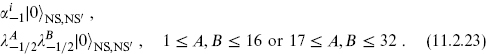
There is a difference here from the SO(32) case: because there are separate GSO projections on each set of 16, A and B must come from the same set. Since the SO(32) symmetry is partly broken by the boundary conditions, we classify states by the surviving SO(16) × SO(16). The states (11.2.23) include the antisymmetric tensor adjoint representation for each SO(16), with dimension 16 × 15/2 = 120.

In the left-moving R–NS′ sector the normal ordering constant is

so the ground states are massless. Making eight raising and eight lowering operators out of the 16 λ^A zero modes produces a 256-dimensional spinor representation of the first SO(16). The GSO projection separates it into two irreducible representations, 128 + 128′, the former being in the spectrum. The NS–R′ sector produces a 128 of the other SO(16), and the R–R′ sector again has no massless states.

In all, the SO(8) spin × SO(16) × SO(16) content of the massless level of the left-hand side is

Combining these with the right-moving 8_v gives, for each SO(16), massless vector bosons which transform as 120 + 128. Consistency of the spacetime theory requires that massless vectors transform under the adjoint representation of the gauge group. There is indeed a group, the exceptional group E₈, that has an SO(16) subgroup under which the E₈ adjoint 248 transforms as 120 + 128. Evidently this second heterotic string theory has gauge group E₈ × E₈. The world-sheet theory has a full E₈ × E₈ symmetry, even though only an SO(16) × SO(16) symmetry is manifest in the present description. The additional currents are given by bosonization as

This is a spin field, just as in the fermion vertex operator (10.4.25). For the first E₈ the charges are

and vice versa for the second. These are indeed (1, 0) operators. The massless spectrum is the d = 10, N = 1 supergravity multiplet plus an E₈ × E₈ gauge multiplet. The SO(8)_spin × E₈ × E₈ quantum numbers of the massless fields are

Consistency requires the fermions to be in groups of 16. We could make a modular-invariant theory using groups of eight, the left-moving partition function being ()⁴. However, we have seen that modular invariance requires minus signs in . These signs would give negative weight to left-moving R sector states and would correspond to the projection exp(πiF) = −1 in the NS sector. The first is inconsistent with spin-statistics because these states are spacetime scalars, and the second is inconsistent with closure of the OPE thus making the interactions inconsistent. The SO(32) and E₈ × E₈ theories are the only supersymmetric heterotic strings in ten dimensions.

11.3 Other ten-dimensional heterotic strings

The other heterotic string theories can all be constructed from a single theory by the twisting construction introduced in section 8.5. The ‘least twisted’ theory, in the sense of having the smallest number of path integral sectors, corresponds to the diagonal modular invariant

This invariant corresponds to taking all fermions, λ^A and ^µ, to be simultaneously periodic or antiperiodic on each cycle of the torus. In terms of the spectrum the world-sheet fermions are either all R or all NS, with the diagonal projection

This theory is consistent except for a tachyon, the state

which transforms as a vector under SO(32). At the massless level are the states

which are the graviton, dilaton, antisymmetric tensor and SO(32) gauge bosons. There are fermions in the spectrum, but the lightest are at m² = 4/α′.

Now let us twist by various symmetries. Consider first the Z₂ generated by exp(πi). Combined with the diagonal projection (11.3.2) this gives the total projection

This is the same as the projections (11.2.8) plus (11.2.10) defining the supersymmetric SO(32) heterotic string. Also, the spatial twist by exp(πi) adds in the sectors in which the λ^A and ^µ have opposite periodicities. The twisted theory is thus the SO(32) heterotic string. Twisting by exp(πiF) has the same effect.

Now consider twisting the diagonal theory by exp(πiF₁), which flips the sign of the first 16 λ^A and which was used to construct the E₈ × E₈ heterotic string. The resulting theory is nonsupersymmetric — as in eq. (11.2.8), a theory will be supersymmetric if and only if the projections include exp(πi) = 1. It has gauge group E₈ × SO(16) and a tachyon in the (1, 16). We leave it to the reader to verify this. A further twist by exp(πi) produces the supersymmetric E₈ × E₈ heterotic string.

One can carry this further by dividing the λ^A into groups of 8, 4, 2, and 1 as follows. Write the SO(32) index A in binary form, A = 1 + d₁d₂d₃d₄d₅, where each of the digits d_i is zero or one. Define the operators exp(πiF_i) for i = 1, …, 5 to anticommute with those λ^A having d_i = 0 and commute with those having d_i = 1. There are essentially five possible twist groups, with 2, 4, 8, 16, or 32 elements, generated respectively by choosing one, two, three, four or five of the exp(πiF_i) and forming all products. The first of these produces the E₈ × SO(16) theory just described; the further twists produce the gauge groups SO(24) × SO(8), E₇ × E₇ × SO(4), SU(16) × SO(2), and E₈. None of these theories is supersymmetric, and all have tachyons. A further twist by exp(πi) produces a supersymmetric theory which in each case is either the SO(32) theory or the E₈ × E₈ theory. These gauge symmetries are less manifest in this construction, with more of the currents coming from R sectors.

Let us review the logic of the twisting construction. The vertex operator corresponding to a sector twisted by a group element h produces branch cuts in the fields, but the projection onto h-invariant states means that these branch cuts do not appear in the products of vertex operators. Since h is a symmetry the projection is preserved by interactions. On the torus, the sum over spatial and timelike twists is modular-invariant, and this generalizes to any genus. However, we have learned in section 10.7 that naive modular invariance of the sum over path integral boundary conditions is not enough, because in general there are anomalous phases in the modular transformations. Only for a right–left symmetric path integral do the phases automatically cancel.

At one loop the anomalous phases appear only in the transformation τ → τ + 1, where they amount to a failure of the level-matching condition . It is further a theorem that for an Abelian twist group (like the products of Z₂s considered here), the one-loop amplitude and in fact all amplitudes are modular-invariant precisely if in every twisted sector, before imposing the projection, there is an infinite number of level-matched states. The projection can then be defined to satisfy level matching. In the heterotic string, taking a sector in which k of the λ^A satisfy R boundary conditions and 32−k satisfy NS boundary conditions, the zero-point energy is

The oscillators raise the energy by a multiple of , so the energies on the left-moving side are k mod . On the right-moving side we are still taking the fermions to have common boundary conditions for Lorentz invariance, so the energies are multiples of . Thus the level-matching condition is satisfied precisely if k is a multiple of eight. Closure of the OPE and spacetime spin-statistics actually require k to be a multiple of 16, as we have seen. The twists exp(πiF_i) were defined so that any product of them anticommutes with exactly 16 of the λ^A, satisfying this condition.

When the level-matching condition is satisfied, there can in fact be more than one modular-invariant and consistent theory. Consider a twisted theory with partition function

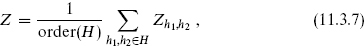
where h₁ and h₂ are the spatial and timelike periodicities on the torus. Then the theory with partition function

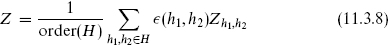
is also consistent (modular-invariant with closed and local OPE) provided that the phases (h₁, h₂) satisfy

In terms of ₂ defined in the original twisted theory, the new twisted theory is no longer projected onto H-invariant states, but onto states satisfying

in the sector twisted by h₁. In other words, states are now eigenvectors of , with a sector-dependent phase; equivalently we have made a sectordependent redefinition

The phase factor (h₁, h₂) is known as discrete torsion.

There is one interesting possibility for discrete torsion in the theories above, in the group generated by exp(πiF₁) and exp(πi) that produces the E₈ × E₈ string from the diagonal theory. For

the phase

satisfies the conditions (11.3.9). It modifies the projection from

which produces to the supersymmetric E₈ × E₈ string, to

The notation parallels that in eq. (10.7.11): under w → w+2π, the ^µ, the first 16 λ^A, and the second 16 λ^A pick up phases and respectively. The αs are conserved by the OPE so the projections are consistent. In other words, the spectrum consists of the sectors

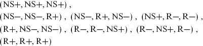
where the notation refers respectively to the ^µ, the first 16 λ^A, and the second 16 λ^A.

Gravitinos, in the sectors (R±, NS+, NS+), are absent from the spectrum. So also are tachyons, which are in the (NS−, NS−, NS+) and (NS−, NS+, NS−) sectors. The twists leave an SO(16) × SO(16) gauge symmetry. Classifying states by their SO(8)_spin × SO(16) × SO(16) quantum numbers, one finds the massless spectrum

This shows that a tachyon-free theory without supersymmetry is possible.

11.4 A little Lie algebra

In the open string the gauge charges are carried by the Chan–Paton degrees of freedom at the endpoints. In the closed string the charges are carried by fields that move along the string. We saw this earlier for the Kaluza–Klein gauge symmetry and the enhanced gauge symmetries that appear when the bosonic string is compactified, and now we see it again in the heterotic string. In the following sections we will discuss these closed string gauge symmetries in a somewhat more systematic way, but first we need to introduce a few ideas from Lie algebra. Space forbids a complete treatment; we focus on some basic ideas and some specific results that will be needed later.

Basic definitions

A Lie algebra is a vector space with an antisymmetric product [T, T′]. In terms of a basis T^a the product is

with f^ab_c the structure constants. The product is required to satisfy the Jacobi identity

The associated Lie group is generated by the exponentials

with the θ_a real. For a compact group, the associated compact Lie algebra has a positive inner product

which is invariant,

This invariance is equivalent to the statement that f^abc is completely antisymmetric, where d^ab is used to raise the index.

We are interested in simple Lie algebras, those having no nontrivial invariant subalgebras (ideals). A general compact algebra is a sum of simple algebras and U(1)s. For a simple algebra the inner product is unique up to normalization, and there is a basis of generators in which it is simply δ^ab. For any representation r of the Lie algebra (any set of matrices satisfying (11.4.1) with the given f^ab_c), the trace is invariant and so for a simple Lie algebra is proportional to d^ab,

from some constant T_r. Also, commutes with all the and so is proportional to the identity,

with Q_r the Casimir invariant of the representation r.

The classical Lie algebras are

• SU(n): Traceless Hermitean n × n matrices. The corresponding group consists of unitary matrices with unit determinant.¹ This algebra is also denoted A_n−1.

• SO(n): Antisymmetric Hermitean n×n matrices. The corresponding group SO(n, R) consists of real orthogonal matrices with unit determinant. For n = 2k this algebra is also denoted D_k. For n = 2k + 1 it is denoted B_k.

• Sp(k): Hermitean 2k × 2k matrices with the additional condition

Here the superscript T denotes the transpose, and

with I_k the k × k identity matrix. The corresponding group consists of unitary matrices U with the additional property

Confusingly, the notation Sp(2k) is also used for this group. It is also denoted C_k.

From each of the compact groups one obtains various noncompact groups by multiplying some generators by i. For example, the traceless imaginary matrices generate the group SL(n, R) of real matrices of unit determinant. The group SO(m, n, R) preserving a Lorentzian inner product is similarly obtained from SO(m+n). Another noncompact group is generated by imaginary rather than Hermitean matrices satisfying the symplectic condition (11.4.8) and consists of real matrices satisfying (11.4.10). This noncompact group is also denoted Sp(k) or Sp(2k); occasionally USp(2k) is used to distinguish the compact unitary case.

Such noncompact groups do not appear in Yang–Mills theory (the result would not be unitary) but they have other applications. Some of the SL(n, R) and SO(m, n, R) appear as low energy symmetries in compactified string theory, as discussed in section B.5 and chapter 14. The real form of Sp(k) is an invariance of the Poisson bracket in classical mechanics.

Roots and weights

A useful description of any Lie algebra h begins with a maximal set of commuting generators Hⁱ, i = 1, …, rank(g). The remaining generators E^α can be taken to have definite charge under the Hⁱ,

The rank(g)-dimensional vectors αⁱ are known as roots. It is a theorem that there is only one generator for a given root so the notation E^α is unambiguous. The Jacobi identity determines the rest of the algebra to be

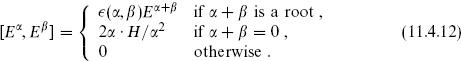
The products α·H and α² are defined by contraction with d_ij, the inverse of the inner product (11.4.4) restricted to the commuting subalgebra. Taking the trace with Hⁱ, the second equation determines the normalization (E^α, E^−α) = 2/α². The constants (α, β) take only the values ±1.

The matrices that represent Hⁱ can all be taken to be diagonal. Their simultaneous eigenvalues wⁱ, combined into vectors

are the weights, equal in number to the dimension of the representation. The roots are the same as the weights of the adjoint representation.

Examples:

• For SO(2k) = D_k, consider the k 2 × 2 blocks down the diagonal and let Hⁱ be

in the ith block and zero elsewhere. This is a maximal commuting set. The 2k-vectors (1, i, 0, …, 0) have eigenvalues

under the k Hⁱ; these are weights of the vector representation. The other weights are the same with the ±1 in any other position.

The adjoint representation is the antisymmetric tensor, which is contained in the product of two vector representations. The weights are additive so the roots are obtained by adding any distinct (because of the antisymmetry) pair of vector weights. This gives

and all permutations of these. The k zero roots obtained by adding any weight and its negative are just the Hⁱ.

The diagonal generators (11.4.14) are the same as are used in section B.1 to construct the spinor representations. In the spinor representation the weights wⁱ are given by all k-vectors with components ±, with the 2^k−1 having an even number of −s and the 2^k−1′ an odd number.

• For SO(2k+1) = B_k, one can take the same set of diagonal generators with a final row and a final column of zeros. The weights in the vector representation are the same as above plus (0^k) from the added row. The additional generators have roots

and all permutations.

• The adjoint of Sp(k) = C_k is the symmetric tensor, so one can obtain the roots as for SO(2k) except that the vector weights need not be distinct. The resulting roots are those of SO(2k) together with

and permutations. It is usually conventional to normalize the generators such that the longest root has length-squared two, so we must divide all the roots by 2^1/2.

• For SU(n) = A_n−1 it is useful first to consider U(n), even though this algebra is not simple. The n commuting generators H_i can be taken to have a 1 in the ii position and zeros elsewhere. The charged generator with a 1 in the ij position then has eigenvalue +1 under Hⁱ and −1 under H^j: the roots are all permutations of

Note that all roots lie in the hyperplane this is because all eigenvalues of the U(1) generator are zero. The roots of SU(n) are just the roots of U(n) regarded as lying in this hyperplane.

• We have stated that the E₈ generators decompose into the adjoint plus one spinor of SO(16). The commuting generators of SO(16) can also be taken as commuting generators of E₈, so the roots of E₈ are the roots of SO(16) plus the weights of the spinor, namely all permutations of the roots (11.4.16) plus

and the roots obtained from this by an even number of sign flips. Equivalently this set is described by

and

For A_n, D_k, and E₈ (and E₆ and E₇, which we have not yet described), all roots are of the same length. These are referred to as simply-laced algebras. For B_k and C_k (and F₄ and G₂) there are roots of two different lengths so one refers to long and short roots.

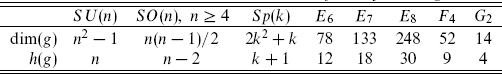
A quantity that will be useful later is the dual Coxeter number h(g) of the Lie algebra g, defined by

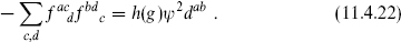
Here ψ is any long root. For reference, we give the values for all simple Lie algebras in table 11.3. The definition (11.4.22) makes h(g) independent of the arbitrary normalization of the inner product d^ab because the inverse appears in ψ² = ψⁱψ^jd_ij.

Useful facts for grand unification

The exceptional group E₈ is connected to the groups appearing in grand unification through a series of subgroups. This will play a role in the compactification of the heterotic string, and so we record without derivation the necessary results.

Table 11.3. Dimensions and Coxeter numbers for simple Lie algebras.

The first subgroup is

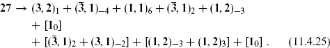
We have not described E₆ explicitly, but the reader can reproduce this and the decomposition (11.4.24) from the known properties of spinor representations, as well as the further decomposition of the E₆ representations in table 11.4 (exercise 11.5). In simple compactifications of the E₈ × E₈ string, the fermions of the Standard Model can all be thought of as arising from the 248-dimensional adjoint representation of one of the E₈s. It is therefore interesting to trace the fate of this representation under the successive symmetry breakings. Under E₈ → SU(3) × E₆,

That is, the adjoint of E₈ contains the adjoints of the subgroups, with half the remaining 162 generators transforming as a triplet of SU(3) and a complex 27-dimensional representation of E₆ and half as the conjugate of this. Further subgroups are shown in table 11.4. The first three subgroups correspond to successive breaking of E₆ down to the Standard Model group through smaller grand unified groups; the fourth is an alternate breaking pattern.

It is a familiar fact from grand unification that precisely one SU(3) × SU(2) × U(1) generation of quarks and leptons is contained in the 10 plus of SU(5). Tracing back further, we see that a generation fits into the single representation 16 of SO(10), together with an additional state 1₋₅. This extra state is neutral under SU(5), and so under SU(3) × SU(2) × U(1), and can be regarded as a right-handed neutrino. Going back to E₆ the 27 contains the 15 states of a single generation plus 12 additional states. Relative to SU(5) unification, SO(10) and E₆ are more unified in the sense that a generation is contained within a single representation, but less economical in that the representation contains additional unseen states as well. In fact, the latter may not be such a difficulty. To see why, consider the decomposition of the 27 of E₆ under SU(3) × SU(2) × U(1) ⊂ SU(5) ⊂ SO(10) ⊂ E₆:

Table 11.4. Subgroups and representations of grand unified groups.

        E₆ → SO(10) × U(1)

        78 → 45₀ + 16₋₃ + + 1₀

        27 → 1₄ + 10₋₂ + 16₁

SO(10) → SU(5) × U(1)

        45 → 24₀ + 10₄ + + 1₀

        16 → 10₋₁ + ₃ + 1₋₅

        10 → 5₂ + ₋₂

SU(5) → SU(3) × SU(2) × U(1)

        10 → (3, 2)₁ + (, 1)₋₄ + (1, 1)₆

         → (, 1)₂ + (1, 2)₋₃

E₆ → SU(3) × SU(3) × SU(3)

        78 → (8, 1, 1) + (1, 8, 1) + (1, 1, 8) + (3, 3, 3) + (, , )

        27 → (3, , 1) + (1, 3, ) + (, 1, 3)

The first line lists one generation, the second the extra state appearing in the 16 of SO(10), and the third the additional states in the 27 of E₆. The subset within each pair of square brackets is a real representation of SU(3) × SU(2) × U(1). The significance of this is that for a real representation r, the CPT conjugate also is in the representation r, and so the combined gauge plus SO(2) helicity representation for the particles plus their antiparticles is (r, +) + (r, − ). This is the same as for a massive spin- particle in representation r, so it is consistent with the gauge and spacetime symmetries for these particles to be massive. In the most general invariant action, all particles in [ ] brackets will have large (of order the unification scale) masses. It is notable that for any of the 10 + of SU(5), the 16 of SO(10), or the 27 of E₆, the natural SU(3) × SU(2) × U(1) spectrum is precisely a standard generation of quarks and leptons.

11.5 Current algebras

The gauge boson vertex operators in the heterotic string are of the form 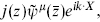where j(z) is either a fermion bilinear λ^Aλ^B or a spin field (11.2.26). Similarly the gauge boson vertex operators for the toroidally compactified bosonic string were of the form with j being ∂X^m for the Kaluza−Klein gauge bosons or an exponential for the enhanced gauge symmetry (or the same with right and left reversed). All these currents are holomorphic (1, 0) operators. In this section we consider general properties of such currents.

Let us consider in a general CFT the set of (1, 0) currents j^a(z). Conformal invariance requires their OPE to be of the form

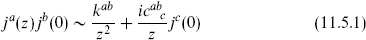
with k^ab and c^ab_c constants. Dimensionally, the z⁻² term must be a c-number and the z⁻¹ term must be proportional to a current. The Laurent coefficients

thus satisfy a closed algebra

In particular,

That is, the m = 0 modes form a Lie algebra g, and

We focus first on the case of simple g. The Jacobi identity requires that

This is the same relation as that defining the Lie algebra inner product d^ab, and since we are assuming g to be simple it must be that

for some constant . The algebra (11.5.3) is variously known as a current algebra, an affine Lie algebra, or an (affine) Kac−Moody algebra. The currents are (1, 0) tensors, so

Physically, the generate position-dependent g-transformations. This is possible in quantum field theory because there is a local current. The central extension or Schwinger term must always be positive in a unitary theory. To show this, note that

(no sum on a). For a compact Lie algebra d^aa is positive and so must be nonnegative. It can vanish only if = 0, but the vertex operator for is precisely the current j^a: any matrix element of j^a can be obtained by gluing into the world-sheet. Thus = 0 only if the current vanishes identically.

The coefficient is quantized. To show this, consider any root α. Defining

one finds from the general form (11.4.12) that these satisfy the SU(2) algebra

The reader can verify that the two sets

also satisfy the SU(2) algebra. The first is just the usual center-of-mass Lie algebra, while the second is known as pseudospin. From familiar properties of SU(2), 2J₃ must be an integer, and so 2/α² must be an integer. This condition is most stringent if α is taken to be one of the long roots of the algebra (denoted ψ). The level

is then a nonnegative integer, and positive for a nontrivial current.

It is common to normalize the Lie algebra inner product to give the long roots length-squared two, so that = k is the coefficient of the leading term in the OPE. We will usually do this in examples, as we have done in giving the roots of various Lie algebras in the previous section. Incidentally, it follows that with this normalization the generators (11.4.14) are normalized, so the SO(n) inner product is half of the vector representation trace. Similarly the inner product for SU(n) such that the long roots have length-squared two is equal to the trace in the fundamental representation. In general expressions we will keep the inner product arbitrary, inserting explicit factors of ψ² so that results are independent of the normalization. We will, however, take henceforth a basis for the generators such that d^ab = δ^ab

The level represents the relative magnitude of the z⁻² and z⁻¹ terms in the OPE. For U(1) the structure constant is zero and only the z⁻² term appears. Hence there is no analog of the level. It is convenient to normalize all the U(1) currents to

From this OPE and holomorphicity it follows that each U(1) current algebra is isomorphic to a free boson CFT,

We will often use this equivalence.

The current algebra in the heterotic string consisted of n real fermions λ^A(z). The currents

form an SO(n) algebra. The maximal set of commuting currents is iλ^2K−1λ^2K for K = 1, …, [n/2]. These correspond to the generators (11.4.14), which are normalized such that roots (11.4.16) have lengthsquared two. The level is then the coefficient of the leading term in the OPE; this is 1/z², so the level is k = 1. The case n = 3 is an exception: there are no long roots, only the short roots ±1, so we must rescale the diagonal current to 2^1/2iλ¹λ² and the level is k = 2.

For any real representation r of any Lie algebra, one can construct from dim(r) real fermions the currents

These satisfy a current algebra with level k = T_r/ψ², with T_r defined in eq. (11.4.6). The case in the previous paragraph is the n-dimensional vector representation of SO(n), for which T_R = ψ². As another example, nk fermions transforming as k copies of the vector representation give level k.

As a final example consider the SU(2) symmetry at the self-dual point of toroidal compactification. The current is exp[2^1/2iH(z)]. The current i∂H is then normalized so that the weight (from the OPE) is 2¹/², with length-squared two. The OPE of i∂H with itself starts as 1/z², so the level is again k = 1.

In some cases one may have sectors in which some currents are not periodic, j^a(w + 2π) = R^abj^b(w), where R^ab is any automorphism of the algebra. In these, the modes of the currents are fractional and satisfy a twisted affine Lie algebra.

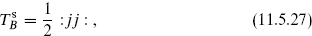
The Sugawara construction

In current algebras with conformal symmetry, there is a remarkable connection between the energy-momentum tensor and the currents, which leads to a great deal of interesting structure. Define the operator

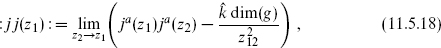
with the sum on a implicit. We first wish to show that up to normalization the OPE of : jj : with j^a is the same as that of T_B with j^a. This takes a bit of effort; the same calculation is organized in a different way in exercise 11.7.

The OPE of the product : jj : is not the same as the product of the OPEs, because the two currents in : jj : are closer to each other than they are to the third current; we must make a less direct argument using holomorphicity. Consider the following product:

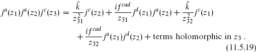
We have used the current−current OPE to determine the singularities as z₃ approaches z₁ or z₂, with a holomorphic remainder. In this relation take z₂ → z₁ and make a Laurent expansion in z₂₁, being careful to expand both the operator products and the explicit z₂ dependence. Keep the term of order (there is some cancellation from the antisymmetry of f^cad) to obtain

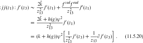
Here h(g) is again the dual Coxeter number. Define

The OPE of with the current is the same as that of the energy-momentum tensor T_B(z),

Now repeat the above with j^c(z₃) replaced by (z₃),

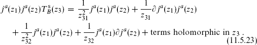
Again expand in z₂₁ and keep the term of order to obtain

with

This is of the standard form for an energy-momentum tensor, with central charge c^g,k. The Laurent coefficients

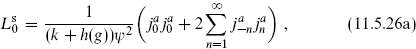
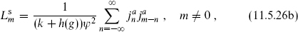
satisfy a Virasoro algebra with this central charge. The vanishing of the normal ordering constant in can be deduced by noting that holomorphicity requires and also for n ≥ 0 to annihilate the state |1.

We have used the jj OPE to determine the : jj :: jj : OPE. We could not do this directly, because the jj OPE is valid only for two operators close compared to all others, and in this case there are two additional currents in the vicinity. Naive application of the OPE would give the wrong normalization for T^s and c^g,k. The argument above uses the OPE only where it is valid, and then takes advantage of holomorphicity. The operator constructed from the product of two currents is known as a Sugawara energy-momentum tensor.

Finding the Sugawara tensor for a U(1) current algebra is easy. With the normalization (11.5.14) it is simply

as one sees by writing the current in terms of a free boson, j = i∂H.

The tensor may or may not be equal to the total T_B of the CFT. Define

Since the T_B and OPEs with j^a have the same singular terms, the product

is nonsingular. Since itself is constructed from the currents, this implies ∼ 0. Then

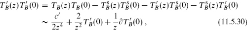
the standard TT OPE with central charge

The internal theory thus separates into two decoupled CFTs. One has an energy-momentum tensor constructed entirely from the current, and the other an energy-momentum tensor that commutes with the current. We will use the term current algebra to refer to the first factor alone, since the two CFTs are completely independent. For a unitary CFT c′ must be nonnegative and so

and is trivial precisely if

in which case T_B = .

We now consider examples. The dual Coxeter number can be written as a sum over the roots. For any simply-laced algebra, h(g) + 1 = dim(g)/rank(g), and so

For any simply-laced algebra at k = 1, the central charge is therefore

For the E₈×E₈ and SO(32) heterotic strings, this is the same as the central charge of the free fermion representation, and for the free boson representation of the next section: these are Sugawara theories. The operator : jj : looks as though it should be quartic in the fermions, but by using the OPE and the antisymmetry of the fermions one finds that reduces to the usual −λ^A∂λ^A.

Another example is SU(2) = SO(3), for which

We have seen the first CFT in this series (the self-dual point of toroidal compactification) and the second (free fermions). Most levels do not have a free-field representation. For any current algebra the central charge lies in the range

The first equality holds only for a simply-laced algebra at level one, and the second only for an Abelian algebra or in the limit k → ∞.

Primary fields

By acting repeatedly with the lowering operators with n > 0, one reaches a highest weight or primary state of the current algebra, a state annihilated by all the for n > 0. It is therefore also annihilated by the for n > 0, eq. (11.5.26), so is a highest weight state of the Virasoro algebra. The center-of-mass generators take primary states into primary states, so the latter form a representation of the algebra g,

with r (not summed) labeling the representation. It then follows that

with Q_r the Casimir (11.4.7). The weights of the primary fields are thus determined in terms of the algebra, level, and representation,

where Q_g is the Casimir for the adjoint representation. For SU(2) at level k, the weight of the spin-j primary is

It is also true that at any given level, only a finite number of representations are possible for the primary states. For any root α of g and any weight λ of r, the SU(2) algebra (11.5.12b) implies that

The left-hand side is and so ≥ − α · λ. Combining this with the same for −α gives

for all weights λ of r. Taking α to be a long root ψ, the level must satisfy

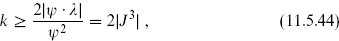
where J³ refers to the SU(2) algebra (11.5.12a) constructed from the charges and the root ψ. For g = SU(2) the statement is that the spin j of any primary state can be at most k. For example at k = 1, only the representations 1 and 2 are possible. For g = SU(3) at k = 1, only the 1, 3, and can appear. For g = SU(n) at level k, only representations whose Young tableau has k or fewer columns can appear.

The expectation values of primary fields are completely determined by symmetry. We defer the details to chapter 15.

Finally, let us briefly discuss the gauge symmetries of the type I theory in this same abstract language. The matter part of the gauge boson vertex operator is

on the boundary, where the λ^a are weight 0 fields. In a unitary CFT such λ^a must be constant by the equations of motion. The OPE is then

so the λ^a form a multiplicative algebra with structure constants d^ab_c. The antisymmetric part of d^ab_c is the structure constant of the gauge Lie algebra. This is an abstract description of the Chan−Paton factor. The requirement that the λ^a algebra be associative has been shown to forbid the gauge group E₈ × E₈.

11.6 The bosonic construction and toroidal compactification

We have seen in the construction of winding state vertex operators in section 8.2 that we may consider independent left- and right-moving scalars. Let us try to construct a heterotic string with 26 left-movers and 10 right-movers, which together with the ψ^µ give the correct central charge. The main issue is the spectrum of k_L,R; as in section 8.4 we use dimensionless momenta

in much of the discussion. Recall that an ordinary noncompact dimension corresponds to a left- plus a right-mover with taking continuous values; let there be d ≤ 10 noncompact dimensions. The remaining momenta,

take values in some lattice Γ. From the discussion of Narain compactification in section 8.4, we know that the requirements for a consistent CFT are locality of the OPE plus modular invariance. After taking the GSO projection on the right-movers, the conditions on Γ are precisely as in the bosonic case. Defining the product

the lattice must be an even self-dual Lorentzian lattice of signature (26 − d, 10 − d),

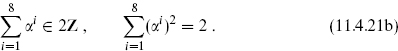
As in the bosonic case, where the signature was (26 − d, 26 − d), all such lattices have been classified. Consider first the maximum possible number of noncompact dimensions, d = 10. In this case, the ○ product has only positive signs, so the form an even self-dual Euclidean lattice of dimension 16. Even self-dual Euclidean lattices exist only when the dimension is a multiple of 8, and for dimension 16 there are exactly two such lattices, Γ₁₆ and Γ₈ × Γ₈. The lattice Γ₁₆ is the set of all points of the form

for any integers n_i. The lattice Γ₈ is similarly defined to be all points

The left-moving zero-point energy is −1 as in the bosonic string, so the massless states would have left-moving vertex operators ∂X^µ, ∂X^m, or e^ik_L·X(z) with = 2. Tensored with the usual right-moving 8_v + 8, the first gives the usual graviton, dilaton, and antisymmetric tensor. The 16 ∂X^m currents form a maximal commuting set corresponding to the m-momenta. The momenta are the charges under these and so are the roots of the gauge group. For Γ₁₆, the points of length-squared two are just the SO(32) roots (11.4.16). For Γ₈ the points of length-squared two are the E₈ roots (11.4.21). Thus the two possible lattices give the same two gauge groups, SO(32) and E₈ × E₈, found earlier. The commuting currents have singularity 1/z², so k = 1 again.

It is easy to see that the earlier fermionic construction and the present bosonic one are equivalent under bosonization. The integral points on the lattices (11.6.5) and (11.6.6) map to the NS sectors of the current algebra and the half-integral points to the R sectors. The constraint that the total be even is the GSO projection on the left-movers in each theory. We have seen in the previous section that the dynamics of a current algebra is completely determined by its symmetry, so we can give a representationindependent description of the left-movers as an SO(32) or E₈ × E₈ level one current algebra.²

Let us note some general results about Lie algebras and lattices. The set of all integer linear combinations of the roots of a Lie algebra g is known as the root lattice Γ_g of g. Now take any representation r and let λ be any weight of r. The set of points λ + v for all v ∈ Γ_g is denoted Γ_r. It can be shown by considering various SU(2) subgroups that for a simply-laced Lie algebra with roots of length-squared two,

The union of all Γ_r is the weight lattice Γ_w, and³

For example, the weight lattice of SO(2n) has four sublattices:

These are respectively the root lattice, the lattice containing the weights of the vector representation, and the lattices containing the weights of the two 2ⁿ⁻¹-dimensional spinor representations. The lattice Γ₈ is the root lattice of E₈ and is also the weight lattice because it is self-dual. The root lattice of SO(32) gives the integer points in Γ₁₆. The full Γ₁₆ is the root lattice plus one spinor lattice of SO(32).

The level one current algebra for any simply-laced Lie algebra g can similarly be represented by rank(g) left-moving bosons, the momentum lattice being the root lattice of g with the roots scaled to length-squared two. The constants (α, β) appearing in the Lie algebra (11.4.12) can then be determined from the vertex operator OPE; this is one situation where the explicit form of the cocycle is needed. A modular-invariant CFT can be obtained by taking also rank(g) right-moving bosons, with the momentum lattice being

That is, the spectrum runs over all sublattices of the weight lattice, with the left- and right-moving momenta taking values in the same sublattice.

Toroidal compactification

In parallel to the bosonic case, all even self-dual lattices of signature (26−d, 10−d) can be obtained from any single lattice by O(26−d, 10−d, R) transformations. Again start with any given solution Γ₀; for example, this could be either of the ten-dimensional theories with all compact dimensions orthogonal and at the SU(2) × SU(2) radius. Then any lattice

defines a consistent heterotic string theory. As in the bosonic case there is an equivalence

where

The moduli space is then

The discrete T-duality group O(26−d, 10−d, Z) of invariances of Γ₀ is understood to act on the right.

Now consider the unbroken gauge symmetry. There are 26 − d gauge bosons with vertex operators ∂x^mµ and 10 − d with vertex operators ∂x^mµ. These are the original 16 commuting symmetries of the tendimensional theory plus 10 − d Kaluza−Klein gauge bosons and 10 − d more from compactification of the antisymmetric tensor. In addition there are gauge bosons for every point on the lattice Γ such that

There are no gauge bosons from points with l_R ≠ 0 because the mass of such a state will be at least For generic boosts Λ, giving generic points in the moduli space, there are no points in Γ with l_R = 0 and so no additional gauge bosons; the gauge group is U(1)^36−2d. At special points the gauge symmetry is enhanced. Obviously one can get SO(32) × U(1)^20−2d or E₈ × E₈ × U(1)^20−2d from compactifying the original ten-dimensional theory on a torus without Wilson lines, just as in field theory. However, as in the bosonic string, there are stringy enhanced gauge symmetries at special points in moduli space. For example, the lattice Γ_{26−d,10−d}, defined by analogy to the lattices Γ₈ and Γ₁₆, gives rise to SO(52 − 2d) × U(1)^10−d. As in the bosonic case, the low energy physics near the point of enhanced symmetry is the Higgs mechanism. All groups obtained in this way have rank 36 − 2d. This is the maximum in perturbation theory, but we will see in chapter 19 that nonperturbative effects can lead to larger gauge symmetries.

The number of moduli, from the dimensions of the SO groups, is

As in the bosonic string these can be interpreted in terms of backgrounds for the fields of the ten-dimensional gauge theory. The compact components of the metric and antisymmetric tensor give a total of (10 − d)² moduli just as before. In addition there can be Wilson lines, constant backgrounds for the gauge fields A_m. As discussed in chapter 8, due to the potential Tr([A_m, A_n]²) the fields in different directions commute along flat directions and so can be chosen to lie in a U(1)¹⁶ subgroup. Thus there are 16(10 − d) parameters in A_m for (26 − d)(10 − d) in all.

In chapter 8 we studied quantization with antisymmetric tensor and open string Wilson line backgrounds. Here we leave the details to the exercises and quote the result. If we compactify x^m x^m + 2πR with constant backgrounds G_mn, B_mn, and then canonical quantization gives

where n_m and w^m are integers and q^I is on the Γ₁₆ or Γ₈ × Γ₈ lattice depending on which string has been compactified. The details are left to exercise 11.10. Let us note that with the gauge fields set to zero this reduces to the bosonic result (8.4.7). The terms in k_Lm and k_Rm that are linear in A^I come from the effect of the Wilson line on the periodicity, as in eq. (8.6.7). The term in that is linear in A^I comes about as follows. For a string that winds around the compact dimension, the Wilson line implies that the current algebra fermions are no longer periodic. The corresponding vertex operator (10.3.25) shows that the momentum is shifted. Finally, the terms quadratic in A^I can be most easily checked by verifying that α′k ○ k/2 is even.

To compare this spectrum with the Narain description one must go to coordinates in which G_m′n′ = δ_m′n′ so that the tetrad being defined by The discrete T-duality group is generated by T-dualities on the separate axes, large spacetime coordinate transformations, and quantized shifts of the antisymmetric tensor background and Wilson lines.

There is an interesting point here. Because the coset space (11.6.14) is the general solution to the consistency conditions, we must obtain this same set of theories whether we compactify the SO(32) theory or the E₈ × E₈ theory. From another point of view, note that the coset space is noncompact because of the Lorentzian signature — one can go to the limit of infinite Narain boost. Such a limit corresponds physically to taking one or more of the compact dimensions to infinite radius. Then one such limit gives the ten-dimensional SO(32) theory, while another gives the ten-dimensional E₈ × E₈ theory. Clearly one should think of all the different toroidally compactified heterotic strings as different states in a single theory. The two ten-dimensional theories are then distinct limits of this single theory.

Let us make the connection between these theories more explicit. Compactify the SO(32) theory on a circle of radius R, with G₉₉ = 1 and Wilson line

Adjoint states with one index from 1 ≤ A ≤ 16 and one from 17 ≤ A ≤ 32 are antiperiodic due to the Wilson line, so the gauge symmetry is reduced to SO(16) × SO(16). Now compactify the E₈×E₈ theory on a circle of radius R′ with G₉₉ = 1 and Wilson line

The integer-charged states from the SO(16) root lattice in each E₈ remain periodic while the half-integer charged states from the SO(16) spinor lattices become antiperiodic. Again the gauge symmetry is SO(16) × SO(16). To see the relation between these two theories, focus on the states that are neutral under SO(16) × SO(16), those with = 0. In both theories these are present only for w = 2m even, because of the shift in . The respective neutral spectra are

with the subscript 9 suppressed. The primes denote the E₈×E₈ theory, and = n + 2m, ′ = n′ + 2m′. We have used the explicit form of the Wilson line in each case, as well as the fact that = 0. Under (, m) ↔ (m′, ′) and , the spectra are identical if RR′ = α′/2. This symmetry extends to the full spectrum.

Finally let us ask how realistic a theory one obtains by compactification down to four dimensions. At generic points of moduli space the massless spectrum is given by dimensional reduction, simply classifying states by their four-dimensional symmetries. Analyzing the spectrum in terms of the four-dimensional SO(2) helicity, the SO(8) spins decompose as

and so

From the supergravity multiplet there is a graviton, with helicities ±2. There are four gravitinos, each with helicities ±. Toroidal compactification does not break any supersymmetry. Since in four dimensions the supercharge has four components, the 16 supersymmetries reduce to d = 4, N = 4 supersymmetry. The supergravity multiplet also includes 12 Kaluza−Klein and antisymmetric tensor gauge bosons, some fermions, and 36 moduli for the compactification. The final two spin-zero states are the dilaton and the axion. In four dimensions a two-tensor B_µν is equivalent to a scalar (section B.4). This is the axion, whose physics we will discuss further in chapter 18.

In ten dimensions the only fields carrying gauge charge are the gauge field and gaugino. These reduce as discussed in section B.6 to an N = 4 vector multiplet — a gauge field, four Weyl spinors, and six scalars, all in the adjoint. For enhanced gauge symmetries, which are not present in ten dimensions, one still obtains the same N = 4 vector multiplet because of the supersymmetry. Compactification with N = 4 supersymmetry cannot give rise to the Standard Model because the fermions are necessarily in the adjoint of the gauge group. One gravitino is good, as we will explain in more detail in section 16.2, but four are too much of a good thing. We will see in chapter 16 that a fairly simple orbifold twist reduces the supersymmetry to N = 1 and gives a realistic spectrum.

Supersymmetry and BPS states

A little thought shows that the supersymmetry algebra of the toroidally compactified theory must be of the form⁴

This differs from the simple dimensional reduction of the ten-dimensional algebra in that we have replaced P_m with P_Rm, the total right-moving momentum k_Rm of all strings in a given state. These are equal only for a state of total winding number zero. To obtain the algebra (11.6.23) directly from a string calculation requires some additional machinery that we will not develop until the next chapter. However, it is clear that the algebra must take this form because the spacetime supersymmetry involves only the right-moving side of the heterotic string.

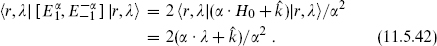
Let us look for Bogomolnyi−Prasad−Sommerfield (BPS) states, states that are annihilated by some of the Q_α. Take the expectation value of the algebra (11.6.23) in any state |ψof a single string of mass M in its rest frame. The left-hand side is a nonnegative matrix. The right-hand side is

The zero eigenvectors of this matrix are the supersymmetries that annihilate |ψ. Since (k_RmΓ^mΓ⁰)² = , the eigenvalues of the matrix (11.6.24) are

with half having each sign. A BPS state therefore has M² = . Recalling the heterotic string mass-shell conditions on the right-moving side,

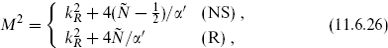
the BPS states are those for which the right-movers are in an R ground state or in an NS state with one ψ_−1/2 excited. The latter are the lowest NS states to survive the GSO projection, so it makes sense to change terminology at this point and call them ground states as well. The BPS states are then precisely those states for which the right-moving side is in its 8_v + 8 ground state, but with arbitrarily large k_R. These can be paired with many possible states on the left-moving side. The left-moving mass-shell condition is

or

Any left-moving oscillator state is possible, as long as the compact momenta and winding satisfy the condition (11.6.28). For any given leftmoving state, the 16 right-moving states 8_v + 8 form an ultrashort multiplet of the supersymmetry algebra, as compared to the 256 states in a normal massive multiplet.

It is interesting to look at the ten-dimensional origin of the modified supersymmetry algebra (11.6.23). Rewrite the algebra as

where X^m is the total winding of the string. Consider the limit that the compactification radii become macroscopic, so that a winding string is macroscopic as well. The central charge term in the supersymmetry algebra must be proportional to a conserved charge, so we are looking for a charge proportional to the length X of a string. Indeed, the string couples to the antisymmetric two-tensor field as

This is the natural generalization of the gauge coupling of a point particle, as discussed in section B.4. Integrating the current at fixed time gives the charge

the integral running along the world-line of the string. The full supersymmetry algebra is then

In ten noncompact dimensions the charge (11.6.31) vanishes for any finite closed string but can be carried by an infinite string, for example an infinite straight string which would arise as the R → ∞ limit of a winding string. It is often useful to contemplate such macroscopic strings, which of course have infinite total mass and charge but finite values per unit length. Under compactification the combination P_m − Q_m is the right-moving gauge charge. The left-moving charges do not appear in the supersymmetry algebra.

It is natural to wonder whether the algebra (11.6.32) is now complete, and in fact it is not. Consider compactification to four dimensions at a generic point in the moduli space where the gauge symmetry is broken to U(1)²⁸. Grand unified theories in which the U(1) of the Standard Model is embedded in a simple group always have magnetic monopoles arising from the quantization of topologically nontrivial classical solutions. String theory is not an ordinary grand unified theory but it also has magnetic monopoles. Compactification of the heterotic string leads to three kinds of gauge symmetry: the ten-dimensional symmetries, the Kaluza–Klein symmetries, and the antisymmetric tensor symmetries. For each there is a corresponding monopole solution: the ’t Hooft–Polyakov monopole, the Kaluza–Klein monopole, and the H-monopole respectively. Of course since the various charges are interchanged by the O(22, 6, Z) T-duality, the monopoles must be as well. Monopole charges appear in the supersymmetry algebra; in the present case it is again the right-moving charges that appear. In the low energy supergravity theory there is a symmetry that interchanges the electric and magnetic charges, so they must appear in the supersymmetry algebra in a symmetric way. We will discuss similar central charge terms extensively in chapters 13 and 14.

Exercises

11.1 Show that the operators (10.7.21) with appropriate normalization generate the full N = 2 superconformal algebra (11.1.4).

11.2 Show that if a (, 0) constraint is not tensor, then is a nonvanishing (, 0) constraint, and a linear combination of and is a tensor (, 0) constraint.

11.3 Show that if we take the GSO projection on the λ^A in groups of eight, modular invariance is inconsistent with spacetime spin-statistics. Show that the OPE does not close.

11.4 (a) Find the massless and tachyonic states in the theory obtained by twisting the diagonal theory on the group generated by exp().

(b) Do the same for the group generated by exp() and exp().

11.5 (a) The decompositions of the spinor representation under SO(16) → SO(6) × SO(10) and under SO(6) → SU(3) × U(1) are obtained in section B.1. Use this to show that the adjoint of decomposes into SU(3) representations with the degeneracies (11.4.24). The 78 generators neutral under SU(3) must form a closed algebra: this is E₆.

(b) Use the same decompositions to show that the E₆ representations decompose as shown in table 11.4 under E₆ → SO(10) × U(1).

(c) In a similar way obtain the decompositions shown in table 11.4 for SO(10) → SU(5) × U(1).

11.6 Repeat parts (a) and (b) of the previous exercise for SO(16) → SO(4) × SO(12) and SO(4) → SU(2) × U(1) to obtain the analogous properties of E₇.

11.7 Show that :jj(0) : = . Act with the Laurent expansion (11.5.2) for j^c(z) and verify the OPE (11.5.20) in the Sugawara construction. Similarly verify the OPE (11.5.24).

11.8 For the free-fermion currents (11.5.16) for SO(n), verify that the Sugawara construction gives the usual bilinear T_B.

11.9 Show that the lattice

is even and self-dual, where is a weight sublattice of SO(22), the same weight sublattice for SO(6), and the sum runs over the four sublattices of SO(2n). Show that this gives a four-dimensional compactification of the heterotic string with SO(44) × U(1)⁶ gauge symmetry.

11.10 (a) Verify the spectrum (11.6.17) for one compact dimension with a Wilson line background only.

(b) For the full spectrum (11.6.17), verify that is even for any state and that is integral for any pair of states. The ∘ product is

(c) (Optional) Verify the full result (11.6.17) by canonical quantization. Recall that the antisymmetric tensor background has already been treated in chapter 8. Reference: Narain, Sarmadi, & Witten (1987).

11.11 In the E₈ × E₈ string, the currents i∂H^I plus the vertex operators for the points of length two form a set of (1,0) currents satisfying the E₈ × E₈ algebra. From the 1/z term in the OPE, find the commutation relations of E₈. Be sure to include the cocycle in the vertex operator.

11.12 Find the Hagedorn temperatures of the type I, II, and heterotic string theories. Use the result (7.2.30) for the asymptotics of the partition function to express the Hagedorn temperature in general form.

¹ To be precise the Lie algebra determines only the local structure of the group. Many groups, differing only by discrete identifications, will have a common Lie algebra.

² To be precise it is still necessary to specify the spectrum, which amounts to specifying which primary fields appear. Modular invariance generally restricts the possibilities greatly.

³ For the nonsimply-laced algebras Sp(k) and SO(2k + 1), these same relations hold between the weight lattice of one and the dual of the root lattice of the other.

⁴ For clarity a projection operator is omitted — all spinor indices in this equation must be in the 16.