15

Advanced CFT

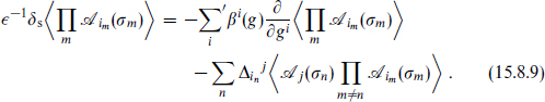
We have encountered a number of infinite-dimensional symmetry algebras on the world-sheet: conformal, superconformal, and current. While we have used these symmetries as needed to obtain specific physical results, in the present chapter we would like to take maximum advantage of them in determining the form of the world-sheet theory. An obvious goal, not yet reached, would be to construct the general conformal or superconformal field theory, corresponding to the general classical string background.

This subject is no longer as central as it once appeared to be, as spacetime rather than world-sheet symmetries have been the principal tools in recent times. However, it is a subject of some beauty in its own right, with various applications to string compactification and also to other areas of physics.

We first discuss the representations of the conformal algebra, and the constraints imposed by conformal invariance on correlation functions. We then study some examples, such as the minimal models, Sugawara and coset theories, where the symmetries do in fact determine the theory completely. We briefly summarize the representation theory of the N = 1 superconformal algebra. We then discuss a framework, rational conformal field theory, which incorporates all these CFTs. To conclude this chapter we present some important results about the relation between conformal field theories and nearby two-dimensional field theories that are not conformally invariant, and the application of CFT in statistical mechanics.

15.1 Representations of the Virasoro algebra

In section 3.7 we discussed the connection between classical string backgrounds and general CFTs. In particular, we observed that CFTs corresponding to compactification of the spatial dimensions are unitary and their spectra are discrete and bounded below. These additional conditions strongly restrict the world-sheet theory, and we will assume them throughout this chapter except for occasional asides.

Because the spectrum is bounded below, acting repeatedly with Virasoro lowering operators always produces a highest weight (primary) state |h, with properties

Starting from a highest weight state, we can form a representation of the Virasoro algebra

by taking |h together with all the states obtained by acting on |h with the Virasoro raising operators,

We will denote this state |h, {k} or L_−{k}|h for short. The state (15.1.3) is known as a descendant of h, or a secondary. A primary together with all of its descendants is also known as a conformal family. The integers {k} may be put in the standard order k₁ ≥ k₂ ≥ … ≥ k₁ ≥ 1 by commuting the generators. This process terminates in a finite number of steps, because each nonzero commutator reduces the number of generators by one. To see that this is a representation, consider acting on |h, {k} with any Virasoro generator L_n. For n < 0, commute L_n into its standard order; for n ≥ 0, commute it to the right until it annihilates |h. In either case, the nonzero commutators are again of the form |h, {k′}. All coefficients are determined entirely in terms of the central charge c from the algebra and the weight h obtained when L₀ acts on |h; these two parameters completely define the highest weight representation.

It is a useful fact that for unitary CFTs all states lie in highest weight representations — not only can we always get from any state to a primary with lowering operators, but we can always get back again with raising operators. Suppose there were a state | that could not be expanded in terms of primaries and secondaries. Consider the lowest-dimension state with this property. By taking

with |i running over a complete orthonormal set of primaries and secondaries, we may assume | to be orthogonal to all primaries and secondaries. Now, | is not primary, so there is a nonzero state L_n| for some n > 0. Since the CFT is unitary this has a positive norm,

The state L_n| lies in a highest weight representation, since by assumption | is the lowest state that does not, and so therefore does L_−nL_n|. Therefore it must be orthogonal to |, in contradiction to eq. (15.1.5).

This need not hold in more general circumstances. Consider the operator ∂X of the linear dilaton theory. Lowering this gives the unit operator, L₁ · ∂X = −α′V · 1, but L₋₁ · 1 = 0 so we cannot raise this operator back to ∂X. The problem is the noncompactness of X combined with the position dependence of the dilaton, so that even |1 is not normalizable.

Now we would like to know what values of c and h are allowed in a unitary theory. The basic method was employed in section 2.9, using the Virasoro algebra to compute the inner product

implying h ≥ 0. Consideration of another inner product gave c ≥ 0. Now look more systematically, level by level. At the second level of the highest weight representation, the two states L₋₁L₋₁|h and L₋₂|h have the matrix of inner products

Commuting the lowering operators to the right gives

and

In a unitary theory the matrix of inner products, and in particular its determinant, cannot be negative. The determinant is nonnegative in the region c ≥ 1, h ≥ 0, but for 0 < c < 1 a new region h₋ < h < h₊ is excluded.

At level N, the matrix of inner products is

Its determinant has been found,

with K_N a positive constant. This is the Kac determinant. The zeros of the determinant are at

where

The multiplicity P(N – rs) of each root is the partition of N – rs, the number of ways that N – rs can be written as a sum of positive integers (with P(0) ≡ 1):

At level 2, for example, the roots are h_1,1 = 0, h_2,1 = h₊, and h_1,2 = h_–, each with multiplicity 1, as found above.

The calculation of the determinant (15.1.11) is too lengthy to repeat here. The basic strategy is to construct all of the null states, those corresponding to the zeros of the determinant, either by direct combinatoric means or using some tricks from CFT. The determinant is a polynomial in h and so is completely determined by its zeros, up to a normalization which can be obtained by looking at the h → ∞ limit. The order of the polynomial is readily determined from the Virasoro algebra, so one can know when one has all the null states. Let us note one particular feature. At level 2, the null state corresponding to h_1,1 is L_–1L_–1|h = 0. This is a descendant of the level 1 null state L_–1|h = 0. In general, the zero h_r,s appears first at level rs. At every higher level N are further null states obtained by acting with raising operators on the level rs state; the partition P(N – rs) in the Kac determinant is the total number of ways to act with raising operators of total level N – rs.

A careful study of the determinant and its functional dependence on c and h shows (the analysis is again too lengthy to repeat here) that unitary representations are allowed only in the region c ≥ 1, h ≥ 0 and at a discrete set of points (c, h) in the region 0 ≤ c < 1:

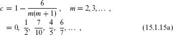
where 1 ≤ r ≤ m – 1 and 1 ≤ s ≤ m. The discrete representations are of great interest, and we will return to them in section 15.3.

For a unitary representation, the Kac determinant also determines whether the states |h, {k} are linearly independent. If it is positive, they are; if it vanishes, some linear combination(s) are orthogonal to all states and so by unitarity must vanish. The representation is then said to be degenerate. Of the unitary representations, all the discrete representations (15.1.15) are degenerate, as are the representations c = 1, h = n², n ∈ Z and c > 1, h = 0. For example, at h = 0 we always have L_–1 · 1 = 0, but at the next level L_–2 · 1 = T_zz is nonzero.

Let us make a few remarks about the nonunitary case. In the full matter CFT of string theory, the states L_–{k}|h obtained from any primary state |h are linearly independent when the momentum is nonzero. This can be seen by using the same light-cone decomposition used in the no-ghost proof of chapter 4. The term in L_–n of greatest N^lc is k^–. These manifestly generate independent states; the upper triangular structure then guarantees that this independence holds also for the full Virasoro generators.

A representation of the Virasoro algebra with all of the L_–{k}|h linearly independent is known as a Verma module. Verma modules exist at all values of c and h. Verma modules are particularly interesting when the dimension h takes a value h_r,s such that the Kac determinant vanishes. The module then contains nonvanishing null states (states that are orthogonal to all states in the module). Acting on a null state with a Virasoro generator gives a null state again, since for any null |ν and for any state |ψ in the module we have ψ|(L_n|ν) = (ψ|L_n)|ν = 0. The representation is thus reducible: the subspace of null states is left invariant by the Virasoro algebra.¹ The L_n for n > 0 must therefore annihilate the lowest null state, so this state is in fact primary, in addition to being a level rs descendant of the original primary state |h_r,s. That is, the h_r,s Verma module contains an h = h_r,s + rs Verma submodule. In some cases, including the special discrete values of c (15.1.15), there is an intricate pattern of nested submodules.

Clearly a Verma module can be unitary only at those values of c and h where nondegenerate unitary representations are allowed. At the (c, h) values with degenerate unitary representations, the unitary representation is obtained from the corresponding Verma module by modding out the null states.

As a final example consider the matter sector of string theory, c = 26. From the OCQ, we know that there are many null physical states at h = 1. This can be seen from the Kac formula as well. For c = 26, α₊ = 3i/6^1/2, α_– = 2i/6^1/2, and so

The corresponding null physical state is at

Any pair of positive integers with |3r – 2s| = 1 leads to a null physical state at h = 1. For example, the states (r, s) = (1, 1) and (1, 2) were constructed in exercise 4.2. With care, one can show that the number of null states implied by the Kac formula is exactly that required by the no-ghost theorem.

15.2 The conformal bootstrap

We now study the constraints imposed by conformal invariance on correlation functions on the sphere. In chapter 6 we saw that the Möbius subgroup, with three complex parameters, reduced the n-point function to a function of n – 3 complex variables. The rest of the conformal symmetry gives further information: it determines all the correlation functions of descendant fields in terms of those of the primary fields.

To begin, consider the correlation function of the energy momentum tensor T(z) with n primary fields . The singularities of the correlation function as a function of z are known from the T OPE. In addition, it must fall as z^–4 for z → ∞, since in the coordinate patch u = 1/z, T_uu = z⁴T_zz is holomorphic at u = 0. This determines the correlation function to be

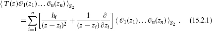
A possible holomorphic addition is forbidden by the boundary condition at infinity. In addition, the asymptotics of order z^–1, z^–2, and z^–3 must vanish; these are the same as the conditions from Möbius invariance, developed in section 6.7. The correlation function with several Ts is of the same form, with additional singularities from the TT OPE. Now make a Laurent expansion in z – z₁,

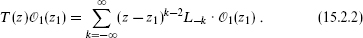
Then for k ≥ 1, matching coefficients of (z – z₁)^{k – 2} on the right and left of the correlator (expectation value) (15.2.1) gives

where

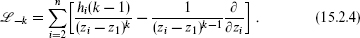
This extends to multiple generators, and to the antiholomorphic side,

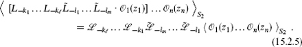
The additional terms from the TT OPE do not contribute when all the k_i and l_i are positive. The correlator of one descendant and n – 1 primaries is thus expressed in terms of that of n primaries. Clearly this can be extended to n descendants, though the result is more complicated because there are additional terms from the TT singularities.

Earlier we argued that the operator product coefficients were the basic data in CFT, determining all the other correlations via factorization. We see now that it is only the operator product coefficients of primaries that are necessary. It is worth developing this somewhat further for the four-point correlation. Start with the operator product of two primaries, with the sum over operators now broken up into a sum over conformal families i and a sum within each family,

where N is the total level of {k}. Writing the operator product coefficient c^{i{k, }}_mn as a three-point correlator and using the result (15.2.5) to relate this to the correlator of three primaries gives

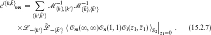
To relate the operator product coefficient to a correlator we have to raise an index, so the inverse ^–1 appears (with an appropriate adjustment for degenerate representations). The right-hand side is equal to the operator product of the primaries times a function of the coordinates and their derivatives, the latter being completely determined by the conformal invariance. Carrying out the differentiations in _–{k′} and _–{′} and then summing leaves

The coefficient is a function of the weights h_m, h_n, and h_i and the central charge c, but is otherwise independent of the CFT.

Now use the OPE (15.2.6) to relate the four-point correlation to the product of three-point correlations,

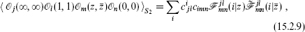
where

This function is known as the conformal block, and is holomorphic except at z = 0, 1, and ∞. The steps leading to the decomposition (15.2.9) show that the conformal block is determined by the conformal invariance as a function of h_j, h_l, h_m, h_n, h_i, c, and z. One can calculate it order by order in z by working through the definition.

Recall that the single condition for a set of operator product coefficients to define a consistent CFT on the sphere is duality of the four-point function, the equality of the decompositions (15.2.9) in the (jl)(mn), (jm)(ln), and (jn)(lm) channels. The program of solving this constraint is known as the conformal bootstrap. The general solution is not known. One limitation is that the conformal blocks are not known in closed form except for special values of c and h.

Beyond the sphere, there are the additional constraints of modular invariance of the zero-point and one-point functions on the torus. Here we will discuss only a few of the most general consequences. Separating the sum over states in the partition function into a sum over conformal families and a sum within each family yields

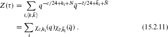
Here

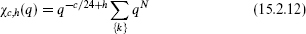
is the character of the (c, h) representation of the Virasoro algebra. For a Verma module the states generated by the L_–k are in one-to-one correspondence with the excitations of a free boson, generated by α_–k. Thus,

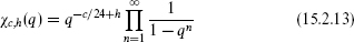
for a nondegenerate representation. For degenerate representations it is necessary to correct this expression for overcounting. A generic degenerate representation would have only one null primary, say at level N; the representation obtained by modding out the resulting null Verma module would then have character (1 – q^N)q^1/24η(q)^–1. For the unitary degenerate representations (15.1.15), with their nested submodules, the calculation of the character is more complicated.

In section 7.2 we found the asymptotic behavior of the partition function for a general CFT,

letting c = . For a single conformal family, letting q = exp(–2π),

Then for a general CFT

as → 0, with the total number of primary fields in the sum (15.2.11). Comparing this bound with the known asymptotic behavior (15.2.14), can be finite only if c < 1. So, while we have been able to use conformal invariance to reduce sums over states to sums over primaries only, this remains an infinite sum whenever c ≥ 1. The c < 1 theories, to be considered in the next section, stand out as particularly simple.

15.3 Minimal models

For fields in degenerate representations, conformal invariance imposes additional strong constraints on the correlation functions. Throughout this section we take c ≤ 1, because only in this range do degenerate representations of positive h exist. We will not initially assume the CFT to be unitary, but the special unitary values of c will eventually appear.

Consider, as an example, a primary field _1,2 with weight

For now we leave the right-moving weight unspecified. The vanishing descendant is

Inserting this into a correlation with other primary fields and using the relation (15.2.5) expressing correlations of descendants in terms of those of primaries gives a partial differential equation for the correlations of the degenerate primary,

where

For n = 4, the correlation is known from conformal invariance up to a function of a single complex variable, and eq. (15.3.3) becomes an ordinary differential equation. In particular, setting to zero the z^–1, z^–2, and z^–3 terms in the T(z) expectation value (15.2.1) allows one to solve for ∂/∂z_2,3,4 in terms of ∂/∂z₁, with the result that eq. (15.3.3) becomes

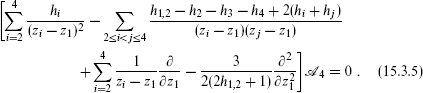
This differential equation is of hypergeometric form. The hypergeometric functions, however, are holomorphic (except for branch cuts at coincident points), while _1,2 has an unknown ₁ dependence. Now insert the expansion (15.2.9), in which the four-point correlation is written as a sum of terms, each a holomorphic conformal block times a conjugated block. The conformal blocks satisfy the same differential equation (15.3.5) and so are hypergeometric functions. Being second order, the differential equation (15.3.5) has two independent solutions, and each conformal block is a linear combination of these.

This procedure generalizes to any degenerate primary field. The primary _r,s will satisfy a generalization of the hypergeometric equation. This differential equation is of maximum order rs, coming from the term in the null state _r,s. If the antiholomorphic weight is also degenerate, = the antiholomorphic conformal blocks satisfy a differential equation of order , so that

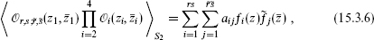
where f_i(z) and _j() are the general solutions of the holomorphic and antiholomorphic equations. The constants a_ij are not determined by the differential equation. They are constrained by locality — the holomorphic and antiholomorphic functions each have branch cuts, but the product must be single-valued — and by associativity. We will describe below some theories in which it has been possible to solve these conditions.

Let us see how the differential equation constrains the operator products of _1,2. According to the theory of ordinary differential equations, the points z₁ = z_i are regular singular points, so that the solutions are of the form (z₁ – z_i)^κ times a holomorphic function. Inserting this form into the differential equation and examining the most singular term yields the characteristic equation

This gives two solutions (z₁ – z_i)^κ± for the leading behavior as z₁ → z_i; comparing this to the OPE gives

for the primary fields in the _1,2i product. Parameterizing the weight by

the two solutions to the characteristic equation correspond to

These are the only weights that can appear in the operator product, so we have derived the fusion rule,

we have labeled the primary fields other than _1,2 by the corresponding parameter γ. A fusion rule is an OPE without the coefficients, a list of the conformal families that are allowed to appear in a given operator product (though it is possible that some will in fact have vanishing coefficient). For the operator _2,1, one obtains in the same way the fusion rule

In particular, for the product of two degenerate primaries this becomes

For positive values of the indices, the families on the right-hand side are degenerate. In fact, only these actually appear. Consider the fusion rule for _1,22,1. By applying the rule (15.3.13a) we conclude that only [_2,2] and [_2,0] may appear in the product, while the rule (15.3.13b) allows only [_2,2] and [_0,2]. Together, these imply that only [_2,2] can actually appear in the product. This generalizes: only primaries r ≥ 1 and s ≥ 1 are generated. The algebra of degenerate conformal families thus closes, and iterated products of _1,2 and _2,1 generate all degenerate _r,s. This suggests that we focus on CFTs in which all conformal families are degenerate.

The values of r and s are still unbounded above, so that the operator algebra will generate an infinite set of conformal families. When α_–/α₊ = –p/q is rational, the algebra closes on a finite set.² In particular, one then has

The point is that there is a reflection symmetry,

so that each conformal family has at least two null vectors, at levels rs and (p – r)(q – s), and its correlators satisfy two differential equations. The reflection of the conditions r > 0 and s > 0 is r < p and s < q, so the operators are restricted to the range

These theories, with a finite algebra of degenerate conformal families, are known as minimal models. They have been solved: the general solution of the locality, duality, and modular invariance conditions is known, and the operator product coefficients can be extracted though the details are too lengthy to present here.

Although the minimal models seem rather special, they have received a great deal of attention, as examples of nontrivial CFTs, as prototypes for more general solutions of the conformal bootstrap, as building blocks for four-dimensional string theories, and because they describe the critical behavior of many two-dimensional systems. We will return to several of these points later.

Let us now consider the question of unitarity. A necessary condition for unitarity is that all weights are nonnegative. One can show that this is true of the weights (15.3.14) only for q = p + 1. These are precisely the c < 1 representations (15.1.15) already singled out by unitarity:

Notice that these theories have been found and solved purely from symmetry, without ever giving a Lagrangian description. This is how they were discovered, though various Lagrangian descriptions are now known; we will mention several later. For m = 3, c is and there is an obvious Lagrangian representation, the free fermion. The allowed primaries,

are already familiar, being respectively the unit operator, the fermion ψ, and the R sector ground state.

The full minimal model fusion rules can be derived using repeated applications of the _2,1 and _1,2 rules and associativity. They are

For _p–1,1 only a single term appears in the fusion with any other field, _{p–1,1 r,s} = [_p–r,s]. A primary with these properties is known as a simple current. Simple currents have the useful property that they have definite monodromy with respect to any other primary. Consider the operator product of a simple current J(z) of weight h with any primary,

where J · [_i] = [_i′]. The terms with descendants bring in only integer powers of z, so all terms on the right pick up a common phase

when z encircles the origin. The charge Q_i, defined mod 1, is a discrete symmetry of the OPE. Using the associativity of the OPE, the operator product coefficient c^k_ij can be nonzero only if Q_i + Q_j = Q_k. Also, by taking repeated operator products of J with itself one must eventually reach the unit operator; suppose this occurs first for J^N. Then associativity implies that NQ_i must be an integer, so this is a Z_N symmetry. For the minimal models,

which is the identity, and so the discrete symmetry is Z₂. Evaluating the weights (15.3.21) gives

For the unitary case (15.3.17), exp(2πiQ_r,s) is (–1)^s–1 for m odd and (–1)^r–1 for m even.

Feigin–Fuchs representation

To close this section, we describe a clever use of CFT to generate integral representations of the solutions to the differential equations satisfied by the degenerate fields. Define

and consider the linear dilaton theory with the same value of the central charge,

The linear dilaton theory is not the same as a minimal model. In particular, the modes α_–k generate a Fock space of independent states, so the partition function is of order exp(π/6) as → 0, larger than that of a minimal model. However, the correlators of the minimal model can be obtained from those of the linear dilaton theory. The vertex operator

has weight α² – 2αα₀, so for

it is a primary of weight

For γ = rα₊ + sα_– it is then degenerate, and its correlator satisfies the same differential equation as the corresponding minimal model primary. There is a complication: the correlator

generally vanishes due to the conservation law

(derived in exercise 6.2). There is a trick which enables us to find a nonvanishing correlator that satisfies the same differential equation. The operators

are of weight (1, 0), so the line integral

known as a screening charge, is conformally invariant. Inserting into the expectation value, the charge conservation condition is satisfied for

Further, since the screening charges are conformally invariant, they do not introduce singularities into T(z) and the derivation of the differential equation still holds. Thus, the minimal model conformal blocks are represented as contour integrals of the correlators of free-field exponentials, which are of course known. This is the Feigin–Fuchs representation. It is possible to replace V_α → V_2α0–α in some of the vertex operators, since this has the same weight; one still obtains integer values of n_±, but this may reduce the number of screening charges needed. It may seem curious that the charges of the (1, 0) vertex operators are just such as to allow for integer n_±. In fact, one can work backwards, deriving the Kac determinant from the linear dilaton theory with screening charges.

The contours in the screening operators have not been specified — they may be any nontrivial closed contours (but must end on the same Riemann sheet where they began, because there are branch cuts in the integrand), or they may begin and end on vertex operators if the integrand vanishes sufficiently rapidly at those points. By various choices of contour one generates all solutions to the differential equations, as in the theory of hypergeometric functions. As noted before, one must impose associativity and locality to determine the actual correlation functions. The Feigin–Fuchs representation has been a useful tool in solving these conditions.

15.4 Current algebras

We now consider a Virasoro algebra L_k combined with a current algebra . We saw in section 11.5 that the Virasoro generators are actually constructed from the currents. We will extend that discussion to make fuller use of the world-sheet symmetry.

Recall that a primary state |r, i in representation r of g satisfies

As in the case of the Virasoro algebra, we are interested in highest weight representations, obtained by acting on a primary state with the L_m and for m < 0. As we have discussed, a CFT with a current algebra can always be factored into a Sugawara part and a part that commutes with the current algebra. We focus on the Sugawara part, where

Recall also that the central charge is

and that the weight of a primary state is

As in the Virasoro case, all correlations can be reduced to those of the primary fields. In parallel to the derivation of eq. (15.2.3), one finds

where

and so on for multiple raising operators. Here, t^a(i) acts in the representation r_i on the primary _i; the representation indices on t^a(i) and _i are suppressed.

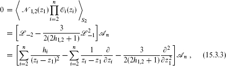
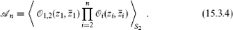
The Sugawara theory is solved in the same way as the minimal models. In particular, all representations are degenerate, and in fact contain null descendants of two distinct types. The first follows directly from the Sugawara form of T, which in modes reads

For m = –1, this implies that any correlator of primaries is annihilated by

This is the Knizhnik–Zamolodchikov (KZ) equation,

We have suppressed group indices on the primary fields, but by writing the correlator in terms of g-invariants, the KZ equation becomes a set of coupled first order differential equations — coupled because there is in general more than one g-invariant for given representations r_i. Exercise 15.5 develops one example. For the leading singularity (z₁ – z_i)^κ as z₁ → z_i, the KZ equation reproduces the known result (15.4.4) but does not give fusion rules. There is again a free-field representation of the current algebra (exercise 15.6), analogous to the Feigin–Fuchs representation of the Virasoro algebra.

The second type of null descendant involves the currents only, and does constrain the fusion rules. For convenience, let us focus on the case g = SU(2). The results can then be extended to general g by examining the SU(2) subalgebras associated with the various roots α. We saw in chapter 11 that the SU(2) current algebra has at least two interesting SU(2) Lie subalgebras, namely the global symmetry and the pseudospin

Now consider some primary field

which we have labeled by its quantum numbers under the global SU(2). What are its pseudospin quantum numbers (j′,m′)? Since it is primary, it is annihilated by the pseudospin lowering operator, so m′ = –j′. We also have m′ = m – k/2, so j′ = k/2 – m. Now, the pseudospin representation has dimension 2j′ + 1, so if we raise any state 2j′ + 1 times we get zero:

This is the null descendant.

Now take the correlation of this descendant with some current algebra primaries and use the relation (15.4.5) between the correlators of descendants and primaries to obtain

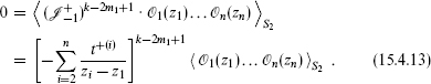
Notice that, unlike the earlier null equations, this one involves no derivatives and is purely algebraic. To see how this constrains the operator products, consider the three-point correlation. By considering the separate z_i dependences in eq. (15.4.13) one obtains

where we have now written out the group indices explicitly. This holds for all n₂ and n₃, and for

The matrix elements of (t⁺)^l are nonvanishing for at least some n_2,3 if m₂ ≥ l₂–j₂ and m₃ ≥ l₃ – j₃. Noting the restriction on l_2,3, we can conclude that the correlation vanishes when m₂ + m₃ ≥ k – 2m₁ + 1 – j₂ – j₃. Using m₁ + m₂ + m₃ = 0 and taking m₁ = j₁ (the most stringent case) gives

Although this was derived for m₁ = j₁, rotational invariance now guarantees that it applies for all m₁. Applying also the standard result for multiplication of SU(2) representations, we have the fusion rule

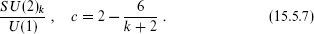
Again there is a simple current, the maximum value j = k/2:

The corresponding Z₂ symmetry is simply (–1)^2j.

Modular invariance

The spectrum of a g × g current algebra will contain some number n_r of each highest weight representation |r, . The partition function is then

with the character defined by analogy to that for the conformal algebra, eq. (15.2.12). Invariance under τ → τ + 1 amounts as usual to level matching, so n_r can be nonvanishing only when h_r – h is an integer. Under τ → –1/τ the characters mix,

so the condition for modular invariance is the matrix equation

The characters are obtained by considering all states generated by the raising operators, with appropriate allowance for degeneracy. Only the currents need be considered, since by the Sugawara relation the Virasoro generators do not generate any additional states. The calculation is then parallel to the calculation of the characters of finite Lie algebras, and the result is similar to the Weyl character formula. The details are too lengthy to repeat here, and we will only mention one simple classic result: the modular S matrix for SU(2) at level k is

The general solution to the modular invariance conditions is known. One solution, at any level, is the diagonal modular invariant for which each representation with j = appears once:

These are known as the A invariants. When the level k is even, there is another solution obtained by twisting with respect to (–1)^2j. One keeps the previous states with j integer only, and adds in a twisted sector where = k/2 – j. For k a multiple of 4, j in the twisted sector runs over integers, while for k + 2 a multiple of 4, j in the twisted sector runs over half-integers:

These are known as the D invariants. For the special values k = 10, 16, 28 there are exceptional solutions, the E invariants. The A–D–E terminology refers to the simply-laced Lie algebras. The solutions are in one-to-one correspondence with these algebras, the Dynkin diagrams arising in the construction of the invariants.

Strings on group manifolds

Thus far the discussion has used only symmetry, without reference to a Lagrangian. There is an important Lagrangian example of a current algebra. Let us start with a simple case, a nonlinear sigma model with a three-dimensional target space,

Let G_mn be the metric of a 3-sphere of radius r and let the antisymmetric tensor field strength be

for some constant q; _mnp is a tensor normalized to _mnp^mnp = 6. The curvature is

To leading order in α′, the nonvanishing beta functions (3.7.14) for this nonlinear sigma model are

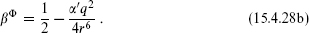
The first term in β^Φ is the contribution of three free scalars. The theory is therefore conformally invariant to leading order in α′ if

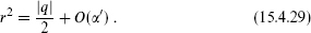
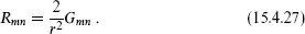
The central charge is

A 3-sphere has symmetry algebra O(4) = SU(2) × SU(2). In a CFT, we know that each current will be either holomorphic or antiholomorphic. Comparing with the SU(2) Sugawara central charge

the sigma model is evidently a Sugawara theory. One SU(2) will be left-moving on the world-sheet and one right-moving.

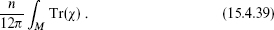
The general analysis of current algebras showed that the level k is quantized. In the nonlinear sigma model it arises from the Dirac quantization condition. The argument is parallel to that in section 13.3. A nonzero total flux H is incompatible with H = dB for a single-valued B. We can write the dependence of the string amplitude on this background as

where M is the embedding of the world-sheet in the target space and N is any three-dimensional manifold in S₃ whose boundary is M. In order that this be independent of the choice of N we need

Thus,

for integer n. More generally, ∫ H over any closed 3-manifold in spacetime must be a multiple of 4 π²α′.

This is the desired quantization, and |n| is just the level k of the current algebra. In particular, the one-loop central charge (15.4.30) becomes

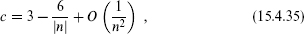
agreeing with the current algebra result to this order.

The 3-sphere is the same as the SU(2) group manifold, under the identification

The action (15.4.25) can be rewritten as the Wess–Zumino–Novikov–Witten (WZNW) action

where ω = g^–1dg is the Maurer–Cartan 1-form. Here M is the embedding of the world-sheet in the group manifold, and N is any 3-surface in the group manifold whose boundary is M. In this form, the action generalizes to any Lie group g. The second term is known as the Wess–Zumino term. The reader can check that

Therefore, locally on the group ω³ = dχ for some 2-form χ, and the Chern–Simons term can be written as a two-dimensional action

As with the magnetic monopole, there is no such χ that is nonsingular on the whole space.

The variation of the WZNW action is³

As guaranteed by conformal invariance, the global g × g symmetry

is elevated to a current algebra,

Left-multiplication is associated with a left-moving current algebra and right-multiplication with a right-moving current algebra. The currents are

Let us check that the Poisson bracket of two currents has the correct c-number piece. To get this, it is sufficient to expand

and keep the leading terms in the Lagrangian density and currents,

The higher-order terms do not contribute to the c-number in the Poisson bracket. The kinetic term now has the canonical α′ = 2 normalization so the level k = |n| follows from the normalization of the currents.

Which states appear in the spectrum? We can make an educated guess by thinking about large k, where the group manifold becomes more and more flat. The currents then approximate free boson modes so the primary states, annihilated by the raising operators, have no internal excitations — the vertex operators are just functions of g. The representation matrices form a complete set of such functions, so we identify

This transforms as the representation (r, r) under g×g, so summing over all r gives the diagonal modular invariant. Recall that for each k the number of primaries is finite; (g) for higher r evidently is not primary. This reasoning is correct for simply connected groups, but otherwise we must exclude some representations and add in winding sectors. For example, SU(2)/Z(2) = O(3) leads to the D invariant. We can understand the restriction to even levels for the D invariant: ∫ H on SU(2)/Z(2) is half of ∫ H on SU(2), so the coefficient must be even to give a well-defined path integral.

The group manifold example vividly shows how familiar notions of spacetime are altered in string theory. If we consider eight flat dimensions with both right- and left-moving momenta compactified on the E₈ root lattice, we obtain an E_8L × E_8R current algebra at level one. We get the same theory with 248 dimensions forming the E₈ group manifold with unit H charge.

15.5 Coset models

A clever construction allows us to obtain from current algebras the minimal models and many new CFTs. Consider a current algebra G, which might be a sum of several factors (g_i, k_i). Let H be some subalgebra. Then as in the discussion of Sugawara theories we can separate the energymomentum tensor into two pieces,

The central charge of T^G/H is

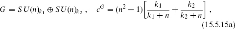
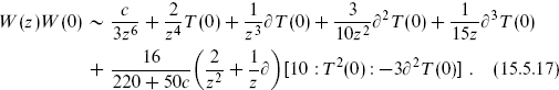
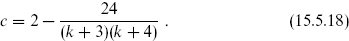
For any subalgebra the Sugawara theory thus separates into the Sugawara theory of the subalgebra, and a new coset CFT. A notable example is

where the subscripts denote the levels. Here, the H currents are the sums of the currents of the two SU(2) current algebras in G, j^a = + Then the central charges

are precisely those of the unitary minimal models with m = k + 2.

A representation of the G current algebra can be decomposed under the subalgebras,

where r is any representation of G, and r′ and r″ respectively run over all H and G/H representations, with nonnegative integers. For the minimal model coset (15.5.3), all unitary representations can be obtained in this way. The current algebra theories are rather well understood, so this is often a useful way to represent the coset theory. For example, while the Kac determinant gives necessary conditions for a minimal model representation to be unitary, the coset construction is regarded as having provided the existence proof, the unitary current algebra representations having been constructed directly. The minimal model fusion rules (15.3.19) can be derived from the SU(2) current algebra rules (15.4.17), and the minimal model modular transformation

can be obtained from the SU(2) result (15.4.22). Further, the minimal model modular invariants are closely related to the SU(2) A–D–E invariants.

Taking various G and H leads to a wealth of new theories. In this section and the next we will describe only some of the most important examples, and then in section 15.7 we discuss some generalizations. The coset construction can be regarded as gauging the subalgebra H. Conformal invariance forbids a kinetic term for the gauge field, and the equation of motion for this field then requires the H-charge to vanish, leaving the coset theory. This is the gauging of a continuous symmetry; equivalently, one is treating the H currents as constraints. Recall that gauging a discrete symmetry gave the orbifold (twisting) construction.

The parafermionic theories are:

Focusing on the U(1) current algebra generated by j³, by the OPE we can write this in terms of a left-moving boson H with standard normalization H(z)_H(0) ~x −ln z:

Operators can be separated into a free boson part and a parafermionic part. For the SU(2) currents themselves we have

where ψ₁ is known as the parafermionic current. Subtracting the weight of the exponential, the current has weight (k − 1)/k. One obtains further currents

with ψ_l having weight l(k −l)/k. The current algebra null vector (15.4.12) implies that ψ_l vanishes for l > k, which could also have been anticipated from its negative weight. The weight also implies that ψ₀ = ψ_k = 1, and from this one can also deduce that ψ_l = The current algebra primaries similarly separate,

where is a primary field of the parafermion algebra, and has weight j(j + 1)/(k + 2) − m²/k.

Factoring out the OPE of the free boson, the operator products of the parafermionic currents become

This algebra is more complicated than those encountered previously, in that the currents have branch cuts with respect to each other. However, it is simple in one respect: each pair of currents has definite monodromy, meaning that all terms in the operator product change by the same phase, exp(−4πill′/k), when one current circles the other. We will mention an application of the parafermion theories later.

For small k, the parafermion theories reduce to known examples. For k = 1, the parafermion central charge is zero and the parafermion theory trivial. In other words, at k = 1 the free boson is the whole SU(2) current algebra: this is just the torus at its self-dual radius. For k = 2, the parafermion central charge is , so the parafermion must be an ordinary free fermion. We recall from section 11.5 that SU(2) at k = 2 can be represented in terms of three free fermions. The free boson H is obtained by bosonizing ψ¹,², leaving ψ³ as the parafermion. At k = 3 the parafermion central charge is , identifying it as the m = 5 unitary minimal model.

Although constructed as SU(2) cosets, the minimal models have no SU(2) symmetry nor other any weight 1 primaries. In order for an operator from the G theory to be part of the coset theory, it must be nonsingular with respect to the H currents, and no linear combination of the currents and is nonsingular with respect to The situation becomes more interesting if we consider the bilinear invariants

In parallel with the calculations in exercise 11.7, the operator product of the H current with these bilinears is

The k = 0 term vanishes because the bilinear is G-invariant. For k = 1, commuting the lowering operator to the right gives a linear combination of and . All higher poles vanish. Thus, there are three bilinear invariants and only two possible singularities, so one linear combination commutes with the H current and lies entirely within the coset theory. This is just the coset energy-momentum tensor T^G/H, which we already know.

For SU(2) cosets that is the end of the story, but let us consider the generalization

For n ≥ 3 there is a symmetric cubic invariant

which vanishes for n = 2. Similarly, for n ≥ 4 there is an independent symmetric quartic invariant, and so forth. Using the cubic invariant, we can construct the four invariants The operator product with the H current has three possible singularities, so there must be one linear combination W(z) that lies in the coset theory. That is, the coset theory has a conserved spin-3 current. The states of the coset theory fall in representations of an extended chiral algebra, consisting of the Laurent modes of T(z), W(z), and any additional generators needed to close the algebra.

In general, the algebra contains higher spin currents as well. For example, the operator product W(z)W(0) contains a spin-4 term involving the product of four currents. For the special case n = 3 and k₂ = 1, making use of the current algebra null vectors, the algebra of T(z) and W(z) actually closes without any new fields. It is the W₃ algebra, which in OPE form is

In contrast to the various algebras we have encountered before, this one is nonlinear: the spin-4 term involves the square of T(z). This is the only closed algebra containing only a spin-2 and spin-3 current and was first discovered by imposing closure directly. It has a representation theory parallel to that of the Virasoro algebra, and in particular has a series of unitary degenerate representations of central charge

The (k₁, k₂, n) = (k, 1, 3) cosets produce these representations. As it happens, the first nontrivial case is k = 1, c = , which as we have seen also has a parafermionic algebra. The number of extended chiral algebras is enormous, and they have not been fully classified.

15.6 Representations of the N = 1 superconformal algebra

All the ideas of this chapter generalize to the superconformal algebras. In this section we will describe only the basics: the Kac formula, the discrete series, and the coset construction.

A highest weight state, of either the R or NS algebra, is annihilated by L_n and G_n for n > 0. The representation is generated by L_n for n < 0 and G_n for n ≤ 0. Each G_n acts at most once, since The Kac formula for the R and NS algebras can be written in a uniform way,

Here, is 1 in the R sector and 0 in the NS sector. The zeros are at

where r − s must be even in the R sector and odd in the NS sector. We have defined = 2c/3 and

The multiplicity of each zero is again the number of ways a given level can be reached by the raising operators of the theory,

Unitary representations are allowed at

and at the discrete series

where 1 ≤ r ≤ m − 1 and 1 ≤ s ≤ m + 1.

A coset representation for the N = 1 unitary discrete series is

The central charge is correct for m = k + 2. The reader can verify that the coset theory has N = 1 world-sheet supersymmetry: using the free fermion representation of the k = 2 factor, one linear combination of the (, 0) fields ψ^a and i^abcψ^aψ^bψ^c is nonsingular with respect to the H current and is the supercurrent of the coset theory.

For small m, some of these theories are familiar. At m = 2, c vanishes and we have the trivial theory. At m = 3, c = , which is the m = 4 member of the Virasoro unitary series. At m = 4, c = 1; this is the free boson representation discussed in section 10.7.

15.7 Rational CFT

We have seen that holomorphicity on the world-sheet is a powerful property. It would be useful if a general local operator of weight (h, ) could be divided in some way into a holomorphic (h, 0) field times an antiholomorphic (0, ) field, or a sum of such terms. The conformal block expression (15.2.9) shows the sense in which this is possible: by organizing intermediate states into conformal families, the correlation function is written as a sum of terms, each holomorphic times antiholomorphic. While this was carried out for the four-point function on the sphere, it is clear that the derivation can be extended to n-point functions on arbitrary Riemann surfaces. For example, the conformal blocks of the zero-point function on the torus are just the characters,

where counts the number of times a given representation of the left and right algebras appears in the spectrum.

When the sum is infinite this factorization does not seem particularly helpful, but when the sum is finite it is. In fact, in all the examples discussed in this section, and in virtually all known exact CFTs, the sum is finite. What is happening is that the spectrum, though it must contain an infinite number of Virasoro representations for c ≥ 1, consists of a finite number of representations of some larger extended chiral algebra. This is the definition of a rational conformal field theory (RCFT).

It has been conjectured that all rational theories can be represented as cosets, and that any CFT can be arbitrarily well approximated by a rational theory (see exercise 15.9 for an example). If so, then we are close to constructing the general CFT, but the second conjecture in particular seems very optimistic.

We will describe here a few of the general ideas and results. The basic objects in RCFT are the conformal blocks and the fusion rules, nonnegative integers which count the number of ways the representations i and j can be combined to give the representation k. For the Virasoro algebra, we know that two representations can be combined to give a third in a unique way: the expectation value of the primaries determines those of all descendants. For other algebras, may be greater than 1. For example, even for ordinary Lie algebras there are two ways to combine two adjoint 8s of SU(3) to make another adjoint, namely d^abc and f^abc. As a result, the same holds for the corresponding current algebra representations:

Repeating the derivation of the conformal blocks, for a general algebra the number of independent blocks is

where the repeated index is summed. Indices are lowered with = N_ij, zero denoting the identity representation. One can show that for each i, N_ij is nonvanishing only for a single j. This defines the conjugate representation, = 1. In the minimal models and SU(2) current algebra, all representations are self-conjugate, but for SU(n), n > 2 for example, they are not. By associativity, the s-channel conformal blocks are linearly related to the t-channel blocks The number of independent functions must be the same in each channel, so the fusion rules themselves satisfy an associativity relation,

We will now derive two of the simpler results in this subject, namely that the weights and the central charge must in fact be rational numbers in an RCFT. First note that the conformal blocks are not single-valued on the original Riemann surface — they have branch cuts — but they are single-valued on the covering space, where a new sheet is defined whenever one vertex operator circles another. Any series of moves that brings the vertex operators back to their original positions and sheets must leave the conformal blocks invariant. For example,

where τ_i…_j denotes a Dehn twist, cutting open the surface on a circle containing the indicated vertex operators, rotating by 2π and gluing. To see this, examine for example vertex operator 1. On the right-hand side, the combined effect of τ₁₂ and τ₁₃ is for this operator to circle operators 2 and 3 and to rotate by 4π. On the left, this is the same as the combined effect of τ4 (which on the sphere is the same as τ₁₂₃) and τ₁. eq. (15.7.4) is an N_ijkl-dimensional matrix equation on the conformal blocks. For example,

On the other hand, τ₁₃ is not diagonal in this basis, but rather in the dual basis

In order to get a basis-independent statement, take the determinant of eq. (15.7.4) and use (15.7.5) to get

This step is possible only when the number of primaries is finite.

There are many more equations than weights. Focusing on the special case i = j = k = l gives

This is − 1 equations for − 1 weights, where is the number of primaries; the weight h₀ is always 0, and the i = 0 equation is trivial. Let us consider the example of SU(2) current algebra at level 3, where there are four primaries, j = 0, , 1, . From the general result (15.4.17), the nonzero fusion rules of the form are

Thus we find that

are all integers, which implies that the weights are all rational. These results are consistent with the known weights j(j +1)/(k + 2). The reader can show that eqs. (15.7.7) are always nondegenerate and therefore require the weights to be rational.⁴

For the central charge, consider the zero-point function on the torus. The covering space here is just Teichmüller space, on which one may check that

The determinant of this implies that

The transformation T acts on the characters as

Thus,

and the rationality of c follows from that of the weights.

The consistency conditions for RCFT have been developed in a systematic way. Let us just mention some of the most central results. The first is the Verlinde formula, which determines the fusion rules in terms of the modular transformation S:

Indices are lowered with . The second is naturalness: any operator product coefficient that is allowed by the full chiral algebra is actually nonzero.⁵ The third result describes all possible modular invariants (15.7.1): either (the diagonal invariant), or where is some permutation symmetry of the fusion rules. The latter two results are not quite as useful as they sound, because they only hold with respect to the full chiral algebra of the theory. As we have seen in the W algebra coset example, this may be larger than one realizes.

Finally, let us mention a rather different generalization of the coset idea. Suppose we have a current algebra G, and we consider all (2, 0) operators formed from bilinears in the currents,

The condition that the TT OPE has the correct form for an energymomentum tensor, and therefore that the modes of T form a Virasoro algebra, is readily found. It is the Virasoro master equation,

where k^ab is the coefficient 1/z² in the current–current OPE. The central charge is

We already know some solutions to this: the Sugawara tensor for G, or for any subalgebra H of G. Remarkably, the set of solutions is very much larger: for G = SU(3)k, the number has been estimated as billion for each k. For each solution the G theory separates into two decoupled theories, with energy-momentum tensors T′ and T^G − T′. Some of these may be equivalent to known theories, but others are new and many have irrational central charge.

15.8 Renormalization group flows

Consistent string propagation requires a conformally invariant world-sheet theory, but there are several reasons to consider the relation of CFTs to the larger set of all two-dimensional field theories. First, CFT also has application to the description of critical phenomena, where the parameters can be varied away from their critical values. Second, there is a rich mathematical and physical interplay between conformal theories and nearby nonconformal ones, each illuminating the other. Third, conformally invariant theories correspond to string backgrounds that satisfy the classical equations of motion. One might then guess that the proper setting for quantum string theory would be a path integral over all background field configurations — that is, over all two-dimensional quantum field theories. This last is more speculative; it is related to other formulations of string field theory, a subject discussed briefly in chapter 9.

In this section we will develop some general results relating conformal and nonconformal theories. In the next we will discuss some examples and applications. Once again, this is an enormous subject and we can only sketch a few of the central ideas and results.

Scale invariance and the renormalization group

Consider the scale transformation

on a world-sheet with flat metric g_ab = δab. Alternatively we could keep the coordinates fixed and scale up the metric,

In either form the net change (3.4.6) in the action and measure is

A flat world-sheet theory will therefore be scale-invariant provided that

for some local operator .

Scale invariance plays an important role in many parts of physics. One expects that the extreme low energy limit of any quantum field theory will approach a scale-invariant theory. This has not been proven in general, but seems to be true in all examples. The scale-invariant theory may be trivial: if all states are massive then at low enough energy nothing is left. Consider for example a statistical mechanical system. The Boltzmann sum is the same as the Euclidean path integral in quantum field theory. This may have an energy gap for generic values of the parameters and so be trivial at long distance, but when the parameters are tuned to send the gap to zero (a second order phase transition) it is described by a nontrivial scale-invariant theory.

The term nontrivial in this context is used in two different ways. The broad usage (which is applied in the previous paragraph) means any field theory without an energy gap, so that there are states of arbitrarily small nonzero energy. A narrower usage reserves the term for scaleinvariant theories with interactions that remain important at all distances, as opposed to those whose low energy limit is equivalent to that of a free field theory.

Scale and conformal invariances are closely related. The scale transformation rescales world-sheet distances by a constant factor, leaving angles and ratios of lengths invariant. A conformal transformation rescales worldsheet distances by a position-dependent factor; on a very small patch of the world-sheet it looks like a scale transformation. In particular, conformal transformations leave angles of intersection between curves invariant. Comparing the condition (15.8.4) with the condition T^a_a = 0 for conformal invariance, one sees that it is possible in principle for a theory to be scale-invariant without being conformally-invariant. However, it is difficult to find examples. Later in the section we will prove that for compact unitary CFTs in two dimensions scale invariance does imply conformal invariance. Exercise 15.12 gives a nonunitary counterexample.

This is of some importance in dimensions greater than two. In the previous chapter we encountered two nontrivial (in the narrow sense) scale-invariant theories. The first was the d = 4, N = 4 gauge theory. The second was the d = 6 (2, 0) tensionless string theory, which arose on coincident IIA or M-theory 5-branes. Both are believed to be conformally invariant.

In quantum field theory, the behavior of matrix elements under a rigid scale transformation is governed by a differential equation, the renormalization group equation. Let us derive such an equation. Consider a general quantum field theory in d-dimensional spacetime; spacetime here corresponds to the string world-sheet, which is the case d = 2. The scale transformation of a general expectation value is

where _i is a complete set of local operators. The second term is from the action of the scale transformation on the operators,

The integrated trace of the energy-momentum tensor can be expanded in terms of the complete set,

The prime on the sum indicates that it runs only over operators with dimension less than or equal to d, because this is the dimension of the energy-momentum tensor. We can similarly write a general renormalizable action as a sum over all such terms

Here gⁱ is a general notation that includes the interactions as well as the masses and the kinetic term normalizations. The expansions (15.8.7) and (15.8.8) can be used to rewrite the scale transformation (15.8.5) as the renormalization group equation,

There may also be contact terms between T^a_a and the other operators, and terms from the g_i-derivative acting on the local operators. These are dependent on definitions (the choice of renormalization scheme) and can all be absorbed into the definition of Δ_i^j. eq. (15.8.9) states that a scale transformation is equivalent to a change in the coupling plus a mixing of operators. As one looks at longer distances the couplings and operators flow.

The Zamolodchikov c-theorem.

Without conformal invariance, T_zz is not holomorphic, its modes do not generate a Virasoro algebra, and the central charge c is not defined. Nevertheless, c has a useful extension to the space of all two-dimensional field theories.

Define

Rotational invariance implies that these depend only on as indicated. From conservation, one finds that

where a dot denotes differentiation with respect to ln r². The Zamolodchikov C function is the combination

This has the property

In a unitary theory H can be written as a sum of absolute squares by inserting a complete set of states, and so is nonnegative. The result (15.8.13) shows that the physics changes in a monotonic way as we look at longer and longer distances. Also, C is stationary if and only if the two-point function of with itself is zero, implying (by a general result in unitary quantum field theory) that itself vanishes identically. The theory is then conformally invariant and C becomes precisely c.

The monotonicity property also implies that the theory at long distance will approach a stationary point of C and therefore a CFT Again, this is intuitively plausible: at long distances the theory should forget about underlying distance scales. In general this is likely to happen in the trivial sense that all fields are massive and only the empty c = 0 theory remains. However, if massless degrees of freedom are present due to some combination of symmetry and the tuning of parameters, the c-theorem implies that their interactions will be conformally invariant. We should emphasize that the unitarity and compactness are playing a role; in the more general case there do exist counterexamples (exercise 15.12).

Like c, the C function seems to represent some generalized measure of the density of states. The monotonicity is then very plausible: a massive field would contribute to the number of degrees of freedom measured at short distance, but drop out at distances long compared to its Compton wavelength. In spite of this intuitive interpretation, there seems to be no simple generalization of the C function to d > 2. However, the principle that the long distance limit of any quantum field theory is conformally invariant still seems to hold under broad conditions.

Conformal perturbation theory

Now let us consider adding small conformally-noninvariant terms to the action of a CFT,

where S₀ is the action of the CFT. For convenience we focus on the case that the perturbations are primary fields, but the results are easily generalized. The λⁱ are the earlier couplings gⁱ minus the value at the conformal point.

The main question is how the physics in the perturbed theory depends on scale. Consider the following operator product, which arises in first order perturbation theory for correlations of the energy-momentum tensor:

We have

Integrating this, the first order perturbation (15.8.15) implies that perturbation leads to

As expected, the energy-momentum tensor is no longer holomorphic, unless the perturbation is of weight h_i = 1. The energy-momentum tensor must still be conserved,

Inspection of the divergence (15.8.17) thus identifies

We assume that the perturbations are rotationally invariant, so that T_ab remains symmetric.

Referring back to the renormalization group, we have

so that a rescaling of lengths by is equivalent to a rescaling of the couplings,

A perturbation with h_i > 1 is thus termed irrelevant, because its effect drops away at long distance and we return to the conformal theory. A perturbation with h_i < 1 is termed relevant. It grows more important at low energies, and we move further from the original conformal theory. A perturbation with h_i = 1 is termed marginal.

Now let us go to the next order in g. Consider first the case that the perturbations _i are all of weight (1, 1), marginal operators. Second order perturbation theory will then involve the operator product

the factor of coming from the expansion of exp(−S). The part of the OPE that involves only marginal operators is

so the second order term (15.8.22) will have a logarithmic divergence when z → w,

The divergence must be cut off at the lower end, introducing a scale into the problem and breaking conformal invariance. At the upper end, the scale is set by the distance at which we are probing the system. We can read off immediately the scale dependence: if we increase the scale of measurement by a factor 1 + , the log increases by . This is equivalent to shifting the couplings by

In other words,

As an application, suppose that we are interested in perturbations that preserve conformal invariance. We have the familiar necessary condition that the perturbation be a (1,1) tensor, but now we see that there are further conditions: conformal invariance will be violated to second order in λ unless

for all (1,1) operators k.

Now we wish to go to second order in λ for perturbations that are not marginal. At weak coupling, the order λ² term is important only if the first order term is small — that is, if the coupling is nearly marginal. To leading order in h_i − 1, we can just carry over our result for O(λ²) in the marginal case. Combining the contributions (15.8.20) and (15.8.26), we then have

with corrections being higher order in h_i − 1 or λⁱ. Let us also work out the C function. With the result (15.8.13) for the C function becomes to leading order

where

is evaluated at λⁱ = 0. Observe that

indices being lowered with G_ij. Using this and βⁱ = −2λⁱ gives

This integrates to

with c being the central charge at the conformal point λⁱ = 0.

Now let us apply this to the case of a single slightly relevant operator,

normalized so that G₁₁ = 1. If λ starts out positive it grows, but not indefinitely: the negative second order term cuts off the growth. At long distance we arrive at a new conformal theory, with coupling

From the string spacetime point of view, we can interpret U(λ) as a potential energy for the light field corresponding to the world-sheet coupling λ, and the two conformal theories correspond to the two stationary points of the cubic potential. Note that λ = 0 is a local maximum: relevant operators on the world-sheet correspond to tachyons in spacetime. The central charge of the new fixed point is

15.9 Statistical mechanics

The partition function in classical statistical mechanics is

where the integral runs over configuration space, β is the inverse temperature, and the Hamiltonian H is the integral of a local density. This has a strong formal similarity to the path integral for Euclidean quantum theory,

In the statistical mechanical case, the configuration is a function of the spatial dimensions only, so that statistical mechanics in d spatial dimensions resembles quantum field theory in d spacetime dimensions. An obvious difference between the two situations is that in the statistical mechanical case there is generally an underlying discrete structure, while in relativistic field theory and on the string world-sheet we are generally interested in a continuous manifold.

There is a context in statistical mechanics in which one essentially takes the continuum limit. This is in critical phenomena, in which some degrees of freedom have correlation lengths very long compared to the atomic scale, and the discrete structure is no longer seen. In this case, the statistical ensemble is essentially identical to a relativistic field theory. Let us discuss the classic example, the Ising model. Here one has an array of spins on a square lattice in two dimensions, each spin σ_i taking the values ±1. The energy is

The sum runs over all nearest-neighbor pairs (links). The energy favors adjacent pairs being aligned. When β is small, so that the temperature is large, the correlations between spins are weak and short-range,

as the distance |i − j| goes to infinity. For sufficiently large β the Z₂ symmetry σ_i → −σ_i is broken and there is long-range order,

For both small and large β the fluctuations are short-range. However, the transition between these behaviors is second order, both ξ(β) and ξ′(β) going to infinity at the critical value β_c. At the critical point the falloff is power law rather than exponential,

The long-wavelength fluctuations at this point should be described by a continuum path integral. The value of the critical exponent η is known from the exact solution of the Ising model to be . This cannot be deduced from any classical reasoning, but depends in an essential way on the nonlinear interactions between the fluctuations.

To deduce the CFT describing the critical theory, note the global symmetry of the Ising model, the Z₂ symmetry σ_i → −σ_i. We have a whole family of CFTs with this symmetry, the minimal models. For reasons to be explained below, the correct minimal model is the first nontrivial one, m = 3 with c = . The nontrivial primary fields of this theory, taking into account the identification (15.3.15), are

Under the Z₂ (15.3.23), _1,2 is odd and the other two are even. In particular, the Ising spins, being odd under Z₂, should evidently be identified as

The left- and right-moving factors must be the same to give a rotationally invariant operator. There are separate Z₂s acting on the left- and right-moving theories, but all operators have equal left and right charges so we can take either one. The expectation value

agrees with the exact solution for the critical exponent η.

The m = 3 minimal model is equivalent to the free massless Majorana fermion. Indeed, Onsager solved the Ising model by showing that it could be rewritten in terms of a free fermion on a lattice, which in general is massive but which becomes massless at β_c. Note that _1,3 has the correct dimension to be identified with the fermion field, and _1,2 has the correct dimension to be the R sector ground state vertex operator for a single Majorana fermion.

Incidentally, the solubility of the Ising model for general β can be understood directly from the CFT. Changing the temperature is equivalent to adding

to the action. This is the only relevant perturbation that is invariant under the Z₂ symmetry. This perturbation breaks the conformal invariance, but it can be shown from the OPEs of the CFT that a spin-4 current constructed from is still conserved. The existence of a symmetry of spin greater than 2 in a massive theory is sufficient to allow a complete solution. Of course, in the present case the perturbation (15.9.10) is just a mass for the free fermion, but for other CFTs without such a simple Lagrangian description this more abstract approach is needed.

The requirement that operators have integer spin means that we can only pair the same conformal family on the right and left. For the theory quantized on the circle, this corresponds to the A modular invariant discussed earlier,

In terms of the free fermion theory this is the diagonal GSO projection.

For two-dimensional critical theories with few enough degrees of freedom that the central charge is less than one, the classification of unitary representations of the Virasoro algebra completely determines the possible critical exponents: they must be given by one of the minimal models.⁶ For this reason this same set of CFTs arises from many different short-distance theories. Let us mention one such context, which illustrates the relation among all the unitary minimal models through the Z₂ symmetry they share. We noted that the m = 3 theory has only one relevant perturbation that is invariant under Z₂. We therefore identified this with a variation of the temperature away from the critical point. The operator _1,11,1 is just the identity and adding it to the action has a trivial effect. The operator _1,21,2 is odd under Z₂ and corresponds to turning on a magnetic field that breaks the σ_i → −σ_i symmetry. For the minimal model at general m there are m − 2 nontrivial relevant Z₂-invariant operators. This corresponds to multicritical behavior. To reach such a model one must tune m − 2 parameters precisely.

For example, take the Ising model with thermally equilibrated (annealed) vacancies, so that each spin σ can take values ±1 or 0, the last corresponding to an empty site. When the density ρ of vacancies is small, the behavior is much like the Ising model, with the same critical behavior at some point β_c(ρ). However, when the vacancy density reaches a critical value ρ_c, then at β_c(ρ_c) there are independent long-range fluctuations of the spin and density. This is known as the tricritical Ising model, tricritical referring to the need to adjust two parameters to reach the critical point. Since there are more long-range degrees of freedom than in the Ising model, we might expect the critical theory to have a greater central charge. The tricritical Ising model has been identified with the next minimal model, m = 4 with This generalizes: with spins (also called ‘heights’) taking m − 1 values, there is a multicritical point obtained by adjusting m − 2 parameters which is described by the corresponding minimal model. In fact, every CFT we have described in this chapter can be obtained as the critical limit of a lattice theory, and indeed of a solvable lattice theory. It is quite likely that every rational theory can be obtained from a solvable lattice theory.

A different generalization of the Ising model is the Z_k Ising model (the clock model). Here the spins take k values σ_i = exp(2πin/k) for n = 0, 1, ..., k − 1, and there is a Z_k symmetry σ_i → exp(2πi/k)σ_i. The energy is

Again there is a critical point at a value β_c. The critical behavior is described by the Z_k parafermion theory. The Z_k parafermions describe a generic critical system in which the fluctuations transform under a Z_k symmetry.

Several of the low-lying minimal models can be realized in different ways. The m = 5 theory is obtained as a four-height Z₂ model or a Z₃ Ising model. It is also known as the three-state Potts model, referring to a different generalization of the Ising model (spins taking k values with a permutation symmetry S_k) which happens to be the same as the Z_k generalization when k = 3. The m = 6 model can be obtained as a five-height Z₂ model or as a tricritical point of the Z₃ Potts/Ising model with vacancies. In fact the m = 3, 4, 5, 6 theories have all been realized experimentally, usually in systems of atoms adsorbed on surfaces. Since the m = 4 model is also the m = 3 minimal model of the N = 1 supersymmetric series, this is in a sense the first experimental realization of supersymmetry. (Some atomic and nuclear systems have an approximate Fermi/Bose symmetry, but this is a nonrelativistic algebra whose closure does not involve the translations.)

Landau–Ginzburg models

To complete this section, we will give a slightly different Lagrangian description of the minimal models. To study the long-wavelength behavior of the Ising model, we can integrate out the individual spins and work with a field representing the average spin over a region of many sites. This field takes essentially continuous values, rather than the original discrete ones. The first few terms in the Lagrangian density for would be

At λ₁ = 0 the tree-level mass of the field is zero. We thus identify λ₁ as being proportional to β_c − β, with λ₁ = 0 being the critical theory, the m = 3 minimal model.

This is the Landau–Ginzburg description. The original idea was that the classical potential for represented the free energy of the system. Now one thinks of this as the effective Lagrangian density for a full quantum (or thermal) path integral. The quantum or thermal fluctuations cannot be neglected. In some systems, though not here, they change the transition from continuous to discontinuous, so that there is no critical behavior. In general they significantly modify the scaling properties (critical exponents).

Now add a λ₃⁶ term and tune λ₁ and λ₂ to zero. We might expect a different critical behavior — the potential is flatter than before, so will have more states below a given energy, but it is still positive so there will be fewer states than for a free scalar. In other words, we guess that c is more than and less than 1. It is natural to identify this with the next minimal model, the m = 4 tricritical Ising model, since the number of relevant Z₂-invariant perturbations is two. Similarly, we guess that the Landau–Ginzburg model whose leading potential is ^2m−2 represents the mth minimal model.

Representing the minimal models by a strongly interacting quantum field theory seems to have little quantitative value, but it gives an intuitive picture of the operator content. To start we guess that corresponds to the operator of lowest dimension, namely _2,2. Also, we guess that we have the diagonal theory, so the left-moving representation is the same as the right-moving one, and we indicate only the latter. Now, to find ², use the fusion rule

The first term is the identity; we guess that ² is the remaining operator of lowest dimension, namely _3,3. Taking further products with _2,2, we identify

This terminates due to the upper bound (15.3.16), r ≤ m − 1. The lowest term in · ^m−2 is _m,m−2 which by reflection is _1,2. We then continue

All this guesswork can be checked in various ways. One check is that the Z₂ symmetry assignment (15.3.23), namely (−1)^s for m odd and (−1)^r for m even, matches that of ⁿ. As another check, where is the next monomial ^2m−3? The product · ^2m−4 leads to no new primaries. This is just right: the equation of motion is

so this operator is a descendant. The powers (15.9.15) and (15.9.16) are all the relevant primary operators.

What happens if we add a relevant perturbation to the Lagrangian for the mth minimal model? The Landau–Ginzburg picture indicates that adding ^2k−2 causes the theory to flow to the kth minimal model. Let us consider in particular ^2m−4 for m large. This is

which is nearly marginal. Thus we can apply the formalism of the previous section. From the fusion rule

the only nearly marginal operator in _{1,3 1,3} is _1,3 itself, so we are in precisely the single-operator situation worked out in the last paragraph of the previous section. Thus, we can construct a new conformal theory by a small _1,3 perturbation of the minimal model. The Landau–Ginzburg picture indicates that this is the next minimal model down. We can compute the central charge from the c-theorem. Taking from the literature the value c₁₁₁ = 4/3^1/2 for the large-m minimal model yields

For large m this is indeed the difference between the central charges of successive minimal models.

Exercises

15.1 Evaluate det and compare with the Kac formula.

15.2 Derive eqs. (15.2.3) and (15.2.5) for the expectation value of a descendant.

15.3 Work out the steps outlined in the derivation of eq. (15.2.9) to find explicitly the N = 0 and N = 1 terms in

15.4 Verify that the discrete symmetries associated with the simple currents are as asserted below eqs. (15.3.23) and (15.4.18) for the unitary minimal models and the SU(2) WZNW models.

15.5 (a) For the SU(n) current algebra at level k, consider the four-point function with two insertions in the representation (n, n) and two in the representation Find the KZ equation for the SU(n) invariants.

(b) Find the general solution for k = 1 and determine the coefficients using associativity and locality. Compare this with the free-boson representation.

(c) Do the same for general k; the solution involves hypergeometric functions.

15.6 The Wakimoto representation is a free-field representation for the SU(2) current algebra, analogous to the Feigin–Fuchs representation of the minimal models. Show that the following currents form an SU(2) current algebra of level k = q²−2:

Here w,χ are a commuting β_γ system and is a free scalar. Show that the Sugawara energy momentum tensor corresponds to the β_γ theory with h_w = 1 and h_χ = 0, and with being a linear dilaton theory of appropriate central charge.

15.7 For the coset construction of the minimal models, combine primary fields from the two factors in G to form irreducible representations of SU(2). Subtract the weight of the corresponding primary of H and show that the resulting weight is one of the allowed weights for the minimal model. Not all minimal model primaries are obtained in this way; some are excited states in the current algebras.

15.8 Repeat the previous exercise for the coset construction of the minimal N = 1 superconformal theories.

15.9 For the periodic scalar at any radius, the analysis in section 15.2 shows that the spectrum contains an infinite number of conformal families. Show, however, that if R²/α′ is rational, the partition function is a sum of a finite number of factors, each one holomorphic times antiholomorphic in τ. Show that at these radii there is an enlarged chiral algebra.

15.10 Apply the result (15.7.7) to the SU(2) current algebra at k = 4. Show that the resulting relations are consistent with the actual weights of the SU(2) primaries.

15.11 Verify the Verlinde formula (15.7.14) for the SU(2) modular transformation (15.4.22). In this case indices are raised with the identity matrix.

15.12 For the general massless closed string vertex operator, we found the condition for Weyl invariance in section 3.6. Find the weaker condition for invariance under rigid Weyl transformations, and find solutions that have only this smaller invariance.

¹ By contrast, a unitary representation is always irreducible. The reader can show that the lowest state in any invariant subspace would have to be orthogonal to itself, and therefore vanish.

² Note that α₊α_– = –1, and that 0 > α_–/α₊ > –1.

³ This is for n > 0; for n < 0 interchange z and .

⁴ We are assuming that all the N_iiii are nonzero. More generally, one can derive a similar relation with which is always positive.

⁵ This precise statement holds only when the are restricted to the values 0 and 1; otherwise, it requires some refinement.

⁶ There is a caveat: the CFTs that arise in statistical physics need not be unitary. Unitarity in that context is related to a property known as reflection positivity, which holds in most but not all systems of interest.