13

D-branes

In chapter 8 we found that a number of new phenomena, unique to string theory, emerged when the theory was toroidally compactified. Most notable were the T-duality of the closed oriented theory and the appearance of D-branes in the R → 0 limit of the open string theory. These subjects become richer still with the introduction of supersymmetry. We will see that the D-branes are BPS states and carry R-R charges. We will argue that the type I, IIA, and IIB string theories are actually different states in a single theory, which also includes states containing general configurations of D-branes. Whereas previously we considered only parallel D-branes all of the same dimension, we now wish to study more general configurations. We will be concerned with the breaking of supersymmetry, the spectrum and effective action of strings stretched between different D-branes, and scattering and bound states of D-branes. In the present chapter we are still in the realm of string perturbation theory, but many of the results will be used in the next chapter to understand the strongly coupled theory.

13.1 T-duality of type II strings

Even in the closed oriented type II theories T-duality has an interesting new effect. Compactify a single coordinate X⁹ in either type II theory and take the R → 0 limit. This is equivalent to the R → ∞ limit in the dual coordinate, whose right-moving part is reflected

just as in the bosonic string. By superconformal invariance we must also reflect ,

However, this implies that the chirality of the right-moving R sector ground state is reversed: the raising and lowering operators are interchanged. Simply put, T-duality is a spacetime parity operation on just one side of the world-sheet, and so reverses the relative chiralities of the right- and left-moving ground states. If we begin with the IIA theory and take the compactification radius to be small, we obtain the IIB theory at large radius, and vice versa. The same is true if we T-dualize — that is, carry out the change of variables (13.1.1) and (13.1.2) — on any odd number of dimensions, while T-dualizing on an even number returns one to the type II theory with which one began. Thus the two type II theories are related in the same way as the two heterotic theories: in each case the two noncompact theories are different limits of a single space of compactified theories. The type II relation is even simpler than the heterotic relation, in that one takes the radius to zero without having also to include a Wilson line.

Since the IIA and IIB theories have different R–R fields, T-duality must transform one set into the other. Again focus on T-duality in just the 9-direction. In order to preserve the OPE between ^µ and the spin field, this must act as

where β⁹ is the parity transformation (9-reflection) on the spinors. It anticommutes with Γ⁹ and commutes with the remaining Γ^µ, so β⁹ = Γ⁹Γ. Now consider the effect on the R–R vertex operators

The T-duality multiplies the product of Γ matrices by Γ⁹Γ on the right. The Γ just gives ±1 because the R ground states have definite chirality. The Γ⁹ adds a ‘9’ to the set µ₁ ... µ_p if none is present, or removes one if it is present via (Γ⁹)² = 1. This is how T-duality acts on the R–R field strengths and potentials, adding or subtracting the index for the dualized dimensions. Thus, if we start from the IIA string we get the IIB R–R fields as follows (up to signs),

where here µ stands for a nondualized dimension. We could go on, getting C_µνλω from C_µνλω9 and so on, but these are not independent fields, and give rather the Poincaré dual description of the fields listed.

For T-duality on multiple dimensions replace β⁹ with

where β^m = ΓΓ^m and the product runs over the dualized directions. There are some signs which should be noted but should not distract attention from the main physical point. Since β^mβⁿ = —βⁿβ^m for m ≠ n, T-dualities in different directions do not quite commute but differ by a sign in the right-moving R sector. We can write this as

where is the spacetime fermion number of the right-moving state of the string; this is a symmetry that flips the sign of all right-moving R states. Also, we have defined β^m so as to preserve the Hermiticity of (that is, it is real in a Majorana basis), but then β^mβ^m = –1 and so acting twice with T-duality gives exp(πi).

13.2 T-duality of type I strings

Taking the R → 0 limit of the open and unoriented type I SO(32) theory leads to D-branes and orientifold planes by the same arguments as for the bosonic string in chapter 8, which the reader should review. In particular, taking the T-dual on a single dimension leads to a space with 16 D8-branes between two orientifold hyperplanes.

Let us first consider the bulk physics of the T-dual theory, obtained by taking R → 0 and concentrating on a region of the dual spacetime that is far away from the fixed planes and D-branes, as illustrated in figure 13.1. The local physics is that of a closed oriented superstring theory: closed because the open strings live far away on the D-branes; oriented because the orientation projection relates the state of any string to that of its image behind the fixed plane, but does not locally constrain the space of states. Thus the local physics must be that of a type II theory. In particular there are two gravitinos, and any closed string scattering process will be invariant under the 32 supersymmetries of the type II theory. Since the type I theory with which we started has equal left- and right-moving chiralities, taking the T-dual in one dimension makes them opposite: the local physics is the IIA superstring. Taking the T-dual on any odd number of dimensions has the same effect; taking the T-dual on any even number of dimensions gives the IIB theory in the bulk.

Now take the R → 0 limit while concentrating on the neighborhood of one D-brane in the T-dual theory, adjusting the Wilson lines so that again the fixed plane and other D-branes move away in the T-dual spacetime. The low energy degrees of freedom on the D-brane are the massless open string states

Fig. 13.1. A D-brane, with one attached open string and one closed string moving in the bulk. The physics away from the D-brane is described by a type II string theory, so the string theory with the D-brane has the physical properties of a state of the type II theory containing an extended object.

As in the bosonic theory, the bosonic states are a gauge field living on the D-brane and the collective coordinates for the D-brane. The fermionic states are the superpartners of these.

Consider now a process where closed strings scatter from the D-brane; this necessarily involves a world-sheet with boundary. Now, the open string boundary conditions are invariant only under d = 10, N = 1 supersymmetry. In the original type I theory, the left-moving world-sheet current for spacetime supersymmetry flows into the boundary and the right-moving current flows out, so only the total charge Q_α + _α of the left- and right-movers is conserved. Under T-duality this becomes

The scattering amplitudes of closed strings from the D-brane are invariant only under these 16 supersymmetries.

To see the significance of this, consider first the conservation of momentum. There is a nonzero amplitude for a closed string to reflect backwards from the D-brane, which clearly does not conserve momentum in the direction orthogonal to the D-brane. This occurs because the Dirichlet boundary conditions explicitly break translational invariance. However, from the spacetime point of view the breaking is spontaneous: we are expanding around a D-brane in some definite location, but there are degenerate states with the D-brane translated by any amount.¹ For a spontaneously broken symmetry the consequences are more subtle than for an unbroken symmetry: the apparent violation of the conservation law is related to the amplitude to emit a long-wavelength Goldstone boson. For the D-brane, as for any extended object, the Goldstone bosons are the collective coordinates for its motion. In fact, the nonconservation of momentum is measured by the integral of the corresponding current over the world-sheet boundary,

which up to normalization is just the (0 picture) vertex operator for the collective coordinate, with zero momentum in the Neumann directions.

We conclude by analogy that the D-brane also spontaneously breaks 16 of the 32 spacetime supersymmetries, the ones that are explicitly broken by the open string boundary conditions. The integrals

which measure the breaking of supersymmetry, are just the vertex operators for the fermionic open string state (13.2.1). Thus this state is a goldstino, the Goldstone state associated with spontaneously broken supersymmetry.

It is not surprising that the D-brane breaks some supersymmetry. The only state invariant under all supersymmetries is the vacuum. Rather, what is striking is that it leaves half the supersymmetries unbroken: it is a BPS state. This same argument holds for any number of dualized dimensions, and so for Dp-branes for all p. The unbroken supersymmetry is

where

the product running over all the dimensions perpendicular to the D-brane.

BPS states, which are discussed in section B.2, must carry conserved charges. In the present case there is a natural set of charges with the correct Lorentz properties, namely the antisymmetric R–R charges. The world-volume of a p-brane naturally couples to a (p + 1)-form potential

the integral running over the D-brane world-volume. By T-duality we can reach the IIA theory with a Dp-brane of any even p. Thus we need 1-, 3-, 5-, 7-, and 9-form potentials. Indeed, the 1-form and 3-form are in the IIA theory and the 5-form and 7-form give equivalent descriptions of the same physics. The 9-form potential we have discussed in section 12.1 in the context of massive IIA supergravity. Although it is not associated with propagating states, and so was not detected in the quantization of the IIA string, the existence of D8-branes shows that it must be included.

By analogy with electromagnetism in four dimensions, where the 1-form electric potential can be replaced with a 1-form magnetic potential, a Dirichlet p-brane and (6 – p)-brane are like electric and magnetic sources for the same field strength. For example, the free field equation and Bianchi identity for a 2-form field strength, d∗F₂ = dF₂ = 0, are symmetric between F₂ and (∗F)₈, and can be written either in terms of a 1-form or 7-form potential:

At an electric source, which would be a D0-brane for C₁ or a D6-brane for C₇, the field equation has a source term. At a magnetic source, a D6-brane for C₁ or a D0-brane for C₇, the Bianchi identity breaks down, and the potential cannot be globally defined: one must introduce a Dirac string, or use different potentials in different patches.²

For the IIB theory we need 2-, 4-, 6-, 8-, and 10-form potentials. The first four arise in either the electric or magnetic description of the propagating R–R states. The existence of the 10-form was deduced in section 10.8, from the study of type I divergences. Indeed, we argued there for the coupling (13.2.7) for the 10-form, where the integral runs over all spacetime. This fits with a point made in chapter 8, that it is natural to interpret each Chan–Paton degree of freedom in the fully Neumann theory as a 9-brane filling spacetime. All the other R–R couplings follow from this one by T-duality, since each time we T-dualize in an additional direction the dimension of the p-branes goes down by one and the R–R form loses an index.

The IIB theory also has a 0-form potential C₀, the R–R scalar. This should couple to a ‘(−1)-brane.’ Indeed, there is a natural interpretation to this: it is defined by Dirichlet boundary conditions in all directions, time as well as space, so its world-sheet is zero-dimensional and the integral (13.2.7) reduces to the value of C₀ at that point. An object that is localized in time as well as space is an instanton. Instantons in Euclidean path integrals correspond to tunneling events, and we will argue shortly that these must be present in string theory.

We will verify the R–R couplings of D-branes in the next section; for the remainder of this section we will discuss some of the consequences. The discovery that D-branes carry R–R charges neatly ties together two loose ends. On the one hand, it was argued in section 12.1 that the ordinary string states do not have R–R charges, but now we see that string theory does have a source for every gauge field.³ This extends the result from chapter 8, that the gauge field from compactification of the antisymmetric tensor (under which all states in quantum field theory are neutral) couples to winding strings. On the other hand, the existence of so many different kinds of extended object, Dp-branes for every p, might have seemed excessive, but we now see that these are in one-to-one correspondence with the R–R potentials of the respective type II theories.

The divergence of the type I theory for groups other than SO(32) arose from the R–R 10-form field equation. This divergence is unaffected by toroidal compactification and again cancels only for SO(32). It would have been surprising if toroidal compactification made a consistent theory inconsistent, or the reverse, and it is not hard to verify explicitly that this does not happen. The effect of toroidal compactification is to add world-sheets that wrap around the periodic directions of spacetime. These correspond to exchange of closed strings with winding number, which are massive and so do not have dangerous tadpoles.

The spacetime interpretation of the divergence in the T-dual picture with D-branes is again an inconsistency in the R–R field equations. One can picture field lines emerging from each D-brane, orthogonal to the noncompact dimensions, and these field lines must end somewhere. Further, all D-branes must have the same sign of the charge: the full set of D-branes is still a BPS state, being T-dual to the type I theory, and the total mass is linear in the total charge for a BPS state. We know that the disk tadpole is canceled by the unoriented cross-cap. In the T-dual spacetime the cross-cap must be localized near one of the orientifold planes, because the string theory in the bulk is oriented. Thus we deduce that the orientifold planes are sinks for R–R charge. If we T-dualize on k dimensions there are 2^k orientifold planes but still 16 D-branes, so the charge of an orientifold plane must be −2^4−k times that of a D-brane of the same dimension.

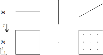
Fig. 13.2. Effect of a T-duality in the 2-direction on D1-branes at various angles in the (1,2) plane: (a) before T-duality; (b) after T-duality. The ×;s indicate a magnetic field on the D2-brane.

New connections between string theories

Starting from the toroidally compactified type I theory, we can reach either d = 10 type II theory. Simply take an odd or even number of radii to zero, while moving the D-branes and fixed planes off to infinity as the dual spacetime expands. Thus, just as for the two heterotic theories, these should be thought of as limits of a single theory. The theory has many other states as well: we can take the limit while keeping some of the D-branes in fixed positions, so that we obtain the compact theory in a state with D-branes. The simple T-duality leads only to parallel D-branes of equal dimension, but since the D-branes are dynamical we can continuously vary their configurations. We can then reach states with p-branes of different dimension as follows. Consider two D1-branes (D-strings) in the IIB theory, from dualizing in eight directions. Let one be along the 1-direction and the other be rotated to lie along the 2-direction. As illustrated in figure 13.2, a further T-duality in the 2-direction reverses Dirichlet and Neumann boundary conditions in this direction and so turns the first D-string into a D2-brane extended in the 1- and 2-directions but the second into a D0-brane. Thus these can coexist in the IIA theory. Of course T-duality leads only to states with 16 D-branes, but we understand now that this is due to the R–R flux conservation in the compact space. In a noncompact space the R–R flux can run to infinity and so any number of D-branes should be allowed.

Thus, starting from the type I theory we can reach states that look like the type IIA theory with any collection of even Dp-branes or the type IIB theory with any collection of odd Dp-branes. Of course if we start with an ordinary type II theory, T-duality will never give us open strings or D-branes, so one might imagine that there is a different type II theory in which D-branes are not allowed. This seems unlikely, however: everything we know points to the uniqueness of the theory, so we do not have such alternatives. Also, we will see in the next chapter that the inclusion of D-branes leads to a much more elegant and symmetric theory.

In summary, we are now considering a single theory, which has a state that contains no D-branes and looks like the ordinary IIA theory, a second state (T-dual to the first) that contains no D-branes and looks like the ordinary IIB theory, and a third state that contains 16 D9-branes (and an orientifold 9-plane) that looks like the type I theory. It also contains an infinite number of other states with very general configurations of D-branes.

We can now write down the supersymmetry algebra for this theory:

The spacetime supersymmetries Q_α and _α act respectively on the right- and left-movers.

The anticommutator (13.2.9b) of two right-moving supersymmetries is the same as the heterotic string anticommutator (11.6.32), containing the charge that couples to the NS–NS 2-form. The argument for the appearance of this term is the same as before: the OPE contains the right-moving momentum , which involves both ordinary momentum and winding number. Similarly, the OPE contains the left-moving momentum ∂X^μ, so the NS–NS charge appears in the left-moving anti-commutator with the opposite sign. We have added a superscript NS to distinguish this charge from the charges Q^R that couple to R–R forms. Also, we have changed conventions so that all charges are now normalized to one per unit world-volume of the respective extended object, and so the string tension (2πα′)^–1 appears explicitly. As discussed in section 11.6, is the charge carried by the fundamental string, meaning the original quantized string. Henceforth we use this term, or F-string, to distinguish it from the D1-brane.

From the argument that D-branes are BPS states, we expect the R–R charges to appear in the algebra as well, and the natural place for an R–R charge to appear is in the anticommutator of a left- and a right-moving supersymmetry. The sum on p runs over even values in the IIA theory and odd values in the IIB theory. By analogy with the NS–NS case we have included the D-brane tensions τ_p, whose values will be obtained in the next section; the factor of 1/p! offsets the sum over permutations of indices. To see that the algebra is correct, focus on a state that contains a single static D_p-brane. The nonzero charge is , where the indices run over the directions tangent to the D_p-brane. Note that

up to a possible overall sign that can be reabsorbed in the definition of ; β^⊥ is the same as in eq. (13.2.5). It then follows that the anticommutator of Q+β^⊥ with any supercharge vanishes in this state, as required by the BPS property. (In eq. (13.2.5) we included primes on the supercharges to indicate that we were working in a T-dual description to the type I theory with which we began. In writing the algebra (13.2.9) we are considering an arbitrary state with D-branes, without necessarily obtaining it from T-duality, so there are no primes.)

Incidentally, the central charge (13.2.9) is still not complete: the magnetic NS–NS charge is missing. This is not carried by D-branes or F-strings. We will discuss this further in the next chapter.

Finally, let us also explain the necessity of D-instantons, localized in time. We could try to use T-duality in the time direction, but it is not clear whether this is meaningful. Rather, consider D0-branes, whose world-lines are one-dimensional, in a space with one compact spatial dimension. For an ordinary quantized particle in a path sum description we would have to include closed paths that wind around the compact direction. Such paths are responsible for Casimir energies and other effects of compactification. Presumably we must do the same for the D0-branes as well. The shortest such winding path is a straight line in the compact spatial direction. This is localized in time and so is essentially an instanton: Casimir energies, in the path sum description, are essentially instanton effects. Further, by a T-duality in the compact dimension we obtain a D-instanton that is localized in all directions. We know from chapter 8 that the D-brane action depends on the closed string coupling as O(1/g), so the D-instanton amplitude is of order . Thus we have found an example of the enhanced nonperturbative effects that were inferred in section 9.7 from the high order behavior of string perturbation theory.

On the heterotic world-sheet there are no boundary conditions that preserve the world-sheet gauge symmetries, and there is no indication that D-branes exist. Nevertheless, we will see in the next chapter that the D-branes of the type I/II theory enable us to learn a great deal about the heterotic string as well.

13.3 The D-brane charge and action

There is no force between static BPS objects of like charge. The multi-object state is still supersymmetric and so its energy is determined only by its charge and is independent of the separations. For parallel D_p-branes, the unbroken supersymmetry (13.2.5) is the same as for a single D_p-brane.

The vanishing of the force comes about from a cancellation between attraction due to the graviton and dilaton and repulsion due to the R–R tensor. We can calculate these forces explicitly from the usual cylinder vacuum amplitude. The exchange of light NS–NS closed strings was isolated in eq. (10.8.4). Modify this expression by removing the factors for the momentum integrations in the Dirichlet directions and introducing a term for the tension of a string stretched over a separation y^µ:

with the scalar Green’s function. The Chan–Paton weight is 2 here, from the two orientations of the open string, and there is no factor of from the orientation projection because the physics is locally oriented. Due to supersymmetric cancellation in the trace, the R–R exchange amplitude is

and so the total force vanishes as expected.

The field theory calculation (8.7.25) for the dilaton–graviton potential changes only by the substitution 6 = (D – 2)/4 → 2, and so is

Thus

This satisfies the same T-duality relation as in the bosonic string. For the R–R exchange, the low-energy action is

The kinetic term is canonically normalized, so the propagator for any given component (such as the one parallel to the D-brane) is , and the field theory amplitude is

Hence

The reader can carry out a similar calculation of the force between a D-brane and an orientifold plane and show that it has an additional –(2^5–k). We deduced from the cancellation of divergences that the charge of the orientifold plane should have a factor of −(2^4−k); the extra factor of 2 in the force arises because the orientifold geometry squeezes the flux lines into half the solid angle.

The calculation of the interaction confirms our earlier deduction that D-branes carry the R–R charges. It is interesting to see how this is consistent with our earlier discussion of string vertex operators. The R–R vertex operator (12.1.14) is in the (–, –) picture, which can be used in almost all processes. On the disk, however, the total left- plus right-moving ghost number must be −2. With two or more R–R vertex operators, all can be in the (–, –) picture (with PCOs included as well), but a single vertex operator must be in either the or the picture. The (–, –) vertex operator is essentially e^–G₀ times the operator, so besides the shift in the ghost number the latter has one less power of momentum and one less Γ-matrix. The missing factor of momentum turns F into C, and the missing Γ-matrix gives the correct Lorentz representations for the potential rather than the field strength.

Dirac quantization condition

There is an important consistency check on the value of the R–R charge, which generalizes the Dirac quantization condition for magnetic monopole charge. Let us review the Dirac condition, shown in figure 13.3. Consider a magnetic charge µ_m at the origin. The integrated flux is

Because the integral over a closed surface is nonzero, we cannot write F₂ = dA₁ for any vector potential. However, we can write F₂ = dA₁ except along a Dirac string ending on the monopole. Now consider an electric charge µ_e moving in this field. Its coupling to the field produces a phase

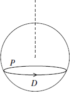
Fig. 13.3. Sphere surrounding monopole, with a Dirac string running upward. The particle path P is bounded by the lower cap D.

when the particle moves on a closed path P. The surface D spans P and does not intersect the Dirac string. Now consider the limit as the path is contracted to a small circle around the Dirac string. The phase becomes

The Dirac string must be invisible, so this phase must be 1. Equivalently, this is the condition that the phase (13.3.9) is unchanged if we instead take the surface D′ = S₂ − D spanning P in the upper hemisphere. The result is the Dirac quantization condition,

for some integer n.

A p-brane and (6 − p)-brane are sources for F_p+2 and F_8–p respectively. These two field strengths are Poincaré dual to one another, so again there is a Dirac quantization condition that must be satisfied by the product of their charges. Let us think about F_p+2 as the field strength, so that the p-brane is an electric source and the (6 − p)-brane a magnetic source. In nine dimensions a (6 − p)-dimensional object is surrounded by a (p + 2)-sphere, so by analogy to the magnetic flux (13.3.8),

One can then repeat the same argument. For example, let the p-brane be extended in the directions 4 ≤ μ ≤ p + 3 and the (6 − p)-brane in the directions p + 4 ≤ μ ≤ 9. The system essentially reduces to the three-dimensional situation of figure 13.3 in the directions µ = 1, 2, 3, and the charges must satisfy

Remarkably, the charges (13.3.7), arrived at in an entirely different way, satisfy this relation with the minimum quantum n = 1.

D-brane actions

The coupling of a D-brane to NS–NS closed string fields is the same Dirac–Born–Infeld action as in the bosonic string,

where G_ab and B_ab are the components of the spacetime NS–NS fields parallel to the brane and F_ab is the gauge field living on the brane. The argument leading to this form is exactly as in the bosonic case, section 8.7. Recall that for n D-branes at small separation, where the strings stretched between them are light enough to be included in the low energy action, the collective coordinates Xµ(ξ), gauge fields A_a(ξ), and their fermionic partners λ(ξ) all become n × n matrices. The trace in the action is in this n × n space. In addition there is a term

in the potential. As discussed in chapter 8, the effect of this potential is that in the flat directions the collective coordinates become diagonal. They can then be interpreted as n ordinary collective coordinates for n objects. At small separation the full matrix dynamics is crucial, as we will see.

The coupling to the R–R background also includes corrections involving the gauge field on the brane. Like the Born–Infeld action, these can be deduced via T-duality. Consider, as an example, a 1-brane in the (1,2) plane. The action is

Under a T-duality in the 2-direction this becomes

We have used the T-transformation of the C fields, eq. (13.1.5). A D-brane at an angle is T-dual to one with a magnetic field, as in figure 13.2. We are not keeping track of the normalization but one could, with the result µ_p = µ_p–1/2πα′^1/2 in agreement with the explicit calculation. The generalization of (13.3.17) to an arbitrary configuration, and to multiple D-branes, gives the Chern–Simons-like result

The expansion of the integrand (13.3.18) involves forms of various rank; the integral picks out precisely the terms that are proportional to the volume form of the p-brane world-volume. There are similar couplings with the spacetime curvature in addition to the field strength; these can be obtained from a string calculation.

Thus far we have given only the action for the bosonic fields on the brane. For the leading fluctuations around a flat D-brane in flat spacetime the fermionic action is of the usual Dirac form

The full nonlinear supersymmetric form is left to the references.

Coupling constants

The ratio of the F-string tension to the D-string tension is

Up to now there has been no natural convention for defining the additive normalization of the dilaton field or the multiplicative normalization of the closed string coupling g = e^Φ. The dimensionless ratio (13.3.20) is proportional to the closed string coupling, and it turns out to be very convenient to take it as the definition of the coupling,

Then the gravitational coupling is

and the D-brane tension is

Also, the constant appearing in the low energy actions of section 12.1 is

this differs from the physically measured κ because the latter depends on the dilaton background.

Expanding the action (13.3.14) gives the coupling of the Yang–Mills theory on the D_p-brane,

Notice that for p = 3 this coupling is dimensionless, as expected in a (3 + 1)-dimensional gauge theory. For p < 3 the coupling has units of length to a negative power, and for p > 3 length to a positive power.

We now wish to obtain the relation among κ, g_YM, and α′ in the type I theory. We cannot quite identify g_Dp for p = 9 with g_YM, because the former has been obtained in a locally oriented theory and there are some additional factors of 2 in the type I case. Rather than repeat the string calculation we will make a more roundabout but possibly instructive argument using T-duality.

First, we should note that the coupling (13.3.25) is for the U(n) gauge theory of coincident branes in the oriented theory: it appears in the form

where the trace is in the n × n fundamental representation. Now let us consider moving the branes to an orientifold plane so that the gauge symmetry is enlarged to SO(2n). An SU(n) generator t is embedded in SO(2n) as

because the orientation projection reverses the order of the Chan–Paton factors and the sign of the gauge field. Comparing the low energy actions gives

and so .

Now consider the type I theory compactified on a k-torus with all radii equal to R. The couplings in the lower-dimensional SO(32) theory are related to those in the type I theory by

In the T-dual picture, the bulk theory is of type II and the gauge fields live on a D(p – k)-brane, and

The dimensional reduction for has an extra factor of 2 because the compact space is an orientifold, its volume halved. The gauge coupling is independent of the volume because the fields are localized on the D-brane. Combining these results with the relations (13.3.22) and (13.3.25) gives, independent of k, the type I relation

As one final remark, the Born–Infeld form for the gauge action applies by T-duality to the type I theory:

whose normalization is fixed by the quadratic term in F. In the previous chapter we obtained the tree-level string correction (12.4.28) to the type I effective action. If the gauge field lies in an Abelian subgroup, the tensor structure simplifies to

This is indeed the quartic term in the expansion of the Born–Infeld action, as one finds by using

with . The trace here is on the Lorentz indices, and tr(x^2k+1) = 0 for antisymmetric x. Note that only when the gauge field can be diagonalized can we give a geometric interpretation to the T-dual configuration and so derive the Born–Infeld form.

13.4 D-brane interactions: statics

Many interesting new issues arise with D-branes that are not parallel, or are of different dimensions. In this section we focus on static questions. The first of these concerns the breaking of supersymmetry. Let us consider a Dp-brane and a Dp′-brane, which we take first to be aligned along the coordinate axes. That is, we can partition the spacetime directions µ into two sets S_D and S_N according to whether the coordinate X^µ has Dirichlet or Neumann boundary conditions on the first D-brane, and similarly into two sets and depending on the alignment of the second D-brane. The DD coordinates are S_D ∩ , the ND coordinates are S_N ∩ , and so on.

The first D-brane leaves unbroken the supersymmetries

Similarly the second D-brane leaves unbroken

The complete state is invariant only under supersymmetries that are of both forms (13.4.1) and (13.4.2). These are in one-to-one correspondence with those spinors left invariant by β^{⊥ –1}β^⊥′. The operator β^⊥–1β^⊥′ is a reflection in the DN and ND directions. Let us denote the total number of DN and ND directions ≠ND. Since p – p′ is always even the number ≠ND = 2j is also even. We can then pair these dimensions and write (β^⊥)^–1β^⊥′ as a product of rotations by π,

In a spinor representation, each exp(iπJ) has eigenvalues ±i, so there will be unbroken supersymmetries only if j is even and so is a multiple of 4. In this case there are 8 unbroken supersymmetries, one quarter of the original 32. Note that T-duality switches NN↔DD and ND↔DN and so leaves invariant. When = 0, then (β^⊥)^–1β^⊥′ = 1 identically and there are 16 unbroken supersymmetries. This is the same as for the original type I theory, to which it is T-dual.

An open string can have both ends on the same D-brane or one on each. The p-p and p′-p′ spectra are the same as obtained before by T-duality from the type I string, but the p-p′ strings are new. Each of the four possible boundary conditions can be written with the doubling trick

in terms of one of two mode expansions,

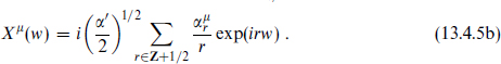
The periodic expansion (13.4.5a) describes NN strings for

and DD strings for

The antiperiodic expansion (13.4.5b) similarly defines DN and ND strings, with . For ψ^µ, the periodicity in the R sector is the same as for X^µ because T_F is periodic. In the NS sector it is the opposite.

The string zero-point energy is zero in the R sector as always, because bosons and fermions with the same periodicity cancel. In the NS sector it is

The oscillators can raise the level in half-integer units, so only for a multiple of 4 is degeneracy between the R and NS sectors possible. This agrees with the analysis above: the = 2 and = 6 systems cannot be supersymmetric. Later we will see that there are supersymmetric bound states when = 2, but their description is rather different.

Branes at general angles

It is interesting to consider the case of D-branes at general angles to one another. To be specific consider two D4-branes. Let both initially be extended in the (2,4,6,8)-directions, and separated by some distance y₁ in the 1-direction. Now rotate one of them by an angle ₁ in the (2, 3) plane, ₂ in the (4, 5) plane, and so on; call this rotation ρ. The supersymmetry unbroken by the rotated 4-brane is

Supersymmetries left unbroken by both branes then correspond to spinors left invariant by

In the usual s-basis the eigenvalues of ρ² are

In the 16 the run over all 16 combinations of ±1s; each combination such that the phase (13.4.11) is 1 gives an unbroken supersymmetry. There are many possibilities — for example:

• For generic _a there are no unbroken supersymmetries.

• For angles ₁ + ₂ + ₃ + ₄ = 0 mod 2π (but otherwise generic) there are two unbroken supersymmetries, namely those with s₁ = s₂ = s₃ = s₄. The rotated D4-brane breaks seven-eighths of the supersymmetry of the first.

• For ₁ + ₂ + ₃ = ₄ = 0 mod 2π there are four unbroken supersymmetries.

• For ₁ + ₂ + ₃ + ₄ = 0 mod 2π there are four unbroken supersymmetries.

• For ₁ + ₂ = ₃ = ₄ = 0 mod 2π there are eight unbroken supersymmetries.

Also, when k angles are π/2 and the rest are zero this reduces to the earlier analysis with = 2k.

For later reference let us also describe these results as follows. Join the coordinates into complex pairs, Z¹ = X² + iX³ and so on, with the conjugate denoted Z^ā. Then ρ takes Z^a to exp(i_a)Z^a. The SO(8) rotation group on the transverse dimensions has a U(4) subgroup that preserves the complex structure. That is, it rotates Z′^a = U^abZ^b, whereas a general SO(8) rotation would mix in as well. The rotation ρ in particular is the U(4) matrix

When ₁ + ₂ + ₃ + ₄ = 0 mod 2π, which is the condition for two supersymmetries to be unbroken, the determinant of ρ is 1 and so it actually lies in the SU(4) subgroup of U(4). Then we can summarize the above by saying that a general U(4) rotation breaks all the supersymmetry, an SU(4) rotation breaks seven-eighths, an SU(3) or SU(2) × SU(2) rotation breaks three-quarters, and an SU(2) rotation half. Further, if we consider several branes, so that in general the rotations ρi cannot be simultaneously diagonalized, then as long as all of them lie within a given subgroup the number of unbroken supersymmetries is as above.

Now let us calculate the force between these rotated branes. The cylinder graph involves traces over the p-p′ strings, so we need to generalize the mode expansion to the rotated case. Letting the σ¹ = 0 endpoint be on the unrotated brane and the σ¹ = π endpoint on the rotated brane, it follows that the boundary conditions are

These are satisfied by

where w = σ¹ + iσ². This implies the mode expansion

with ν_a = _a/π. The modes are linearly independent.

The partition function for one such complex scalar is

with q = exp(− 2πt), 0 < < π (else subtract the integer part of /π), and

The definitions and properties of theta functions are collected in section 7.2, but we reproduce here the results that will be most useful:

where z = exp(2πiν). Similarly in each of the sectors of the fermionic path integral one replaces the (it) that appears for parallel D-branes with⁴

The full fermionic partition function is

generalizing the earlier (it). By a generalization of the abstruse identity (7.2.41), the fermionic partition function can be rewritten

where

This identity has a simple physical origin. If we refermionize, writing the theory in terms of the free fields θ_α as in eq. (12.6.24), we get the form (13.4.21) directly. In particular, the exp(±i′_a) are the eigenvalues of ρ in the spinor 8 of SO(8).

Collecting all factors, the potential is

Note that for nonzero angles the stretched strings are confined near the point of closest approach of the two 4-branes. The function ₁₁(ν, it) is odd in ν and so vanishes when ν = 0. If any of the _a vanish the denominator has a zero. This is because the 4-branes become parallel in one direction and the strings are then free to move in that direction. One must replace

This gives the usual factors for a noncompact direction, L being the length of the spatial box. Taking ₄ → 0 so the 4-branes both run in the 8-direction, one can T-dualize in this direction to get a pair of 3-branes with relative rotations in three planes. The fermionic partition function is unaffected, while the factors (13.4.24) are instead replaced by

allowing for the possibility of a separation in the (8,9) plane. Taking the T-dual in the 9-direction instead one obtains 5-branes that are separated in the 1-direction, extended in the (8,9)-directions, and with relative rotations in the other three planes. The effect is an additional factor of L₉(8π²α′t)^−1/2. The extension to other p is straightforward.

If instead any of the vanishes, the potential is zero. The reason is that there is unbroken supersymmetry: the phases (13.4.11) include exp(±2). Curiously this covers only eight of the sixteen phases (13.4.11), so that if some phases (13.4.11) are unity but not those of the form exp(±2i), then supersymmetry is unbroken but the potential is nonzero. This is an exception to the usual rule that the vacuum loop amplitudes vanish by Bose–Fermi cancellation. The rotated D-branes leave only two supersymmetries unbroken, so that BPS multiplets of open strings contain a single bosonic or fermionic state.

The potential is a complicated function of position, but at long distance it simplifies. The exponential factor in the integral (13.4.23) forces t to be small, and then the -functions simplify,

by using the modular transformation of ₁₁. The t-integral then gives a power of the separation y₁. The result agrees with the low energy field theory calculation, including the angular factor. For 4-branes with all _a nonzero the potential grows linearly with y₁ at large distance, for 3-branes with all _a nonzero it falls as 1/y₁, and so on.

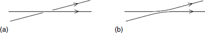
Fig. 13.4. (a) D-branes at relative angle. (b) Lower energy configuration.

In nonsupersymmetric configurations a tachyon can appear. For simplicity let only ₁ be nonzero, with 0 ≤ ₁ ≤ π. The NS ground state energy is −(1/2) + (₁/2π), and the first excited state , which survives the GSO projection, has weight −₁/2π. Including the energy from tension, the lightest state has

This is negative if the separation is small enough. A special case is ₁ = π, when the 4-branes are antiparallel rather than parallel. The NS–NS and R–R exchanges are then both attractive, and below the critical separation = 8π²α′ the cylinder amplitude diverges as t → ∞. This is where the tachyon appears — evidently it represents D4-brane/anti-D4-brane annihilation. Even when the D-branes are nearly parallel they can lower their energy by reconnecting as in figure 13.4(b), and this is the origin of the instability. This is one example where the tachyon has a simple physical interpretation and we can see that the decay has no end: the reconnected strings move apart indefinitely. On the other hand, for the same instability but with the strings wound on a two-torus there is a lower bound to the energy.

13.5 D-brane interactions: dynamics

D-brane scattering

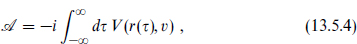
For parallel static D-branes the potential energy is zero, but if they are in relative motion all supersymmetry is broken and there is a velocitydependent force. This can be obtained by an analytic continuation of the static potential for rotated branes. Consider the case that only ₁ is nonzero, so the rotated brane satisfies X³ = X²tan₁. Analytically continue X² → iX′⁰ and let ₁ = –iu, with u > 0. Then

which describes a D-brane moving with constant velocity. Continue also X⁰ → −iX′² to eliminate the spurious extra time coordinate. The interaction amplitude (13.4.23) between the D-branes becomes

where we have extended the result to general p by using T-duality.⁵ It is also useful to give the modular transformation

We can write this as an integral over the world-line,

where

and

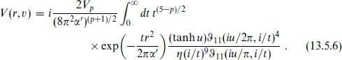
The interaction has a number of interesting properties. The first is that as v → 0 (so that u → 0), it vanishes as v⁴ from the zeros of the theta functions. We expect only even powers of v by time-reversal invariance. The vanishing of the v² interaction, like the vanishing of the static interaction, is a consequence of supersymmetry. The low energy field theory of the D-branes is a U(1) × U(1) supersymmetric gauge theory with 16 supersymmetries. What we are calculating is a correction to the effective action from integrating out massive states, strings stretched between the D-branes. The vanishing of the v² term is then consistent with the assertion in section B.6 that with 16 supersymmetries corrections to the kinetic term are forbidden — the moduli space is flat. If we had instead taken ₃ = ₄ = π/2 so that = 4, there would only be two zeros in the numerator and thus a v² interaction. This is consistent with the result that corrections to the kinetic term are allowed when there are eight unbroken supersymmetries.

The interaction (13.5.6) is in general a complicated function of the separation, but in an expansion in powers of the velocity the leading O(v⁴) term is simple,

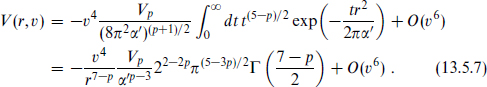
At long distances this is in agreement with low energy supergravity. It is also the leading behavior if we expand in powers of 1/r rather than v.

In general the behavior of V(r, v) as r → 0 is quite different from the behavior as r → ∞. The r-dependence of the integral (13.5.6) arises from the factor exp(−tr²/2πα′), so that t ≈ 2πα′/r² governs the behavior at given r. Large r corresponds to small t, where the asymptotic behavior is given by tree-level exchange of light closed strings — hence the agreement with classical supergravity. Small r corresponds to large t, where the asymptotic behavior is given by a loop of the light open strings. The cross-over is at r² ∼ 2πα′. This is as we expect: string theory modifies gravity at distances below the string scale.

This simple r-dependence of the v⁴ term is another consequence of supersymmetry. The fact that this term is singular as r → 0 might seem to conflict with the assertion that string theory provides a short-distance cutoff. However, one must look more carefully. To obtain the small-r behavior of the scattering amplitude (13.5.6), take the large-t limit without expanding in v to obtain

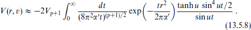
Since t ≈ 2πα′/r² and v ≈ u, the arguments of the sines are ut ≈ 2πα′v/r². No matter how small v is the v⁴ term will cease to dominate at small enough r. The oscillations of the integrand then smooth the small-r behavior on a scale ut ≈ 1. The effective scale probed by the scattering is

A small-velocity D-brane probe is thus sensitive to distances shorter than the string scale. This is in contrast to the behavior we have seen in string scattering at weak coupling, but fits nicely with the understanding of strongly coupled strings in the next chapter.

Let us expand on this result. A slower D-brane probes shorter distances, but the scattering process takes longer, δt ≈ r/v. Then

This is a suggestion for a new uncertainty relation involving only the coordinates. It is another indication of ‘noncommutative geometry,’ perhaps connected with the promotion of D-brane collective coordinates to matrices.

For a pointlike D0-brane probe there is a minimum distance that can be measured by scattering. The wavepacket in which it is prepared satisfies

The combined uncertainties (13.5.9) and (13.5.11) are minimized by v ≈ g^2/3, for which

We will see the significance of this scale in the next chapter.

D0-brane quantum mechanics

The nonrelativistic effective Lagrangian for n D0-branes is

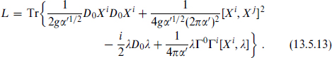
The first term is the usual nonrelativistic kinetic energy with m = τ₀ = 1/gα′^1/2, dropping the constant rest mass nτ₀. The coefficients of the other terms are most easily obtained by T-duality from the ten-dimensional super-Yang-Mills action (B.6.13), with Aⁱ → Xⁱ/2πα′. We have taken a basis in which the fermionic field λ is Hermitean, and rescaled λ to obtain a canonical kinetic term. The index i runs over the nine spatial dimensions. The gauge field A⁰ has no kinetic term but remains in the covariant derivatives. It couples to the U(n) charges, so its equation of motion amounts to the constraint that only U(n)-invariant states are allowed. Only terms with at most two powers of the velocity have been kept, not the full Born–Infeld action.

The Hamiltonian is

Note that the potential is positive because [Xⁱ, X^j] is anti-Hermitean. The canonical momentum, like the coordinate, is a matrix,

Now we define

so that also p_i = p_Yi/g^1/3 α′^1/2. The Hamiltonian becomes

The parameters g and α′ now appear only in the overall normalization. It follows that the wavefunctions are independent of the parameters when expressed in terms of the variables Yⁱ. In terms of the original coordinates Xⁱ their characteristic size scales as g^1/3 α′^1/2, the same scale (13.5.12) found above. The energies scale as g^1/3 /α′^1/2 from the overall normalization of H, and the characteristic time scale as the inverse of this, so we find again the relation (13.5.10).

Recall from the discussion of D-brane scattering that at distances less than the string scale only the lightest open string states (those which become massless when the D-branes are coincident) contribute. In this regime the cylinder amplitude reduces to a loop amplitude in the low energy field theory (13.5.13).

The = 4 system

Another low energy action with many applications is that for a Dp-brane and D_p′-brane with relative = 4. There are three kinds of light strings: p-p, p-p′, and p′-p′, with ends on the respective D-branes. We will consider explicitly the case p = 5 and p′ = 9, where we can take advantage of the SO(5, 1) × SO(4) spacetime symmetry; all other cases are related to this by T-duality.

The 5-5 and 9-9 strings are the same as those that arise on a single D-brane. The new feature is the 5-9 strings; let us study their massless spectrum. The NS zero-point energy is zero. The moding of the fermions differs from that of the bosons by , so there are four periodic world-sheet fermions ψ^m, namely those in the ND directions m = 6, 7, 8, 9. The four zero modes then generate 2^4/2 = 4 degenerate ground states, which we label by their spins in the (6, 7) and (8, 9) planes,

with s₃, s₄ taking values ±. Now we need to impose the GSO projection. This was defined in eq. (10.2.22) in terms of s_a, so that with the extra sign from the ghosts it is

In terms of the symmetries, the four states (13.5.18) are invariant under SO(5, 1) and form spinors 2 + 2′ of the ‘internal’ SO(4), and only the 2 survives the GSO projection. In the R sector, of the transverse fermions ψⁱ only those with i = 2, 3, 4, 5 are periodic, so there are again four ground states

The GSO projection does not have a extra sign in the R sector so it requires s₁ = − s₂. The surviving spinors are invariant under the internal SO(4) and form a 2′ of the SO(4) little group of a massless particle.

The system has six-dimensional Lorentz invariance and eight unbroken supersymmetries, so we can classify it by d = 6, N = 1 supersymmetry (section B.7). The massless content of the 5-9 spectrum amounts to half of a hypermultiplet. The other half comes from strings of opposite orientation, 9-5. The action is fully determined by supersymmetry and the charges; we write the bosonic part:

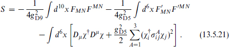
The integrals run respectively over the 9-brane and the 5-brane, with M = 0, ..., 9, µ = 0, ..., 5, and m = 6, ..., 9. The covariant derivative is with A_µ and the 9-brane and 5-brane gauge fields. The field χ_i is a doublet describing the hypermultiplet scalars. The 5-9 strings have one endpoint on each D-brane so χ carries charges +1 and −1 under the respective symmetries. The gauge couplings g_Dp were given in eq. (13.3.25). We are using a condensed notation,

The massless 5-5 (and also 9-9) strings separate into d = 6, N = 1 vector and hypermultiplets. The final potential term is the 5-5 D-term required by the supersymmetry. One might have expected a 9-9 D-term as well by T-duality, but this is inversely proportional to the volume of the D9-brane in the (6,7,8,9)-directions, which we have taken to be infinite.

Under T-dualities in any of the ND directions, one obtains (p, p′) = (8, 6), (7, 7), (6, 8), or (5, 9), but the intersection of the branes remains (5+ 1)-dimensional and the p-p′ strings live on the intersection with action (13.5.21). T-dualities in r NN directions give (p, p′) = (9 − r, 5 − r). The vector components in the dualized directions become collective coordinates as usual,

The term D_iχ^†Dⁱχ then becomes

This just reflects the fact that when the (9 − r)-brane and (5 − r)-brane are separated, the strings stretched between them become massive.

The action for several branes of each type is given by the non-Abelian extension.

13.6 D-brane interactions: bound states

Bound states of D-branes with strings and with each other, and supersymmetric bound states in particular, present a number of interesting dynamical problems. Further, these bound states will play an important role in the next chapter in our attempts to deduce the strongly coupled behavior of string theory.

FD bound states

The first case we consider is a state with p F-strings and q D-strings in the IIB theory, all at rest and aligned along the 1-direction. For a state with these charges, the supersymmetry algebra (13.2.9) becomes

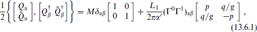
where L₁ is the length of the system. The eigenvalues of Γ⁰Γ¹ are ±1, so those of the right-hand side are

The left-hand side of the algebra is positive — its expectation value in any state is a matrix with positive eigenvalues. This implies a BPS bound on the total energy per unit length,

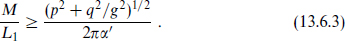
This inequality is saturated by the F-string, which has (p, q) = (1, 0), and by the D-string, with (p, q) = (0, 1).

For one F-string and one D-string, the total energy per unit length is

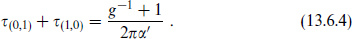
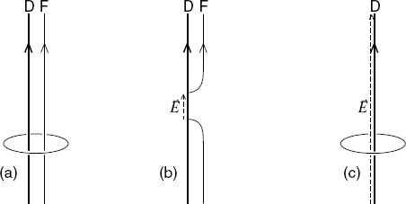
Fig. 13.5. (a) Parallel D-string and F-string. The loop signifies a 7-sphere surrounding the strings. (b) The F-string breaks, its ends attaching to the D-string. (c) Final state: D-string with flux.

This exceeds the BPS bound

and so this configuration is not supersymmetric. One can also see this directly. The F-string is invariant under supersymmetries satisfying

and no linear combination of these is of the form Q_α + (β┴)_α preserved by the D-string (note that β┴Γ⁰Γ¹ = Γ⁰Γ¹β┴).

However, the system can lower its energy as shown in figure 13.5. The F-string breaks, with its endpoints attached to the D-string. The endpoints can then move off to infinity, leaving only the D-string behind. This cannot be the whole story because the F-string carries the NS–NS 2-form charge, as measured by the integral of ∗H over the 7-sphere in the figure: this flux must still be nonzero in the final configuration. This comes about because the F-string endpoints are charged under the D-string gauge field, so an electric flux runs between them. This flux remains in the end. Further, from the D-string action

one sees that B_µν has a source proportional to the invariant electric flux on the D-string.

The simplest way to see that the resulting state is supersymmetric is via T-duality along the 1-direction. The D1-brane becomes a D0-brane. The electric field is T-dual to a velocity, 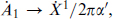so the T-dual state is a D0-brane moving with constant velocity. This is invariant under the same number of supersymmetries as a D-brane at rest, namely the Lorentz boost of those supersymmetries. The boosted supersymmetries are linear combinations of the unbroken and broken supersymmetries of the D0-brane at rest. All of this carries over by T-duality to the D1–F1 system. We leave it as an exercise to verify that the tension takes the BPS value.

The F-string ‘dissolves’ in the D-string, leaving flux behind. For separated D- and F-strings there is an attractive force at long distance, a consequence of the lack of supersymmetry. One might have expected a more standard description of the bound state in terms of the F-string moving in this potential well. However, this description breaks down at short distance; happily, the D-brane effective theory gives a simple alternative description. Note that the bound state is quite deep: the binding tension

is almost the total tension of the F-string.

String theory with a constant open string field strength has a simple world-sheet description. The variation of the world-sheet action includes a surface term

implying the linear boundary condition

This can also be seen from the T-dual relation to the moving D-brane.

All of the above extends immediately to p F-strings and one D-string forming a supersymmetric (p, 1) bound state. The general case of p F-strings and q D-strings is more complicated because the gauge dynamics on the D-strings is non-Abelian. A two-dimensional gauge coupling has units of inverse length-squared; we found the precise value in eq. (13.3.25). For dynamics on length scale l the effective dimensionless coupling is gl²/2πα′. No matter how weak the underlying string coupling g, the D-string dynamics at long distances is strongly coupled — this is a relevant coupling. The theory cannot then be solved directly, but it has been shown by indirect means that there is a bound string saturating the BPS bound for all (p, q) such that p and q are relatively prime. We will sketch the argument and leave the details to the references.

Focus for example on two D-strings and one F-string. There is a state with a separated (1, 1) bound state and (0, 1) D-string. The tension

exceeds the BPS bound

The electric flux is on the first D-brane, so as a U(2) matrix this is proportional to

We have separated this into U(1) and SU(2) pieces. When we bring the two D-strings together, the SU(2) field becomes strongly coupled as we have explained but the U(1) part remains free. The U(1) flux is then unaffected by the dynamics, and in particular there are no charged fields that might screen it. However, if the SU(2) part is screened by the massless fields on the D-strings, then the total energy in the flux (which is proportional to the trace of the square of the matrix) is reduced by a factor of 2, from (13.6.11) to the BPS value (13.6.12).

That this does happen has been shown as follows. Focus on four of the 16 supersymmetries, forming the equivalent of d = 4, N = 1 super-symmetry. The six scalars X^{4,..., 9} can be written as three chiral superfields Φ_i, with the potential coming from a superpotential Tr(Φ₁[Φ₂, Φ₃]). Now change the problem, adding to the superpotential a mass term,

This is an example of a general strategy for finding supersymmetric bound states: the D-string is a BPS state even under the reduced supersymmetry algebra. Its mass is then determined by the algebra and cannot depend on the parameter m. By now increasing m we can reduce the effective dimensionless coupling g/2πα′m² to a value where the system becomes weakly coupled. It can then be shown that the SU(2) system has a supersymmetric ground state.

The same argument goes through for all relatively prime p and q. When these are not relatively prime, (p, q) = (kp, kq) and the system is only marginally unstable against falling apart into k subsystems. The dynamics is then quite different, and there is believed to be no bound string in this case. The bound string formed from p F-strings and q D-strings is called a (p, q)-string (as opposed to a p-p′ string, which is an open string whose endpoints move on Dp- and Dp′-branes).

D0–Dp BPS bound

For a system with the charges of a D0-brane and a Dp-brane extended in the (1, ..., p)-directions, the supersymmetry algebra becomes

where

We have wrapped the Dp-brane on a torus of volume V_p so that its mass will be finite. The positivity of the left-hand side implies that

For p a multiple of 4, β is Hermitean and β² = 1 by the same argument as in eq. (13.4.3). The BPS bound is then

For p = 4k + 2, β is anti-Hermitean, β² = −1, and the BPS bound is

These bounds are consistent with our earlier results on supersymmetry breaking, noting that = p. For p = 4k, a separated 0-brane and p-brane saturate the BPS bound (13.6.18), agreeing with the earlier conclusion that they leave some supersymmetry unbroken. For p = 4k + 2 they do not saturate the bound and so cannot be in a BPS state, as found before. The reader can extend the analysis of the BPS bound to general values of p and p′.

D0–D0 bound states

The BPS bound for the quantum numbers of two 0-branes is 2τ₀, so any bound state will be at the lower edge of the continuous spectrum of two-body states. Nevertheless there is a well-defined, and as it turns out very important, question as to whether a normalizable state of energy 2τ₀ exists.

Let us first look at an easier problem. Compactify the 9-direction and add one unit of compact momentum, p₉ = 1/R. In a two-body state this momentum must be carried by one 0-brane or the other for minimum total energy

For a bound state of mass 2τ₀, on the other hand, the minimum energy is

a finite distance below the continuum states. The reader may note some resemblance between these energies and the earlier (13.6.11) and (13.6.12). In fact the two systems are T-dual to one another. Taking the T-dual along the 9-direction, the D0-branes become D1-branes and the unit of momentum becomes a unit of fundamental string winding to give the (1, 2) system, now at finite radius R′ = α′/R. Quantizing the (1, 2) string wrapped on a circle gives the 2⁸ states of an ultrashort BPS multiplet. In terms of the previous analysis, the SU(2) part has a unique ground state in finite volume while the zero modes of the 16 components of the U(1) gaugino generate 2⁸ states. The earlier analysis is valid for the T-dual radius R′ large, but having found an ultrashort multiplet we know that it must saturate the BPS bound exactly — its mass is determined by its charges and cannot depend on R. Similarly for n D-branes with m units of compact momentum, when m and n are relatively prime there is an ultrashort multiplet of bound states.

Now let us try to take R → ∞ in order to return to the earlier problem. Having found that a bound state exists at any finite radius, it is natural to suppose that it persists in the limit. Since for any n we can choose a relatively prime m, it appears that there is one ultrashort bound state multiplet for any number of D0-branes. However, it is a logical possibility that the size of these states grows with R such that the states becomes nonnormalizable in the limit. To show that the bound states actually exist requires a difficult analysis, which has been carried out fully only for n = 2.

D0-D2 bound states

Here the BPS bound (13.6.19) puts any bound state discretely below the continuum. One can see hints of a bound state: the long-distance force is attractive, and for a coincident 0-brane and 2-brane the NS 0-2 string has a negative zero-point energy (13.4.8) and so a tachyon (which survives the GSO projection), indicating instability towards something. We cannot follow the tachyonic instability directly, but there is a simple alternative description of where it must end up.

Let us compactify the 1- and 2-directions and take the T-dual only in the first, so that the 0-brane becomes a D-string wrapped in the 1-direction and the 2-brane becomes a D-string wrapped in the 2-direction. Now there is an obvious state with the same charges and lower energy, a single D-string running at an angle to wrap once in each direction. A single wrapped D-string is a BPS state (an ultrashort multiplet to be precise). Now use T-duality to return to the original description. As in figure 13.2, this will be a D2-brane with a nonzero magnetic field, such that

We can also check that this state has the correct R−R charges. Expanding out the Chern–Simons action (13.3.18) gives

Thus the magnetic field induces a D0-brane charge on the D2-branes, and the normalizations are consistent with µ₀ = 4π²α′µ₂.

The D0-brane dissolves in the D2-brane, turning into flux. The reader may note several parallels with the discussion of a D-string and an F-string, and wonder whether the systems are equivalent. In fact, they are not related to one other by T-duality or any other symmetry visible in string perturbation theory, but we will see in the next chapter that they are related by nonperturbative dualities.

The analysis extends directly to n D2-branes and m D0-branes: there is a single ultrashort multiplet of bound states.

D0–D4 bound states

As with the D0–D0 case, the BPS bound (13.6.18) implies that any bound state is marginally stable. We can proceed as before, first compactifying another dimension and adding a unit of momentum so that the bound state lies below the continuum. The low energy D0–D4 action is as discussed at the end of the previous section. Again it is an interacting theory, with a coupling that becomes large at low energy, but again the existence of supersymmetric bound states can be established by deforming the Hamiltonian; the details are left to the references. A difference from the D0–D0 case is that these bound states are invariant only under one-quarter of the original supersymmetries, the intersection of the supersymmetries of the 0-brane and of the 4-brane. The bound states then lie in a short (but not ultrashort) multiplet of 2¹² states. It is useful to imagine that the D4-brane is wound on a finite but large torus. In this limit the massless 4-4 strings are essentially decoupled from the 0-4 and 0-0 strings. The 16 zero modes of the massless 4-4 fermion then generate 2⁸ ground states delocalized on the D4-brane. The fermion in the 0-4 hypermultiplet has eight real components (the smallest spinor in six dimensions) and their zero modes generate 2⁴ ground states localized on the D0-brane. The tensor product gives the 2¹² states.

For two D0-branes and one D4-brane, one gets the correct count as follows. We can have the two D0-branes bound to the D4-brane independently of one another; for a large D4-brane their interactions can be neglected. Each D0-brane has 2⁴ states as noted above, eight bosonic and eight fermionic. Now count the number of ways two D0-branes can be put into these states: there are eight states with both D0-branes in the same (bosonic) state and × 8 × 7 states with the D-branes in different bosonic states, for a total of × 8 × 9 states. There are also × 8 × 7 states with the D0-branes in different fermionic states and 8 × 8 with one in a bosonic state and one a fermionic state. Summing and tensoring with the 2⁸ D4-brane states gives 2¹⁵ states. However, we could also imagine the two D0-branes first forming a D0–D0 bound state. The SU(2) dynamics decouples and the resulting U(1) dynamics is essentially the same as that of a single D0-brane. This bound state can then bind to the D4-brane, giving 2⁴⁺⁸ states as for a single D0-brane. The total number is 9 × 2¹².

This counting extends to n D0-branes and one D4-brane. The degeneracy D_n is given by the generating function

The term k in the product comes from bound states of k D0-branes which are then bound to the D4-brane. For each k there are eight bosonic states and eight fermionic states, and the expression (13.6.24) is then the product of the partition functions for all species. The coefficient of q² in its expansion is indeed 9 × 2¹². This proliferation of bound states is in contrast to the single ultrashort multiplet for n D0-branes and one D2-brane. The difference is that all the latter states are spread over the D2-brane, whereas the D0–D4 bound states are localized.

By T-duality the above system is converted into one D0-brane and n D4-branes, so the number of bound states of the latter is the same D_n. For m D0-branes and n D4-branes one gets the correct answer by the following argument. The equality of the degeneracy for one D0-brane and n D4-branes with that for n D0-branes and one D4-brane suggests that the systems are really the same — that in the former case we can somehow picture the D0-brane bound to n D4-branes as separating into n ‘fractional branes,’ each of which can then bind to each other in all combinations as in the earlier case. Then m D0-branes separate into mn fractional branes. The degeneracy would then be D_mn, defined as in eq. (13.6.24). This is apparently correct, but the justification is not simple.

D-branes as instantons

The D0–D4 system is interesting in other ways. Consider its scalar potential

as at the end of the previous section. The second term by itself has two branches of zeros,

and

The first of these, where the hypermultiplet scalars are nonzero, is known as a Higgs branch. The second, where the vector multiplet scalars are nonzero, is known as a Coulomb branch. In the present case the first term in the potential, the D-term, eliminates the Higgs branch. The condition

implies that χ = 0. For example, if there were a nonzero solution we could by an SU(2) rotation make only the upper component nonzero, and then D³ is nonzero. However, for two D4-branes χ acquires a D4-brane index a = 1, 2 and the D-term condition is

This now is solved by

for any v, or more generally

for any constant v and unitary U. Further, U can be taken to lie in SU(2) by absorbing its phase into v, and the latter can then be made real by a 4–4 U(1) gauge rotation.

The Coulomb branch has an obvious physical interpretation, corresponding to the separation of the D0- and D4-brane in the directions transverse to the latter. But what of the Higgs branch?

Recall that non-Abelian gauge theories in four Euclidean dimensions have classical solutions, instantons, that are localized in all four dimensions. Their distinguishing property is that the field strength is self-dual or anti-self-dual,

so that the Bianchi identity implies the field equations. Because the classical theory is scale-invariant, the characteristic size of the configuration is undetermined — there is a family of solutions parameterized by scale size ρ. The U(n) gauge theory on coincident D4-branes is five-dimensional, so a configuration that looks like an instanton in the four spatial dimensions and is independent of time is a static classical solution, a soliton.

This soliton has many properties in common with the D0-brane bound to the D4-branes. First, it is a BPS state, breaking half of the supersymmetries of the D4-branes. The supersymmetry variation of the gaugino is

Here the nonzero terms involve the components of Γ^MN in the spatial directions of the D4-brane. These are then generators of the SO(4) = SU(2) × SU(2) rotation group. The self-duality relation (13.6.32) amounts to the statement that only the generators of the first or second SU(2) appear in the variation. The ten-dimensional spinor ζ decomposes into

under SO(5, 1) × SU(2) × SU(2), so half the components are invariant under each SU(2) and half the supersymmetry variations (13.6.33) are zero. Second, it carries the same R–R charge as the D0-brane. Expanding the Chern–Simons action (13.3.18) gives the term

The topological charge of the instanton is

so the total coupling to a constant C₁ is (4π²α′)²µ₄ = µ₀, exactly the charge of the D0-brane. Finally, the moduli (13.6.31) for the SU(2) Higgs branch just match those of the SU(2) instanton, v to the scale size ρ and U to the orientation of the instanton in the gauge group.⁶ Let us check the counting of the moduli, as follows. There are eight real hypermultiplet scalars in χ. The three D-term conditions and the gauge rotation each remove one to leave four moduli. There are also four additional 0-0 moduli for the position of the particle within the D4-branes.

The precise connection between the D0-brane and the instanton is this. When the scale size ρ is large compared to the string scale, the low energy effective field theory on the D4-branes should give a good description of the instanton. However, as ρ is reduced below the string length, this description is no longer accurate. Happily, the D0-brane picture provides a description that is accurate in the opposite limit: the point v = 0 where the Higgs and Coulomb branches meet is the zero-size instanton, and turning on the Higgs moduli expands the instanton: as in the D0–D2 case, the D0-brane is dissolving into flux. This picture also accounts for the absence of a Higgs branch for a single D4-brane because there are no instantons for U(1).

The gauge field of the small instanton can be measured directly. Recall that a slow D0-brane probe is sensitive to distances below the string scale. One can consider the D0–D4 bound system with an additional probe D0-brane. This has been studied in a slightly different form, taking first the T-dual to the D5–D9 system and using a D1-brane probe. As discussed earlier, only the effective field theory of the light open string states enters, though this is still rather involved because each open string endpoint can lie on a D1-, D5-, or D9-brane. However, after integrating out the massive fields (which get mass because they stretch from the probe to the other D-branes), the effective theory on moduli space displays the instanton gauge field. This provides a physical realization of the so-called Atiyah–Drinfeld–Hitchin–Manin (ADHM) construction of the general instanton solution.

Note the following curious phenomenon. Start with a large instanton, an object made out of the gauge fields that live on the D4-branes. Contract it to zero size, where the branches meet, and now pull it off the D4-branes along the Coulomb branch. The ‘instanton’ can no longer be interpreted as being made of the gauge fields, because these exist only on the D4-branes.

It should be noted that because the Higgs moduli are 0-4 fields their vertex operators are rather complicated: the different boundary conditions on the two endpoints mean that the world-sheet boundary conditions on the two sides of the vertex operator are different. They are similar to orbifold twisted state vertex operators — in fact, using the doubling trick, they are essentially half of the latter. It is therefore difficult to discuss in string theory a background with nonzero values for these fields, so the D0-brane picture is really an expansion in ρ, whereas the low energy field theory is an expansion in 1/ρ.

Returning to the bound state problem, the system with m D0-branes bound to n D4-branes is equivalent to quantum mechanics on the moduli space of m SU(n) instantons. The number of supersymmetric states is related to the topology of this space, and the answer has been argued to be D_mn as asserted before. (The connection with the fractional-brane picture is complicated and the latter is perhaps unphysical.)

D0-D6 bound states

The relevant bound is (13.6.19) and again any bound state would be below the continuum. This is as in the D0–D2 case, but the situation is different. The long-distance force is repulsive and the zero-point energy of coincident 0-6 NS strings is positive, so there is no sign of instability toward a supersymmetric state. One can give 0-brane charge to the 6-brane by turning on flux, but there is no configuration that has only these two charges and saturates the BPS bound. So it appears that there are no supersymmetric bound states.

D0-D8 bound states

This system is complicated in a number of ways and we will not pursue it. As one example of the complication, the R–R fields of the D8-brane do not fall off with distance (it has codimension 1, like a planar source in 3 + 1 dimensions). The total energy is then infinite, and when the couplings to the dilaton and metric are taken into account the dilaton diverges a finite distance from the D8-brane. Thus the D8-brane cannot exist as an independent object, but only in connection with orientifold planes such as arise in the T-dual of the type I theory.

Exercises

13.1 (a) For the various massless fields of each of the type II string theories, write out the relation between the field at (x^µ, x^m) and at the orientifold image point (x^µ,−x^m). The analogous relation for the bosonic string was given as eq. (8.8.3).

(b) At the eight-dimensional orientifold plane (obtained from type I by T-duality on a single axis), which massless type IIA fields satisfy Dirichlet boundary conditions and which Neumann ones?

13.2 Find the scattering amplitude involving four bosonic open string states attached to a Dp-brane. [Hint: this should be very little work.]

13.3 (a) Consider three D4-branes that are extended along the (6,7,8,9)-, (4,5,8,9)-, and (4,5,6,7)-directions respectively. What are the unbroken supersymmetries?

(b) Add a D0-brane to the previous configuration. Now what are the unbroken supersymmetries?

(c) Call this configuration (p₁, p₂, p₃, p₄) = (4, 4, 4, 0). By T-dualities, what other configurations of D-branes can be reached?

13.4 (a) Calculate the static potential between a D2-brane and a D0-brane from the cylinder amplitude by applying T-duality to the result (13.4.23).

(b) Do the same calculation in low energy field theory and compare the result with part (a) at distances long compared to the string scale.

(c) Extend parts (a) and (b) to a Dp-brane and D(p + 2)-brane oriented such that #ND = 2.

13.5 Repeat parts (a) and (b) of the previous exercise for a D0-brane and D6-brane.

13.6 (a) Find the velocity-dependent interaction between a D4-brane and D0-brane due to the cylinder. You can do this by analytic continuation of the potential (13.4.23), with appropriate choice of angles.

(b) Expand the interaction in powers of v and find the explicit r-dependence at O(v²).

(c) Compare the interaction at distances long compared to the string scale with that obtained from the low energy field theory. One way to do this is to determine the long-range fields of the D4-brane by solving the linearized field equations with a D4-brane source, insert these into the D0-brane action, and expand in the velocity.

13.7 For the D4-brane and D0-brane, determine the interaction at distances short compared to the string scale as follows. Truncate the low energy action given at the end of section 13.5 to the massless 0-0 strings and the lightest 0-4 strings. The D0–D4 interaction arises as a loop correction to the effective action of the 0-0 collective coordinate, essentially a propagator correction for the field we called . Calculate this Feynman graph and compare with part (b) of the previous exercise at short distance. This is a bit easier than the corresponding D0–D0 calculation because the 0-4 strings do not include gauge fields. You need the Lagrangian for the 0-4 fermions; this is the dimensional reduction of the (5 + 1)-dimensional fermionic Lagrangian density —iψΓ^µD_µψ.

13.8 (a) Continuing the previous two exercises, obtain the full v-dependence at large r from the cylinder amplitude. Compare the result with the low energy supergravity (graviton–dilaton–R–R) exchange.

(b) Obtain the full v-dependence at small r and compare with the same from the open string loop.

13.9 Find a configuration of an infinite F-string and infinite D3-brane that leaves some supersymmetry unbroken.

13.10 From the D-string action, calculate the tension with q units of electric flux and compare with the BPS bound (13.6.3) for a (q, 1) string.

13.11 Carry out in detail the counting that leads to the bound state degeneracy (13.6.24).

13.12 Consider one of the points in figure 13.5(b) at which the F-string attaches to the D-string. At this point a (1, 0) and a (0, 1) string join to form a (1, 1) string; alternatively, if we count positive orientation as being inward, it is a junction of (1, 0), (0, 1), and (‒1, ‒1) strings. Consider the junction of three semi-infinite straight strings of general (p_i, q_i), with vanishing total p and q. Find the conditions on the angles such that the system is mechanically stable. Show that, with these angles, one-quarter of the original supersymmetries leave all three strings invariant.

¹ The Mermin–Wagner–Coleman theorem from quantum field theory implies that if the D-brane has two or more noncompact directions there will indeed be an infinite number of degenerate states. If it has one or zero noncompact directions, quantum fluctuations force it into a unique translationally invariant state. The latter effect shows up in perturbation theory through IR divergences. For a spontaneously broken supersymmetry the fluctuations are less effective: supersymmetry can be broken even by a zero-dimensional object.

² It should be mentioned that there is no local covariant action for a system with both electric and magnetic charges, even though the physics is covariant and presumably satisfies the axioms of local quantum field theory.

³ In the next chapter we will discuss a seemingly different kind of R–R source, the black p-brane.

⁴ If one applies the formalism of the previous chapter, in the (P,P) spin structure there are two βγ zero modes and two longitudinal ψ zero modes for a net 0²/0². One can define this by a more careful gauge fixing, or equivalently by adding a graviton vertex operator (which allows all the zero modes to be soaked up) and relating the zero-momentum graviton coupling to the potential. However, we simply rely on the physical input of the Coleman–Weinberg formula.

⁵ We find it difficult to keep track of the sign during the continuation, but it is easily checked by looking at the contribution of NS–NS exchange in the static limit. Note that the ₁₁ are negative for small positive u.

⁶ For a single instanton the latter are not regarded as moduli because they can be changed by a global gauge transformation, but with more than one instanton there are moduli for the relative orientation. The same is true of the D0-branes.