Appendix B

Spinors and supersymmetry in various dimensions

Results about spinors and supersymmetry in various spacetime dimensions are used throughout this volume. This appendix provides an introduction to these subjects. The appropriate sections of the appendix should be read as noted at various points in the text.

B.1 Spinors in various dimensions

We develop first the Dirac matrices, which represent the Clifford algebra

We then go on to representations of the Lorentz group. To be specific we will take signature (d −1, 1), so that η^µν = diag(−1,+1, ..., +1). The extension to signature (d, 0) (and to more than one timelike dimension) will be indicated later. Throughout this appendix the dimensionality of spacetime is denoted by d; we generally reserve D to designate the total spacetime dimensionality of a string theory.

We begin with an even dimension d = 2k + 2. Group the Γ^µ into k + 1 sets of anticommuting raising and lowering operators,

These satisfy

In particular, (Γ^a+)² = (Γ^a−)² = 0. It follows that by acting repeatedly with the Γ^a− we can reach a spinor annihilated by all the Γ^a−,

Starting from ζ one obtains a representation of dimension 2^k+1 by acting in all possible ways with the Γ^a+, at most once each. We will label these by with s ≡ (s₀, s₁, …, s_k), where each of the s_a is :

In particular, the original ζ corresponds to all

Taking the ζ^(s) as a basis, the matrix elements of Γ^µ can be derived from the definitions and the anticommutation relations. Increasing d by two doubles the size of the Dirac matrices, so we can give an iterative expression starting in d = 2, where

Then in d = 2k + 2,

with γ^µ the 2^k × 2^k Dirac matrices in d − 2 dimensions and I the 2^k × 2^k identity. The 2 × 2 matrices act on the index s_k, which is added in going from 2k to 2k + 2 dimensions.

The notation s reflects the Lorentz properties of the spinors. The Lorentz generators

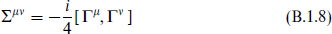
satisfy the SO(d − 1, 1) algebra

The generators Σ^2a,2a+1 commute and can be simultaneously diagonalized. In terms of the raising and lowering operators,

so ζ^(s) is a simultaneous eigenstate of the S_a with eigenvalues s_a. The half-integer values show that this is a spinor representation. The spinors form the 2^k+1-dimensional Dirac representation of the Lorentz algebra SO(2k + 1, 1).

The Dirac representation is reducible as a representation of the Lorentz algebra. Because Σ^µν is quadratic in the Γ matrices, the ζ^(s) with even and odd numbers of do not mix. Define

which has the properties

The eigenvalues of Γ are ±1. The conventional notation for Γ in d = 4 is Γ₅, but this is inconvenient in general d. Noting that

we see that Γ_ss′ is diagonal, taking the value +1 when the s_a include an even number of and −1 for an odd number of . The 2^k states with Γ eigenvalue (chirality) +1 form a Weyl representation of the Lorentz algebra, and the 2^k states with eigenvalue −1 form a second, inequivalent, Weyl representation. For d = 4, the Dirac representation is the familiar four-dimensional one, which separates into 2 two-dimensional Weyl representations,

Here we have used a common notation, labeling a representation by its dimension (in boldface). In d = 10 the representations are

For an odd dimension d = 2k + 3, simply add Γ^d = Γ or Γ^d = −Γ to the Γ matrices for d = 2k + 2. This is now an irreducible representation of the Lorentz algebra, because Σ^µd anticommutes with Γ. Thus there is a single spinor representation of SO(2k + 2, 1), which has dimension 2^k+1.

Majorana spinors

The above construction of the irreducible representation of the Γ matrices shows that in even dimensions d = 2k + 2 it is unique up to a change of basis. The matrices Γ^µ* and −Γ^µ* satisfy the same Clifford algebra as Γ^µ, and so must be related to Γ^µ by a similarity transformation. In the basis s, the matrix elements of Γ^a± are real, so it follows from the definition (B.1.2) that Γ³, Γ⁵, …, Γ^d−1 are imaginary and the remaining Γ^µ real. This is also consistent with the explicit expression (B.1.7). Defining

one finds by anticommutation that

For either B₁ or B₂ (and only for these two matrices),

It follows from eq. (B.1.18) that the spinors ζ and B⁻¹ζ* transform in the same way under the Lorentz group, so the Dirac representation is its own conjugate. Acting on the chirality matrix Γ, one finds

so that either form for B will change the eigenvalue of Γ when k is odd and not when it is even. For k even (d = 2 mod 4) each Weyl representation is its own conjugate. For k odd (d = 0 mod 4) each Weyl representation is conjugate to the other. Thus in d = 4 we can designate the representations as 2 and rather than 2 and 2′, but in d = 10, only as 16 and 16′

Just as the gravitational and gauge fields are real, various spinor fields satisfy a Majorana condition, which relates ζ* to ζ. This condition must be consistent with Lorentz transformations and so must have the form

with B satisfying (B.1.18). Taking the conjugate gives ζ = B*ζ* = B*Bζ, so such a condition is consistent if and only if B*B = 1. Using the reality and anticommutation properties of the Γ-matrices one finds

A Majorana condition using B1 is therefore possible only if k = 0 or 3 (mod 4), and using B2 only if k = 0 or 1 (mod 4). If k = 0 both conditions are possible but they are physically equivalent, being related by a similarity transformation.

A Majorana condition can be imposed on a Weyl spinor only if B*B = 1 and the Weyl representation is conjugate to itself. For k odd, which is d = 0 or 4 (mod 8), it is therefore not possible to impose both the Majorana and Weyl conditions on a spinor: one can impose one or the other. Precisely for k = 0 mod 4, which is d = 2 (mod 8), a spinor can simultaneously satisfy the Majorana and Weyl conditions. Majorana–Weyl spinors in d = 10 play a key role in the spacetime theory of the superstring, and Majorana–Weyl spinors in 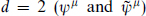play a key role on the world-sheet.

Extending to odd dimensions, Γ^d = ±Γ, and so the conjugation (B.1.19) of Γ^d is compatible with the conjugation (B.1.17) of the other Γ^µ only for B₁, so that k = 0 or 3 (mod 4). In all, a Majorana condition is possible if d = 0, 1, 2, 3, or 4 (mod 8). When the Majorana condition is allowed, there is a basis in which B is either 1 or Γ and so commutes with all the Σ^µν. In this basis the Σ^µν are imaginary.

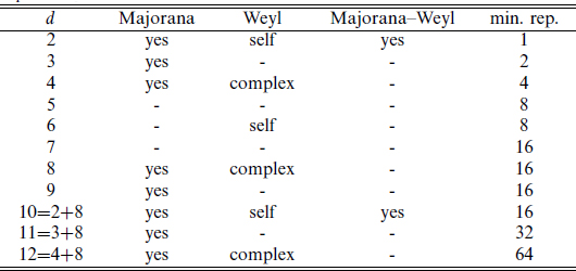
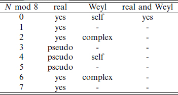
All these results are summarized in the table B.1. The number of real parameters in the smallest representation is indicated in each case. This is twice the dimension of the Dirac representation, reduced by a factor of 2 for a Weyl condition and 2 for a Majorana condition. The derivation implies that the properties are periodic in d with period 8, except the dimension of the representation which increases by a factor of 16.

Table B.1. Dimensions in which various conditions are allowed for SO(d − 1, 1) spinors. A dash indicates that the condition cannot be imposed. For the Weyl representation, it is indicated whether these are conjugate to themselves or to each other (complex). The final column lists the smallest representation in each dimension, counting the number of real components. Except for the final column the properties depend only on d mod 8.

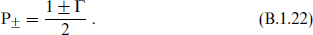
For d a multiple of 4, a spinor may have the Majorana or Weyl property but not both: conjugation changes one Weyl representation into the other. In fact, the two cases are physically identical, there being a one-to-one mapping between them. Define the chirality projection operators

Given a Majorana spinor ζ or a Weyl spinor χ, the maps

give a spinor of the other type, and these maps are inverse to one another.

The matrices −Γ^µT also satisfy the Clifford algebra. The charge conjugation matrix has the property

Using the hermiticity property

this implies that

Then for even d,

For odd d = 2k + 3, again only C = B₁Γ⁰ acts uniformly on Γ^µ for all µ; with this definition CΓ^µC⁻¹ = (−1)^k+1 Γ ^µT. In all cases,

Additional properties of the matrices B and C are developed in exercise B.1.

Product representations

We now wish to develop the decomposition of a product of spinor representations. A product of spinors ζ and χ will have integer spins and so can be decomposed into tensor representations. Recall the standard spinor invariant

Similarly

transforms as the indicated tensor. However, this involves conjugation of the spinor ζ. From the properties of C it follows that ζ^TC transforms in the same way as , so for the product of spinors without conjugation

transforms as a tensor.

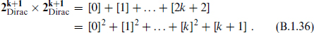
Starting now with the case of d = 2k + 3 odd, we claim that

for m ≤ k + 1 comprise a complete set of independent tensors. Here

is the completely antisymmetrized product. Without the antisymmetry these would not be independent, as the anticommutation relation would allow a pair of Γ matrices to be removed. The restriction m ≤ k + 1 comes about as follows. The definition of Γ implies in even dimensions that

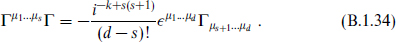
In odd dimensions, where Γ^d = ±Γ, it follows that the antisymmetrized products (B.1.33) for m and d − m are linearly related. There are no further restrictions, and the dimensions agree: 2^k+1 · 2^k+1 in the product of spinors and 2^2k+2 from the binomial expansion. Thus

where [m] denotes the antisymmetric m-tensor.

For even d = 2k + 2, the products of m and d — m Γ matrices are independent, and the same construction leads to

In the second line we have used the equivalence [m] = [d − m] from contraction with the -tensor. Again the dimensionality is correct.

To find the products of the separate Weyl representations, use

as follows from the definition of C. The tensor (B.1.32) is then nonvanishing if k + m is odd and the chiralities of ζ and χ are the same, or if k + m is even and the chiralities are opposite. This allows us to separate the product (B.1.36):

The relation (B.1.34) implies that the tensors of rank k + 1 = d/2 satisfy a self-duality condition with a sign that depends on the chirality of the spinor. A self-dual tensor representation can only be real for k even.

Some of the facts that we have deduced can also be verified quickly by considering the eigenvalues s_a. Consider the reality properties of the Weyl spinors. Conjugation flips the rotation eigenvalues s₁, …, s_k but not the boost eigenvalue s₀. For k even, this is an even number of flips and gives a state of the same chirality; for k odd it reverses the chirality. This is consistent with the third column of table B.1. For the tensor products of Weyl representations, note that the even-rank tensors [2n] (e.g. the invariant [0]) always contain a component with eigenvalues s_a = (0, 0, …, 0), while the odd-rank tensors do not. This would be obtained, for example, from the product of spinor components 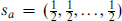and 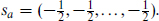For k even these have opposite chirality, as in the product (B.1.38c). For k odd they have the same chirality, as in the products (B.1.38a) and (B.1.38b).

Table B.2. Dimensions in which various conditions are allowed for SO(N) spinors.

Spinors of SO(N)

For SO(N) the analysis is quite parallel. For N = 2l, there is a 2^l-dimensional representation of the Γ-matrices which reduces to two 2^l−1-dimensional spinor representations of SO(2l), while for SO(2l + 1) there is a single representation of dimension 2^l. The reality properties can be analyzed as in the Minkowski case. Essentially one ignores µ = 0, 1, so SO(N) is analogous to SO(N + 1, 1), with the results shown in table B.2. Here real means the algebra can be written in terms of purely imaginary matrices. The term pseudoreal is often used for N = 3, 4, 5 mod 8, where the representation is conjugate to itself but cannot be written in terms of imaginary matrices.

The familiar case of a pseudoreal representation is the 2 of SO(3). This is conjugate to itself because it is the only two-dimensional representation, but it must act on a complex doublet. It should be noted, however, that two wrongs make a right — the product of two pseudoreal representations is real. Let the indices on u_ij both be SU(2) doublets, either of the same or different SU(2)s. Then the reality condition

is invariant. With just a single index, the analogous condition would force u to vanish. Incidentally, one can impose a Majorana condition on the 2 of SO(2, 1), consistent with table B.1. A real basis for the Γ-matrices is

Product representations are obtained as in the Minkowski case, with the result in N = 2l

For more than one timelike dimension, the analog of table B.1 or B.2 depends on the difference of the number of spacelike and timelike dimensions.

Decomposition under subgroups

We frequently consider subgroups such as

We can directly match representations by comparing the eigenvalues of S_a. In particular, for the case in which all the dimensions are even,

the Weyl spinors decompose

Another subgroup that has particular relevance for the superstring is

To describe this subgroup, consider again the complex linear combinations (B.1.2) of Γ-matrices, where a = 1, …, n. A general SO(2n) rotation will mix the Γ^a+ both among themselves and with the Γ^a−. The subgroup that mixes the Γ^a+ only among themselves is U(n) = SU(n) × U(1). Now let us consider how the spinor representation decomposes. Again we start with the spinor ζ annihilated by all the Γ^a−. This condition Γ^a−ζ = 0 is invariant under U(n) rotations so that ζ rotates at most by a phase. Thus

where the U(n) charge, indicated by the subscript, has been normalized to 2∑Sa. Acting with a raising operator adds an SU(n) index and increases the U(1) charge by 2, giving

where [k] refers to the k-times antisymmetrized n of SU(n). The completely antisymmetrized [n] is the same as [0] = 1, while 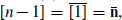and so on. Decomposing further into the Weyl representations, the last term [0]n is in the 2ⁿ⁻¹, and the successive terms alternate. Thus in particular for

we have

A relation that arises often is

To see this, combine the four components of a vector into a 2 × 2 matrix

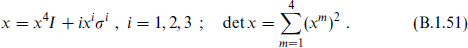
The length of x is invariant under independent left- and right-hand SU(2) rotations

giving the decomposition (B.1.50). Then

The decomposition of the vector is just eq. (B.1.52), while those of the spinors can be derived in various ways.

B.2 Introduction to supersymmetry: d = 4

The familiar conserved quantities, such as energy-momentum, angular momentum, and charge, transform as vectors, tensors, and scalars under the Lorentz group. It is also possible for a conserved quantity to transform as a spinor. Such a supersymmetry (SUSY) will relate the properties of fermions to those of bosons. Supersymmetry is a feature of all consistent string theories. Further, as discussed in section 16.2, there is good reason to expect that it will be found with particle accelerators.

In this appendix we summarize the various results that will be needed in the text. We are interested in the algebras, their representations, the transformations of the fields, and the invariant actions. The reader should be able to follow the derivation of the various representations (massless, standard massive, and BPS massive). However, the transformations and actions require detailed calculation, and so for these we simply cite for reference some of the key results.

d = 4, N = 1 supersymmetry

According to table B.1, the smallest spinor in four dimensions has four real degrees of freedom. As shown in eq. (B.1.23) this can be described either as a Weyl spinor, with two complex components, or as a Majorana spinor, with four components satisfying a reality condition.

The smallest d = 4 supersymmetry algebra would have one Weyl or Majorana spinor of supercharges. Again these are identical, the same four linearly independent supercharges described in two different notations; we will use the Majorana description. A more general supersymmetry algebra in d = 4 would have 4N supercharges. For N > 1 this is known as extended supersymmetry. In any number of dimensions the ratio of the number of supercharges to the smallest spinor representation is denoted by N. However, the structure of the theory depends more on the actual number of supercharges than on the ratio N, so subsequent sections are organized according to this total number. For pedagogic purposes we find it convenient in this section to start with the smallest algebra and build up, but later we will start with the largest algebra and work downwards, from 32 to 16 to 8. The number of supercharges need not be a power of 2, but in the great majority of examples it is and so these are the cases on which we focus.

The N = 1 supersymmetry algebra is uniquely determined to be

where Pµ is the spacetime momentum. The minus sign is due to our metric signature (− + … +). Recall that from the Majorana property,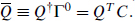

It is easy to work out the representations of this algebra. The massless and massive representations differ, and we consider the former first. For massless states choose a frame in which k₁ = k₀. The supersymmetry algebra becomes

In the s-basis, the Majorana condition becomes and the anticommutator becomes

The matrix elements of Q_−1/2,s1 must vanish in these momentum eigen-states because

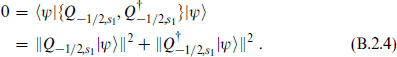
The remaining supercharges form a fermionic oscillator algebra. Defining

the supersymmetry algebra becomes

Starting from a state |λ such that

the algebra generates exactly one additional state

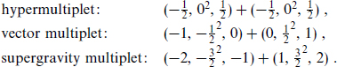
The massless irreducible multiplets thus each consist of two states with helicities differing by : one state in each multiplet is a fermion and one a boson. These are also representations of Poincaré symmetry. However, CPT, which appears to be an exact symmetry of string theory as it is of field theory, requires that each multiplet be accompanied by its conjugate with opposite helicities and quantum numbers. Thus we have the following multiplets:

The chiral multiplet consists of a multiplet and its CPT conjugate corresponding to a Weyl fermion and a complex scalar.

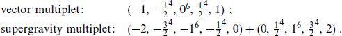
The vector multiplet plus contains a gauge boson and a Weyl fermion, both necessarily in the adjoint of the gauge group.

The gravitino multiplet plus contains an additional spin- gravitino and so is not relevant since there is only one supersymmetry and so only the gravitino in the graviton multiplet. This multiplet would be relevant if we had a larger supersymmetry and decomposed it into N = 1 representations.

The graviton multiplet plus contains the graviton and gravitino.

Massless particles with helicities greater than 2 are believed to be impossible to couple to gravity, and have not arisen in string theory.

In an N = 1 supersymmetric extension of the Standard Model, the Higgs boson and spin- fermions are in chiral multiplets. The Standard Model fermions cannot be in vector multiplets because the latter must be in the adjoint representation.

For massive representations, the anticommutator in the rest frame is

This is now two copies of the fermionic oscillator algebra,

Starting again from a state

the algebra generates the additional three states

For example, the massive chiral multiplet is the same as the CPT-extended massless multiplet. The multiplet is incomplete, even without CPT, because massive states must be a representation of the rotation group SU(2). Adding in we obtain a spin-1, two spin- and one spin-0 particle. These are the same states as a massless vector plus chiral multiplet, and can be obtained from them via the Higgs mechanism.

Actions with d = 4, N = 1 SUSY

From section 16.4 on, we need some results about d = 4, N = 1 supersymmetry transformations and invariant actions. We collect these here, without derivation. A general renormalizable theory will contain a number of massless chiral and vector multiplets; the larger massive multiplets can always be decomposed into these. The particle content of the massless chiral multiplet corresponds to a complex scalar field and a Majorana (or Weyl) spinor ψ. That of a massless vector multiplet corresponds to a gauge field Aµ and a Majorana (or Weyl) spinor λ. In each case it is useful, though not essential, to add a complex auxiliary field, a complex field F in the chiral multiplet and a real field D in the vector multiplet. We then have the following superfields

These have the supersymmetry transformations

and

in terms of a Majorana SUSY parameter ζ.

The most general renormalizable action is determined by the gauge couplings g_a (which of course must be equal within each simple group) and the superpotential W(Φ), which is a holomorphic function of the superfields. Also, for each U(1) gauge group there is an additional parameter ξ_a, the Fayet–Iliopoulos term. The Lagrangian density is

where

and

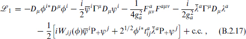
In are the kinetic terms, fermion masses and Yukawa couplings, while in are all terms involving the auxiliary fields. The are the gauge group representation matrices. Renormalizability requires the superpotential W to be at most cubic in the fields. Carrying out the Gaussian path integration over the auxiliary fields gives a scalar potential

where

The two terms in the potential are known respectively as the F-term, from the superpotential, and the D-term, from the gauge interaction.

An important nonrenormalization theorem states that the tree-level superpotential does not receive perturbative corrections. It is also important that this is only a perturbative statement, and that there can be nonperturbative corrections to the superpotential. An example of this arises in chapter 18.

Two kinds of internal symmetry are possible in supersymmetry. The first is a unitary rotation U_ij acting uniformly on all fields ⁱ, P+ψⁱ and Fⁱ in a given chiral multiplet. This is a symmetry if W is invariant. The gauge fields couple to such a symmetry. The second, known as an R symmetry, acts differently on different components:

Examining the action, for example the Yukawa terms, one sees that this is a symmetry provided the superpotential transforms as

In addition, the R symmetry must commute with the gauge symmetry.

Spontaneous supersymmetry breaking

As with an ordinary internal symmetry, spontaneous breaking of supersymmetry is signified by certain nonvanishing vacuum expectation values. In particular, consider

where Q_α is some component of the supercharge. We can assume the operator χ_β to be fermionic; otherwise, the expectation value vanishes automatically by Lorentz invariance. If supersymmetry is unbroken, Q_α|0 = 0|Q_α = 0 and all such vacuum expectation values vanish. Classically the condition for unbroken supersymmetry becomes

From the variations (B.2.14) and (B.2.15), it follows that a configuration is supersymmetric if the fields are position-independent, the gauge field is zero, and

Moreover, we see from the potential (B.2.19) that if such a configuration exists it will be a minimum of the energy. Supersymmetry will be spontaneously broken if there are no solutions to eqs. (B.2.25). The simplest example of a system with broken supersymmetry is a single superfield with superpotential

with ƒ a nonzero constant; then F = −ƒ* ≠ 0. This is rather trivial as it stands, but by coupling ₁ appropriately to other fields, for example

one obtains a theory with a nonsupersymmetric spectrum.

Higher corrections and supergravity

In the usual power counting in four dimensions, the scalar field and vector potential have dimension l⁻¹ and the spinors dimension l^−3/2, l being length. These are determined by the kinetic terms. It follows from the transformations (B.2.14) and (B.2.15) that the supersymmetry parameter ζ has dimension l^1/2, consistent with the product of two supersymmetry transformations being a translation. Also, the auxiliary fields Fⁱ and D^a have dimension l⁻². Including the l⁴ from d⁴x, the renormalizable action retains all terms that are relevant at long distance, that is, all terms of dimension lⁿ with n ≥ 0.

Power counting in renormalization theory is based on the scaling of the quantum fluctuations of the fields. However, in string theory we have encountered the phenomenon of moduli, scalar fields with flat potentials. These can have large classical values. In order to write an effective Lagrangian valid in all of moduli space,¹ we need a different power counting that assigns scalars scaling l⁰. Supersymmetry then assigns their fermionic partners scaling l^−1/2. We wish to keep all terms of the same order as the kinetic terms for these fields, and therefore all terms in the Lagrangian density having dimension l^m with m ≥ −2. In order to keep the kinetic terms for the gauge multiplet, assign A_µ scaling l⁰ and λ scaling l^−1/2. Finally, we assign the metric scaling l⁰, since it has a classical expectation value. Incidentally, this ‘moduli space’ power counting is the same in all dimensions, whereas the renormalization power counting is dimensiondependent.

In this approximation, the low energy effective action includes all the earlier terms plus additional ones. It depends now on three functions:

The superpotential W(Φ), which is still holomorphic but need no longer be cubic.

An arbitrary holomorphic function ƒ_ab(Φ) replacing the gauge coupling

The Kähler potential K(Φ, Φ^∗), which is a general function of the superfields.

Again there is a Fayet–Iliopoulos parameter ξ_a for each U(1). The full Lagrangian density is quite lengthy, so we give only the purely bosonic terms,

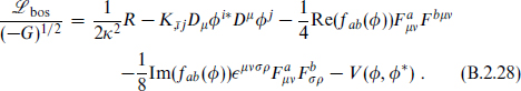
The potential is

Here K^j is the inverse matrix to and

The negative term proportional to κ² is a supergravity effect. The other terms generalize the earlier potential (B.2.19).

The kinetic term for the scalars is now field-dependent. The second derivative

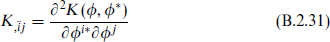
plays the role of a metric for the space of scalar fields, generalizing the flat metric δ_j of the renormalizable theory. The flat metric is the special case K = ⁱ*ⁱ. A metric of the form (B.2.31) is known as a Kähler metric. In a similar way, the function ƒ_ab() gives rise to a field-dependent (nonminimal) kinetic term for the gauge fields, as well as a field-dependent F₂ ∧ F₂ coupling. The metric (B.2.31) is invariant under Kähler transformations,

This is an invariance of the whole action provided also that the superpotential transforms as

This is important because in interesting examples the field space has a nontrivial topology and the Kähler potential is not globally defined.

The supersymmetry transformations of the fermions are

Here ψ_µ is the gravitino. The covariant derivative of the spinor ζ includes the spin connection. The variations (B.2.34) all vanish if the metric is flat, the gauge field zero, the scalars and ζ constant, and ∂_iW = D^a = W = 0.

Extended supersymmetry in d = 4

With several supersymmetries for A = 1, …, N, the straightforward generalization of the earlier algebra is

This is not the most general algebra, but we analyze it first. For massless particles, the earlier fermionic oscillator is replaced by N oscillators b_A. These generate 2^N states in a binomial distribution from helicity λ to helicity For example, for N = 2 the following massless multiplets are important:

In each case there are two SUSY multiplets, related by CPT. For states that are their own CPT conjugates, a half-hypermultiplet is allowed.

Let us note an important feature of these multiplets. If we just look at the SUSY multiplets, not making use of CPT, then all states in the multiplet have the same gauge quantum numbers because the supersymmetry charges commute with the gauge symmetries.² It follows that an N = 2 theory cannot have chiral gauge interactions. The only SUSY multiplets

with spin- states are the half-hypermultiplet and the vector multiplet. The former contains states of helicities with the same gauge quantum numbers and so is nonchiral. The latter is necessarily in the (real) adjoint representation and so is also nonchiral.

For N = 4 the multiplets are larger:

Finally, for N = 8 there is only a single possible representation:

Larger algebras would require helicities greater than 2, which is believed to be impossible (there are some uninteresting exceptions, such as free field theories). String theory has several times turned up loopholes in such statements, but not yet here.

Massive representations of extended supersymmetry similarly contain 2^2N states generated by b_1A and b_2A.

The most general extended supersymmetry algebra allowed by Lorentz invariance is

Here Z^AB is some set of conserved charges. It must be antisymmetric in AB due to the Majorana property and the antisymmetry of the charge conjugation matrix C.

To be precise, this is the most general algebra if we include only charges that can be carried by point particles. Including charges that can be carried by extended objects, additional terms appear. Rather than explain this here, we introduce it in its natural physical context: first in section 11.6, and then in more variety in chapter 13. The same caveat applies to the higher-dimensional algebras to be introduced later in this appendix.

To see the effect of the additional term consider a particle in its rest frame, for which the algebra becomes

Taking an eigenstate of the charges Z^AB, we can go to a basis in which

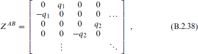
with q_i ≥ 0. The left-hand side of the algebra (B.2.37) is nonnegative as a matrix in (Aα, Bβ). The eigenvalues 2(m ± q_i) on the right-hand side must therefore also be nonnegative, implying the Bogomolnyi–Prasad–Sommerfield (BPS) bound

Thus the mass is bounded below by the charges, and in particular massless states must be neutral. If m is strictly greater than all the q_i, the massive representations are unaffected and contain 2^2N states. If the largest k qis are equal to one another and to m, the algebra requires 2k pairs of fermionic oscillators to annihilate the states, just as half the oscillators do for a massless representation. This gives a short or BPS representation with 2^2(N−k) states. If all the q_i are equal to one another and to m, the result is an ultrashort representation of dimension 2^N (for N even), the same as the massless representation.

B.3 Supersymmetry in d = 2

In this section we briefly make the connection with the world-sheet algebras of string theory. The smallest spinor representation in two dimensions is Majorana–Weyl and has one Hermitean component. The general algebra would have N Hermitean left-moving supercharges and Hermitean right-moving supercharges The algebra is

where now Z^AB need have no special symmetry. The superconformal generators G₀ and ₀ satisfy this algebra. Thus the R sector of the superconformal theory contains the supersymmetry algebra. In fact, this was one of several independent routes by which supersymmetry was first discovered.

The dimensional reduction of the d = 4, N = 1 supersymmetry algebra gives the d = 2 (2,2) algebra.

B.4 Differential forms and generalized gauge fields

Various antisymmetric tensor fields appear in supergravity and string theory. Differential forms are a convenient notation to minimize the bookkeeping of indices and combinatoric factors. A p-form A is simply a completely antisymmetric p-index tensor A_µ1…µp with the indices omitted. Because we encounter many different forms, we will denote the rank of any form by an italicized subscript, A_p. The product of a p-form A_p and a q-form B_q is written A_p ∧ B_q or simply A_pB_q, and is defined

Again, [ ] denotes antisymmetrization, averaging over permutations with a ±1 for odd permutations. The wedge product of a p-form A and q-form B has the property

The exterior derivative d takes a p-form into a (p + 1)-form:

It has the important property d² = 0.

The integral of a d-form is coordinate-invariant,

the transformation of the tensor offsetting that of the measure. Because of the antisymmetry, one must specify an orientation. Similarly, a p-form can be integrated over any p-dimensional submanifold. For a manifold with boundary one has Stokes’s theorem,

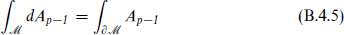
where is p-dimensional.

None of the above constructions requires a metric. In particular d contains only the ordinary derivative, but it is invariant due to the antisymmetry. One construction that does require a metric is the Poincaré dual, or, more properly, Hodge star. It is defined as

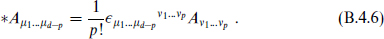
The Levi–Civita symbol _µ1…µd is defined to transform as a tensor. Thus with all lower indices its components are ±(−G)^1/2 and 0, while with all upper indices its components are ±(−G)^−1/2 and 0. One can check that on a p-form,

the +1 coming from the Minkowski signature.

One can also represent the above by introducing an algebra of d anticommuting differentials dx^µ, writing

The factorial just offsets the sum over permutations so that each independent component appears once. The product of a p-form A and a q-form B is then (B.4.1), and the exterior derivative is d = dx^ν∂_ν.

In this notation, an Abelian field strength, vector potential, and gauge transformation are written

In the non-Abelian case, writing the fields as matrices, these become

In the Abelian case there is a straightforward generalization to a p-form gauge transformation

The action is

A given component, say A_1…p+1, then appears with the canonical normalization for a real scalar, There is no straightforward non-Abelian generalization. For p = − 1, the gauge invariance is trivial and this describes a massless scalar.

Using the gauge invariance (B.4.11), we can set n^µA_µν1…νp = 0. The field equation then also implies k^µA_µν1…νp = 0 and k² = 0. The potential A_p+1 thus gives rise to a massless particle in the representation [p + 1] of the spin SO(d − 2).

Since [p + 1] = [d − p − 3] for SO(d − 2), a (p + 1)-form potential and a (d − p − 3)-form potential describe the same particle states. For d = 4 and p = 1, this is the familiar fact that B_µν describes the axion. We can also show this at the level of the fields. The Bianchi identity from F_p+2 = dA_p+1 and the equation of motion from the action (B.4.12) are

There is an obvious symmetry here: defining

simply switches the field equation and Bianchi identity, and in particular one can solve the new Bianchi identity in terms of a new potential where These theories are therefore equivalent, and one need consider only potentials of rank up to Again note that it is the field strength, not the potential, that is dualized. One can also see the equivalence in the action:

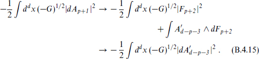
In the first action the potential A_p+1 is the variable of integration. In the second, F_p+2 is the variable of integration; the Bianchi identity is no longer automatic so a Lagrange multiplier has been introduced to enforce it. In the final form the original F_p+2 has been integrated out, leaving a gauge action for . In d = 4, this is electric–magnetic duality of Maxwell’s equations. In d = 3, it implies that a vector potential is equivalent to a massless scalar. In d = 2 a massless scalar is equivalent to a dual scalar; in fact, this is equivalent to the world-sheet T-duality X → X′. Again, note that it is the field strength to which the Poincaré duality is applied, not the potential.

For d = 2 mod 4, where ∗² = 1 on (d/2)-forms, it is consistent with the field equation and Bianchi identity to impose one of

These are consistent theories with half as many components. In d = 2 they correspond to the left- or right-moving parts of a massless scalar. The action (B.4.12) no longer gives the field equation, as

vanishes. There are more complicated actions which are not manifestly covariant.

B.5 Thirty-two supersymmetries

We now begin a survey of some of the supersymmetric theories that arise as low energy limits in string theory. A more complete treatment can be found in the references.

d = 11 supergravity

In four dimensions the largest supersymmetry algebra, N = 8, contains 32 supercharges. This same limit holds in higher dimensions, since we could reduce to four by compactifying on tori. Table B.1 then implies that d = 11 is the maximum in which supersymmetry can exist,³ since the spinor representations are too large for d ≥ 12. Although this exceeds by one the critical dimension of superstring theory, we will start with this case.

The Majorana spinor supercharge again satisfies the algebra

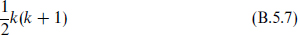
The massless irreducible representation contains 2⁸ = 256 states, half fermions and half bosons. By calculating the spins S₁, …, S₄ one finds that the graviton multiplet contains two bosonic representations of SO(9): a traceless symmetric tensor (the graviton) with components and a completely antisymmetric three-index tensor with 9 × 8 × 7/3! = 84 components for 128 in all. There is a single fermionic vector-spinor representation. The spinor index takes 16 values and the vector 9 values; 16 components vanish by a trace condition as in eq. (10.5.19), leaving 16 × 9 − 16 = 128 fermionic components.

With two or fewer derivatives there is a unique supersymmetric action, whose bosonic part is

with A₃ a 3-form potential and F₄ its 4-form field strength. The final Chern–Simons term is gauge-invariant in spite of the explicit appearance of A₃ because the term from the variation δA₃ = dλ2 vanishes by parts.

d = 10 IIA supergravity

By compactifying the d = 11 theory on a torus and keeping only the massless fields (dimensional reduction), we obtain a d = 10 theory with 32 supercharges. The d = 11 Majorana spinor becomes a d = 10 Majorana spinor, which reduces to one Majorana–Weyl spinor of each chirality,

The product of two spinors of the same chirality contains a vector, while the product of spinors of opposite chirality contains a scalar (eq. (B.1.38)), so from the eleven-dimensional algebra we deduce

Here Γ = Γ¹⁰ is from the toroidal dimension. A notable feature is the appearance of a central charge proportional to the Kaluza–Klein momentum. This is one of the ways that a central charge in the supersymmetry algebra can arise; additional central charges carried by extended objects are introduced in their physical context in section 13.2.

The dimensional reduction of the d = 11 theory leaves a scalar from G_{10 10}, a Kaluza–Klein vector from G_µ10, a 2-form potential from B_{µν 10} and a 3-form from B_µνσ. This is the same as the massless content of the IIA superstring, the scalar dilaton and the 2-form being from the NS–NS sector and the 1- and 3-forms from the R–R sector. This is no surprise because the large amount of supersymmetry determines the massless particle content completely. What is a surprise is that there really is an eleventh dimension hidden in the IIA string, invisible in perturbation theory but visible at strong coupling. This is discussed in chapter 14.

The action can be obtained by dimensional reduction; further details are given in section 12.1.

d = 10 IIB supergravity

There is another ten-dimensional supergravity, which is not obtained by compactifying an eleven-dimensional theory. This has two supercharges of the same chirality, which we can define to be 16. The algebra is

The graviton multiplet contains two scalars, the traceless symmetric graviton, two antisymmetric 2-forms, and a 4-form with self-dual field strength, for

bosonic states in all. This is the same as the massless content of the IIB superstring. More details are given in chapters 10 and 12.

d < 10 supergravity

The supergravities with 32 supercharges in d < 10 can be obtained by dimensional reduction of the IIA string, or equivalently of d = 11 supergravity. In this section we discuss some of the main features; this subject is relevant in particular to section 14.2. We need not consider the IIB string separately below d = 10, because after compactification on a circle it is T-dual to the IIA string (chapter 13).

Table B.3. Supergravities with 32 supercharges. The group G is a symmetry of the low energy supergravity theory, and the moduli space is locally G/H.

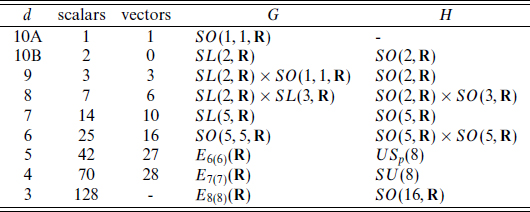
The first issue we wish to consider is the number of scalars. Compactifying k of the dimensions of d = 11 supergravity, there are

scalars from G_mn and

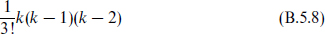
from B_mnp. Again m, n, p are compactified and µ,ν are noncompact. In addition, in d = 5, the Poincaré dual ∗(H_µνρσ) gives the field strength (gradient) for an extra scalar, as discussed at the end of section B.4. In d = 4, ∗(H_µνρm) gives 7 extra scalars. In d = 3, ∗(H_µνmn) gives extra scalars. Also in d = 3 the duals of the 8 Kaluza–Klein vectors give additional scalars. The total number is indicated in table B.3.

The second issue is the number of vectors: k from G_µn and from B_µmn. In addition there is one in d = 6 from ∗(H_µνρσ) and six in d = 5 from ∗(H_µνρm). In d = 4, ∗(H_µνmn) is just the magnetic description of the B_µmn vectors, and there are no vectors in d = 3 because we have converted them all to scalars by Poincaré duality. The results are summarized in the second column of the table. The gauge group is U(1)^n_V.

Third, there is no potential — the scalars are moduli — and the moduli space metric is completely determined by symmetry. The moduli spaces are cosets G/H, as listed in the table. The structure is the same as in the toroidal example in section 8.4, a coset of a noncompact group by a compact group. In the string case there was a further identification by the discrete T-duality group. This discrete identification does not affect the local structure of moduli space, and in particular not the effective action, and so it is not determined at this point by supersymmetry. Rather, it is determined by short-distance physics as is described in chapter 14. In the bosonic case the dilaton was decoupled, giving a separate space SO(1, 1, R) = R. Below d = 9 in table B.3 it combines with other moduli into a larger homogeneous space.

In each case, the noncompact group in the numerator is a global symmetry of the supergravity theory, and the compact group in the denominator is the unbroken symmetry at any point in moduli space. The notation E_n(n)(R) refers to an exceptional group with some sign changes in the algebra to make it noncompact, just as SO(n, m, R) is related to SO(n + m, R) and SL(n, R) to SU(n). The details of table B.3 are not at this point important, but it is interesting to see in chapter 14 how the structure fits into string theory.

For d = 4, the count in the table agrees with the N = 8 multiplet. To dimensionally reduce the supersymmetry algebra, separate the 11-dimensional 32-valued spinor index into a 4-valued SO(3, 1) index α and an 8-valued SO(7) index A. The 11-dimensional algebra (B.5.1) becomes

Here Γ^m factors into with being SO(7) Γ matrices. The factor of

must appear because Γ^m anticommutes with Γ^µ. Again, a central charge has arisen from the compact momenta. Since

the eigenvalues q_i of the central charge are all equal and any BPS multiplet will be ultrashort, with the same 256 states as a massless multiplet. In this case there is a simple explanation. The BPS condition is −P_µP^µ = P_mP^m, so a BPS multiplet is actually a massless multiplet from the higher-dimensional point of view.

The d = 4, N = 8 theory has 28 gauge bosons, but only the 7 Kaluza–Klein charges appear in the dimensionally reduced algebra (B.5.9). In fact, the full algebra contains all 28 gauge charges, the remainder arising from the extended-object charges in higher dimensions. The antisymmetric matrix Z^AB has precisely 28 components, so in general all are nonzero. The gauge charges can be organized into an antisymmetric matrix P^AB so that the algebra (after a chirality rotation to remove Γ₍₄₎) is

It should be noted that the compact momenta depend on the moduli, for example p = n/R for compactification on a single circle. When the central charge is written in terms of integer charges such as n, it has explicit dependence on the moduli.

B.6 Sixteen supersymmetries

d = 10, N = 1 (type I) supergravity

This algebra has a single Majorana–Weyl 16 supercharge. The massless vector representation has 16 states, 8_v + 8′ under the SO(8) little group. The supergravity multiplet is 8_v × (8v + 8′) as found in the bosonic and type I strings. The bosonic content is then a graviton, an antisymmetric tensor, and a dilaton from the supergravity multiplet plus dim g vectors from the gauge multiplets, g being the gauge group. The bosonic action is given in section 12.1. The action is classically invariant for any g, but as discussed in section 12.2 there are anomalies unless g = SO(32) or E₈×E₈.

d < 10 supergravity

Toroidal compactification of k dimensions gives supergravity with 16 supersymmetries in d = 10 − k. There are a total of k(k + r) + 1 moduli, r being the rank of the ten-dimensional gauge group g. The metric gives rise to moduli, the antisymmetric tensor to the Wilson lines to kr, and the original ten-dimensional dilaton to the final one. Of course g is SO(32) or E₈ × E₈, both having r = 16, in a consistent ten-dimensional theory, but here we are just using this as a trick to generate theories in lower dimensions. The reduced theories are parity-symmetric and have no anomalies, and so can have any g. In fact, various r < 16 theories can be obtained in string theory by slightly more complicated compactifications. The moduli space is as given explicitly by the Narain compactification of the heterotic string,

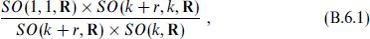
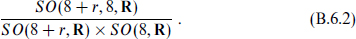
the SO(1, 1, R) being from the dilaton. In d = 4 the antisymmetric tensor gives another scalar, the axion, via Poincare duality; this combines with the dilaton to form SL(2, R)/SO(2, R). In d = 3 (k = 7), the Poincaré duals of the 14 + r vectors combine with the dilaton and the other moduli to enlarge the moduli space (B.6.1) to

Toroidal compactification gives gauge group U(1)^2k+r at generic points in moduli space, the original gauge group being broken to U(1)^r by Wilson lines. At special points it will be enhanced to various non-Abelian groups; the rank remains 2k + r.

d = 6, N = 2 supersymmetry

Under SO(9, 1) → SO(5,1) × SO(4), the ten-dimensional N = 1 supersymmetry decomposes

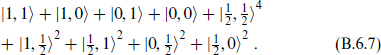
The (4, 2) has eight real components, forming a single complex 4. The 4 cannot have a Majorana condition imposed so the complex 4 is the smallest algebra in d = 6. The dimensionally reduced algebra is d = 6 (1, 1) supersymmetry, one supercharge in the 4 and one in the 4′. The only representation with spins ≤ 1 is the vector, which is the dimensional reduction of the d = 10 vector and so consists of one vector and four scalars.

Decomposing SO(5, 1) into the SO(1, 1) of the (0, 1)-plane and the transverse SO(4), the Weyl spinor supercharges decompose

These are complex representations, so their adjoints are independent operators. The representations of SO(1, 1) are all one-dimensional and are labeled by the helicity S₀. In the second equality of each line we have used the relation SO(4) = SU(2) × SU(2) and labeled the SU(2) representations by their spin j, so the notation is (s₀, j₁, j₂). As in section B.1, the generators annihilate the massless states. The latter then form a representation of the generators with these being Q_α and in the and of SU(2) × SU(2). Treating these as lowering operators and their adjoints as raising operators, by taking all combinations of raising operators one obtains the representations

Starting from an SU(2) × SU(2) multiplet annihilated by the lowering operators, the raising operators generate the representations

The supergravity multiplet is built on giving the states

The bosonic content, in the first line, is a graviton, an antisymmetric tensor, a scalar, and four vectors. The vector multiplet is built on |0, 0, giving

There is a second d = 6 algebra with 16 supercharges, the (2, 0) algebra with two complex 4 supercharges. The raising operators now form the representations

Acting on |0, 1, these produce the supergravity multiplet

whose bosonic content is a graviton and five anti-self-dual antisymmetric tensors. Acting on |0, 0 they produce the tensor multiplet

with self-dual antisymmetric tensor and five scalars.

d = 4, N = 4 gauge theory

The four-dimensional N = 4 algebra is

In this case only six of the gauge charges appear; in the heterotic string these are the ones coming from right-moving currents.

We now consider the effective renormalizable theory near a point of non-Abelian symmetry h. It will be useful to derive the full action and SUSY transformation by dimensional reduction of ten-dimensional supersymmetric Yang–Mills theory, whose Lagrangian density is

The gauge field and the gaugino λ (a Majorana–Weyl 16) are written in matrix notation, and M, N run from 0 to 9. The supersymmetry transformation is

Reducing M → µ, m, the Lagrangian density becomes

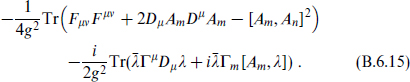
The six compact components of the gauge field become the six scalars A_m of the N = 4 vector multiplet. The 16 index separates into under SO(3, 1) × SO(6), so the ten-dimensional spinor becomes four Weyl spinors. Similarly the transformation laws reduce to

The potential

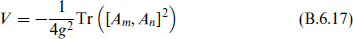
is nonnegative and vanishes only if [A_m, A_n] = 0 for all m, n. Thus, in the flat directions the A_m can be taken simultaneously diagonal, and the moduli are just the 6 rank(h) eigenvalues. At generic points the group is broken to U(1)^rank(h). We have seen this potential before, in eq. (8.7.11) for the D-brane moduli. This is no accident, as the T-duality that produces the D-brane has the effect of dimensionally reducing the open string Yang–Mills action.

Eq. (B.6.15) is the most general renormalizable action consistent with N = 4 global supersymmetry. It remains the most general action if we adopt the looser moduli space power counting described in section B.2, which would have allowed field-dependent kinetic terms. In other words, N = 4 global supersymmetry requires the moduli space to be flat. This is no contradiction with the curved moduli space (B.6.1) found in supergravity. The only scale there is the Planck scale, so the dimensionless variable is κA and the nonlinearities vanish in the limit κ → 0 where we ignore gravity.

The N = 4 Yang–Mills theory has a number of interesting properties, the first being that its beta function vanishes identically — the coupling does not run. Unlike most gauge theories, different values of g really give different theories, rather than being transmuted to a change of scale. It is easy to prove this statement, not just to all orders of perturbation theory but exactly. Consider for simplicity h = SU(2). Generically, A_m ∝ σ³ breaks SU(2) to U(1) at a scale

so the massless theory contains only an Abelian vector multiplet. Consider the gauge field kinetic term in the effective action. Its coefficient is −1/4g², but if the coupling runs in SU(2) we must figure out at what scale to evaluate g. The answer is v, because this is where SU(2) breaks and the coupling stops running. The scale v depends on the massless moduli, so what we really have is an effective Lagrangian density

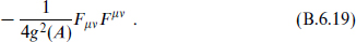
However, this is a field-dependent kinetic term, which we have just stated is inconsistent with N = 4 supersymmetry — unless in fact the coupling is independent of scale as claimed. This argument is typical of the recent analysis of supersymmetric gauge theories, but is particularly simple because of the large amount of supersymmetry.

B.7 Eight supersymmetries

d = 6, N = 1 supersymmetry

We start in six dimensions, the maximum in which a spinor with eight components is allowed according to table B.1. We obtain the massless representations as in eq. (B.6.6), where now

The supergravity multiplet, built on |, 1, is

containing the graviton, gravitino (which requires two copies of and the (0, 1) which is an anti-self-dual 2-form. The other relevant multiplets are built on and giving

The respective bosonic content is: two scalars; a vector; a self-dual tensor plus scalar.

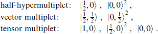
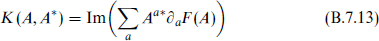
A general theory will have some number of vector, hyper-, and tensor multiplets. We describe the general bosonic Lagrangian, first in the most restrictive form of keeping only terms that would be renormalizable when reduced to four dimensions. The Lagrangian consists of gauge-invariant kinetic terms for the various fields and a potential for the hypermultiplets. The tensors must be neutral under the gauge group, so in this limit the tensor representation is decoupled from all other fields. To write the potential, we collect two half-hypermultiplets into a complex doublet of scalars with α the doublet index and i labeling the hypermultiplets.⁴ The N = 2 D-term is

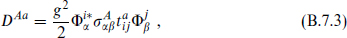
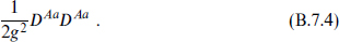
with the Pauli matrices (A = 1, 2, 3) and the group representation. The potential, determined entirely by the gauge symmetry, is

The interactions, incidentally, are nonrenormalizable in six dimensions.

Now consider the less restrictive moduli space action, where field-dependent kinetic terms are included, but with gravity still decoupled. Supersymmetry does not allow the gauge field kinetic term to depend on the hypermultiplet moduli, and it is allowed to depend on the scalar t in the tensor multiplets only in the precise form

The linear dependence is fixed because this term is related by supersymmetry to a coupling of the self-dual tensor,

where the tensor gauge invariance allows only the linear coupling. The term (B.7.6) is needed to cancel anomalies in a six-dimensional version of the Green–Schwarz mechanism, so these terms can arise only at exactly one loop, with a coefficient that is determined by the gauge quantum numbers of the hyper- and vector multiplets.

The hypermultiplet kinetic term may depend on the hypermultiplet moduli but not the tensor moduli. Representing the moduli by real fields ^r, one has

For the case of d = 4, N = 1 supersymmetry, we have explained in section B.2 that the moduli space must be Kähler, meaning that the 2n real moduli can be grouped into n complex fields ⁱ with the metric G_j = K_,j. Here the supersymmetry is doubled and the metric correspondingly more restricted: it must be hyper-Kähler. This means that there are three different complex Kähler structures, three different ways to group the real moduli into complex fields, each giving a Kähler metric. Further there is a relation between the three complex structures. Given any complex structure, a set of complex coordinates ⁱ and ⁱ*, we can define the tensor J by

This tensor can be defined for any complex manifold and is also known as the complex structure. We have defined it in a particular coordinate system but now can translate it to arbitrary coordinates. It satisfies J² = −1, a frame-independent statement. The three complex structures of the hyper-Kähler space are required to satisfy

These properties require the number of real moduli to be a multiple of 4.

An alternative characterization is as follows. There are 4m moduli, so a general metric (B.7.7) would have holonomy SO(4m). That is, parallel transport of a vector around a loop in moduli space brings it back to itself rotated by a general element of SO(4m). These ideas are familiar from general relativity, in the context of the spacetime manifold, but we emphasize that the manifold in question here is field space. Now consider the following SU(2) subgroup of SO(4m). We know that SO(4) = SU(2) × SU(2). Take the first SU(2) and replace the elements with m × m identity matrices to make a subgroup of SO(4m). The subgroup of SO(4m) that commutes with this SU(2) is Sp(m). Then a hyper-Kähler manifold is one for which the holonomy lies in this Sp(m) subgroup, the Js being the SU(2) generators.

d = 4, N = 2 supersymmetry

Let us first consider the reduction of the self-dual tensor multiplet from d = 6 to d = 5. The components B_µ5 become a vector. The dual ∗H_σρω would give the field strength of a second vector if the tensor were unconstrained, but due to the self-duality this is the same as H_µν5. Thus one has in all a vector and a scalar. This is the same as the content of the vector multiplet, where the scalar comes from the reduction of A₅, so these multiplets are identical in d = 5 and consequently in d = 4.

Thus in d = 4 we need consider only the hypermultiplet with four scalars, and the vector multiplet with two scalars A₄, A₅ from the six-dimensional vector. First in the renormalizable limit, the action includes the bosonic terms discussed in d = 6, the gauge-invariant kinetic terms and the potential (B.7.4). The potential has additional terms

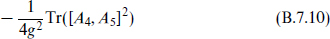
from reduction of the field strength and

where

The first term in M is from reduction of the covariant derivative; the parameters q_mij are allowed by supersymmetry and can be thought of as arising from a ‘dummy’ gauge field.

The potential has various flat directions. We discuss first the moduli space approximation with gravity still decoupled. Supersymmetry requires the kinetic term for the vector multiplet to depend only on the vector multiplet moduli and the kinetic term for the hypermultiplet to depend only on the hypermultiplet moduli. The latter is required to be a hyper-Kähler space just as in d = 6. The vector moduli space is also a Kähler metric with extra conditions. Namely, forming the complex scalars 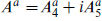with a indexing the gauge generators, the Kähler potential must be of the form

for some holomorphic prepotential F(A). The metric on moduli space is then

This is known as a rigid special Kähler metric.

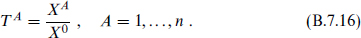
Turning on N = 2 supergravity, the moduli space acquires additional curvature as it did for N = 4, but it remains a direct product of hypermultiplet and vector multiplet moduli spaces. The hyper-Kähler metrics are replaced by quaternionic metrics, where the SU(2) holonomy is no longer zero but has a definite curvature of order κ². The vector moduli space becomes a special Kähler space. These spaces are also relevant to N = 1 compactifications of the heterotic string, so we describe them in some detail. For n hypermultiplets, it is useful to begin with n + 1 complex coordinates X^I with the projective identification

for any nonzero complex λ. One can also introduce invariant coordinates; for example, away from the subspace X⁰ = 0 the set

The low energy action is determined by a single complex function F(X), which must be homogeneous of degree 2 under the identification (B.7.15),

The Kähler potential is then

Under a projective transformation (B.7.15),

This is a Kähler transformation (B.2.32), so the metric is well defined on the projective space produced by the identification. The number of vectors is n + 1, including the one from the supergravity multiplet, so the fields for I = 0, …, n are independent. Their kinetic term is again determined by F and depends only on the vector multiplet moduli; its explicit form is left to the references.

The forms (B.7.15) and (B.7.18) are not invariant under arbitrary changes of coordinates: the coordinates X^I are known as special coordinates. The forms are clearly invariant under linear redefinitions of the special coordinates, but there is in fact a larger set of transformations that preserves the form, namely

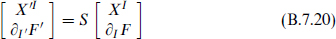
for S a 2(n + 1) × 2(n + 1) real symplectic matrix. As a final comment, in recent literature it has been noted that in special cases the symplectic transformation (B.7.20) gives a would-be gradient ∂_I′F′ whose curl is actually nonvanishing. For these the definition of special geometry needs to be generalized.

Exercises

B.1 In section B.1 we defined B and C in a particular basis. The properties (B.1.17) and (B.1.24) define them in general. Under a change of basis

for unitary U, find the transformations of B and C. Show that the properties (B.1.18), (B.1.19), (B.1.21), (B.1.25), and (B.1.27) are independent of such a change of basis. Determine the relations between B and B^T and between C and C^T, and show that these are independent of basis.

B.2 Extend the decomposition (B.1.44) to the general SO(d − 1, 1) → SO(d′ − 1, 1) × SO(d − d′), where some of the dimensions are odd.

B.3 Work out the details of the reduction of the d = 4, N = 1 supersymmetry algebra to the d = 2 (2, 2) algebra. Identify the central charges.

B.4 Verify eq. (B.4.7) for ∗² and derive the corresponding result for Euclidean space.

B.5 List the helicities (s₁, s₂, s₃, s₄) for the massless 8v + 8 open string states and show that these constitute a representation of the type I supersymmetry algebra.

¹ To be precise, the effective Lagrangian will still break down at particular points in moduli space, namely those points where extra massless fields occur. In the neighborhood of such a point, one needs an effective Lagrangian which includes these additional fields.

² There is an exception to this known as gauged supergravity, but it is not relevant to the gauge interactions of the Standard Model.

³ With two timelike dimensions a Majorana–Weyl spinor with 32 components is allowed at d = 12, but we will not try to figure out what this might mean.

⁴ If the scalars are in a pseudoreal representation of the gauge group, meaning that the conjugation matrix C_ij is antisymmetric, one can reduce to a half-hypermultiplet by the reality condition