18

Physics in four dimensions

We have now studied two kinds of four-dimensional string theory, based on orbifolds and on Calabi–Yau manifolds. We saw that the low energy physics of the weakly coupled heterotic string resembles a unified version of the Standard Model rather well. In this chapter we present general results, valid for any compactification. In most of this chapter we are concerned with weakly coupled heterotic string theories, but at various points we will discuss how the results are affected by the new understanding of strongly coupled strings.

18.1 Continuous and discrete symmetries

An important result holding in all string theories is that there are no continuous global symmetries; any continuous symmetries must be gauged. We start with the bosonic string. Associated with any symmetry will be a world-sheet charge

This is to be a symmetry of the physical spectrum and so it must be conformally invariant. Thus j_z transforms as a (1, 0) tensor and j as a (0, 1) tensor. We can then form the two vertex operators

These create massless vectors coupling to the left- and right-moving parts of the charge Q. Thus the left- and right-moving parts of Q each give rise to a spacetime gauge symmetry. If Q is carried only by fields moving in one direction, then only one of the currents and only one of the vertex operators is nonvanishing. Turning the construction around, any local symmetry in spacetime gives rise to a global symmetry on the world-sheet.

For type I or II strings the same argument holds immediately if we use superspace, writing

Superconformal invariance requires that J be a (, 0) tensor superfield and a (0, ) tensor superfield. Combined with ^µ or ψ^µ respectively, these give gauge boson vertex operators, so again this is a gauge symmetry in spacetime. The same is true for the heterotic string, using the bosonic argument on one side and the supersymmetric argument on the other.

The absence of continuous global symmetries has often been imposed as an aesthetic criterion by model builders in field theory, and we see that it is realized in string theory. There is a slight loophole in the argument, which we will discuss later in the section.

We have seen in the examples from earlier chapters that string theories generally have discrete symmetries at special points in moduli space. It is harder to generalize about whether these are local or global symmetries because the difference is subtle for a discrete symmetry: there is no associated gauge boson in the local case. The meaning of a discrete local symmetry was discussed in section 8.5 in the context of the field theory on the world-sheet. The simplest way to verify that a discrete symmetry is local is to find a point in moduli space where it is enlarged to a continuous gauge symmetry. For example, this is the case for the T-duality of the bosonic and heterotic strings. To see what this would mean, consider a spacetime with x⁸ and x⁹ periodic, with the radius R₈ a function of x⁹. Then R₈(x⁹) need not be strictly periodic; rather, it could also be that

This is the essence of a discrete gauge symmetry: that on nontrivial loops fields need be periodic only up to a gauge transformation. Since T-duality is embedded in the larger U-duality of the type II theory, the latter must be a gauge symmetry as well. Thus we could have a similar aperiodicity in the IIB string coupling, for example:

It is not clear that this is true of all discrete symmetries in string theory, but it seems quite likely.

P, C, T, and all that

We would like to discuss briefly the breaking of the discrete spacetime symmetries P, C, and T in string theory.

Parity symmetry P is invariance under reflection of any one coordinate, say X³ → –X³. It is not a good symmetry of the Standard Model, being violated by the gauge interactions. Classifying particles moving in the 1-direction by the helicity Σ²³ = s₁, the helicity + states form some gauge representation r₊, and the helicity – states some representation r-. Parity takes the helicity s₁ → –s₁, and so is a good symmetry only if r₊ = r_–. In the Standard Model it appears (barring the discovery of new massive states with the opposite gauge couplings) that r₊ ≠ r_–: the gauge couplings are chiral.

Let us consider the situation in string theory, starting with the ten-dimensional heterotic string. In ten dimensions states are labeled by their SO(8) representation. Parity again reverses the spinor representations 8 and 8′, and is a good symmetry only if the corresponding gauge representations are the same, r = r′. For the heterotic string, r is the adjoint representation while r′ is empty, so the gauge couplings are chiral and there is no parity symmetry. To see how this arises, note that the heterotic string action and world-sheet supercurrent (or BRST charge) are invariant if we combine the reflection X³ → −X³ with ψ³ → ‒ψ³. However, this also flips the sign of exp(πi) in the R sector, and so it is not a symmetry of the theory because the GSO projection restricts the spectrum to exp(πi) = +1.

Although the ten-dimensional spectrum is chiral, compactification to four dimensions can produce a nonchiral spectrum. This is true of toroidal compactification, for example, as one sees from the discussion in section 11.6. The point is that the theory is invariant under simultaneous reflection of one spacetime and one internal coordinate, say X³ and X⁹, as well as their partners ψ³ and ψ⁹. This is a symmetry of the action, supercurrent, and GSO projection, and so of the full theory. From the ten-dimensional point of view, it is a rotation by π in the (3,9) plane, but from the four-dimensional point of view it is a reflection of the 3-axis, combined with an internal action which gives negative intrinsic parity to the 9-oscillators. This symmetry reverses the momenta which are the charges under the corresponding Kaluza–Klein gauge symmetries, while leaving the other internal momenta invariant. Strictly speaking, it is therefore not a pure parity operation (which by the usual definition leaves gauge charges invariant) or a CP transformation (which inverts all charges), but something in between.

In the Z₃ orbifold example, the spectrum was found to be chiral. The orbifold twist removes all parity symmetries. Notice that simultaneous reflection of X^3,5,7,9, which takes Zⁱ ↔ Z, satisfies Pr = r²P and so commutes with the twist projection. However, to extend this action to the various spinor fields requires that P reflect ψ^3,5,7,9 and λ^2,4,6 as well. This acts on an odd number of the λ fermions and so does not commute with the current algebra GSO projection. The combined effect of the orbifold twist and the ψ and λ GSO projections removes all parity symmetry and leaves a chiral spectrum. Chiral gauge couplings arise in many other kinds of string compactification.

There is one interesting general remark. The chirality of the spectrum can be expressed in terms of a mathematical object known as an index. Separate exp(πi) into a spacetime part and an internal part, = ₄ + _K. For massless fermions moving in the 1-direction, 2s₁ = –i exp(πi₄), which in turn is equal to i exp(πi_K) due to the GSO projection. For massless R sector states the internal part is annihilated by G₀, so the net chirality (number of helicity + states minus helicity – states) in a given irreducible representation r is

the trace running over all states in the internal CFT which are in the representation r and are annihilated by G₀. One can now drop the last restriction on the trace,

The point is that any state |ψ with a positive eigenvalue ν under is always paired with a state G₀|ψ of opposite exp(πi_K), so these states make no net contribution to the trace. The state G₀|ψ cannot vanish because G₀G₀|ψ = ν| ψ.

Such a trace is known as an index: this can be defined whenever one has a Hermitean operator G₀ anticommuting with a unitary operator exp(πi_K). The index has the important property that it is invariant under continuous changes of the CFT. Under such a change, the eigenvalues ν of G²₀ change continuously, but the trace of exp(πi_K) at ν = 0 remains invariant because states can only move away from ν = 0 in pairs with opposite exp(πi_K). This invariance can also be understood from the spacetime point of view: a continuous change in the background fields can give mass to some previously massive states, but to make a massive representation one must combine states of opposite helicity.¹ Using this invariance, the index may often be calculated by deforming to a convenient limit. There is one subtlety that comes up in some examples: the index may change in certain limits due to states running off to infinity in field space.

Charge conjugation C leaves spacetime invariant but conjugates the gauge generators. In the Standard Model this is again broken by the gauge couplings of the fermions. For C invariance to hold, the fermion representations must satisfy r₊ = ₊ and r₋ = ₋. CPT invariance, to be discussed below, implies that r₊ = ₋ so that chiral gauge couplings violate C as well as P. Thus the orbifold example also violates C.

The combination CP takes r₊ → ₋ and so is automatically a symmetry of the gauge couplings as a consequence of CPT. In the Standard Model Lagrangian, CP is broken by phases in the fermion–Higgs Yukawa couplings. In the Z₃ orbifold example, the transformation that reverses X^3,5,7,9, ψ^3,5,7,9, and all of the λ^I for I odd is a symmetry of the action, the BRST charge, and all projections. From the point of view of the four-dimensional theory this is CP, because the action on the λ^I changes the sign of all the diagonal generators, which is charge conjugation. The Z₃ orbifold is thus CP-invariant. However, recall that there were many moduli. These included the flat metric background . The operation CP takes . Reality of the metric requires to be Hermitean, while CP requires it to be real. The generic Hermitean is not real, so CP is broken almost everywhere in moduli space. One must also consider other possible CP operations, such as adding discrete rotations of some of the Zⁱ, or permutations of the Zⁱ, to the transformation. These will be symmetries at special points in moduli space, but are again broken generically. This is also true for most other string compactifications: there will be CP-invariant vacua, but some of the many moduli will be CP-odd so that CP-invariance is spontaneously broken at generic points.

It is interesting to note that CP, like the discrete symmetries discussed earlier, is a gauge symmetry. The operation described above can be thought of as rotations by π in the (3,5) and (7,9) planes, combined with a gauge rotation. These are all part of the local symmetry of the ten-dimensional theory, though this is partly spontaneously broken by the compactification.

In local, Lorentz-invariant, quantum field theory the combination CPT is always an exact symmetry. It is easy to show that CPT is a symmetry of string perturbation theory, using essentially the same argument as is used to prove the CPT theorem in field theory. Consider the operation θ that reverses X^0,3 and ψ^0,3. If we continue to Euclidean time this is just a rotation by π in the (iX⁰,X³) plane and so is obviously a symmetry. The analytic continuation is well behaved because X^0,3 and ψ^0,3 are free fields. Clearly θ includes parity and time-reversal. To see that it also implies charge conjugation, recall that a vertex operator with k⁰ < 0 creates a string in the initial state, while a vertex operator with k⁰ > 0 destroys a string in the final state. If carries some charge q it creates a string of charge q. The operation θ does not act on the charges, so θ. also has charge q and so destroys a string of charge −q. Thus, θ takes a string in the in-state to the C-, P-, and T-reversed string in the out-state.

To make this slightly more formal, recall from section 9.1 that the S-matrix is given schematically by

where to be concise we have only indicated one vertex operator in each of the initial and final states. Then by acting with θ this becomes

The CPT operation is antiunitary,

so we see that CPT is θ combined with the conjugation of the vertex operator.

This argument is formulated in string perturbation theory. Elsewhere we have encountered results that hold to all orders of perturbation theory but are spoiled by nonperturbative effects. Without a nonperturbative formulation of string theory we cannot directly extend the CPT theorem, but we can ‘prove’ it by the strategy that we have used elsewhere: assert that the low energy physics of string theory is governed by quantum field theory, and then cite the CPT theorem from the latter. Still, there may be surprises; we can hope that when string theory is better understood it will make some distinctive non-field-theoretic prediction for observable physics.

The spin-statistics theorem is often discussed alongside the CPT theorem. The discussion in section 10.6 for free boson theories is easily generalized. Consider a basis of Hermitean (1,1) operators with definite Σ⁰¹ eigenvalue s₀ and βγ ghost number q. Now consider the OPE of such an operator with itself. In any unitary CFT, a simple positivity argument shows that the leading term in the OPE of a Hermitean operator with itself is the unit operator. Then

where the z- and -dependence follows from the weight of the exponential. For NS states, with integer spacetime spin, s₀ and q are integers, while for R states, with half-integer spacetime spin, they are half-integer. It follows that the operator product (18.1.11) is symmetric in the NS sector and antisymmetric in the R sector. The spacetime spin is thus correlated with world-sheet statistics, and the spacetime spin-statistics theorem then follows as in section 10.6. Again this is a rather narrow and technical way to establish this result.

The strong CP problem

In the Standard Model action CP violation can occur in two places, the fermion–Higgs Yukawa couplings and the theta terms

This is θ times the instanton number, the trace normalized to the n of SU(n). For the weak SU(2) and U(1) gauge interactions the fluctuations of the gauge field are small and the effect of S_θ is negligible, but for the strongly coupled SU(3) gauge field the nontrivial topological sectors make significant contributions. The result is CP violation proportional to θ in the strong interactions. The limits on the neutron electric dipole moment imply that

The CP-violating phases in the fermion–Higgs couplings are known from kaon physics not to be much less than unity. Understanding the small value of θ is the strong CP problem.

One proposed solution, Peccei–Quinn (PQ) symmetry, is automatically incorporated in string theory. In eq. (16.4.13) we found the coupling

Aside from this term, the action is invariant under

known as PQ symmetry. The field a, which would be massless if the symmetry (18.1.15) were exact, is the axion. The axion and the θ-parameter appear only in the combination , so θ has no physical effect: it can be absorbed in a redefinition of a. The effective physical value θ_eff is . The strong interaction produces a potential for a, which is minimized precisely at θ_eff = 0 because at this point the various contributions to the path integral add coherently. The weak interactions induce a nonzero value, but this is acceptably small.

The axion a is known as the model-independent axion because the coupling (18.1.14) is present in every four-dimensional string theory: the amplitude with one B_μν vertex operator and two gauge vertex operators does not depend on the compactification. Unfortunately, the model-independent axion may not solve the strong CP problem. There are likely to be several non-Abelian gauge groups below the string scale. Low energy string theories typically have hidden gauge groups larger than SU(3), and the corresponding strong interaction scales are Λ_hidden > Λ_QCD. We will see later in the chapter that this is a likely source of supersymmetry breaking.

The model-independent axion couples to all gauge fields. The gauge group with the largest scale Λ gives the largest contribution, so that the axion sets the θ-parameter for that gauge group approximately to zero. In a CP-violating theory, the θ-parameters for the different gauge groups will in general differ, so that θ_QCD remains large. Nonperturbative effects at the string scale may also contribute to the axion potential.

Another difficulty is cosmological. The axion a, being closely related to the graviton and dilaton, couples with gravitational strength κ. In other words, the axion decay constant is close to the Planck length. A decay constant this small leads to an energy density in the axion field today that is too large; it takes a rather nonstandard cosmology to evade this bound.

Both problems might be evaded if there were additional axions with appropriate decay constants. In Calabi–Yau compactifications there are shift symmetries (17.5.2) of the background, T^A → T^A + i^A. Further, the threshold corrections discussed in section 16.4 induce the coupling (18.1.14) to the gauge fields. However, these are only approximate PQ symmetries, because world-sheet instantons generate interactions proportional to

These spoil the PQ symmetries and generate masses for the axions b^A. There is some suppression if v^A/2πα′ is large, and possibly additional suppression from light fermion masses, which appear in relating the instanton amplitudes to the actual axion mass. However, the suppression must be very large, so that the axion mass from this source is well below the QCD scale, if this is to solve the strong CP problem.

In the type I and II theories the scalars from the R–R sector are also potential axions. As discussed in section 12.1, their amplitudes vanish at zero momentum, implying a symmetry C → C + for each such scalar. In addition they can have the necessary couplings to gauge fields. They receive mass from D-instanton effects.

In summary we have potentially three kinds of axion — model-independent, and R–R — which receive mass from three kinds of instanton — field theory, world-sheet, and Dirichlet. Not surprisingly, one can show that these are related by various string dualities. It may be that in some regions of parameter space the axions are light enough to solve the strong CP problem. There may also be additional approximate PQ symmetries from light fermions coupling to some of the strong groups. Or it may be that the solution to the strong CP problem lies in another direction, depending on details of the origin of CP violation.

Incidentally, these PQ symmetries are continuous global symmetries, seemingly violating the result obtained earlier. The loophole is that the world-sheet charge Q vanishes in each case — strings do not carry any of the PQ charges. We know this for the R–R charges; for the others it follows because the axion vertex operator at zero momentum is a total derivative. However, since in each case these are not really symmetries, being violated by the various instanton effects, the general conclusion about continuous global symmetries evidently still holds.

The arguments thus far are based on our understanding of perturbative string theory, but it is likely that the conclusion also holds at strong coupling. If a symmetry is exact at large g, it remains a symmetry as g is taken into the perturbative regime, since this is just a particular point in field space. At weak coupling it can then take one of two forms. It could be visible in string perturbation theory, meaning that it holds at each order of perturbation theory; it is then covered by the above discussion. Or, it could hold only in the full theory; the duality symmetries are of this type, but these are all discrete symmetries.

18.2 Gauge symmetries

Gauge and gravitational couplings

In sections 12.3 and 12.4 we obtained the relation between the gauge and gravitational couplings of the heterotic string in ten dimensions:

If we compactify, then by the usual dimensional reduction

with V the compactification volume. The relation between the parameters in the four-dimensional action is then the same,

Also, the actual physical values of the couplings depend on the dilaton as² e^Φ₄, but this enters in the same way on each side so that

This derivation is valid only in the field-theory limit, but with one generalization it holds for any four-dimensional string theory. For gauge bosons with polarizations and momenta in the four noncompact directions, the explicit calculation (12.4.13) of the three-gauge-boson amplitude involves only the four-dimensional and current algebra fields and so is independent of the rest of the theory. The only free parameter is the parameter from the current algebra, which appeared in the three-gauge-boson amplitude as ^−1/2. Thus the general result is

For completeness³ let us recall that is the coefficient of z⁻²δ^ab in the j^aj^b OPE, and that the gauge field Lagrangian density is defined to be

The parameter differs from the quantized level of the current algebra through the convention for the normalization of the gauge generators, which can be parameterized in terms of the length-squared of a long root, ψ² = 2/k. The common current algebra convention is ψ² = 2 so that = k. The common particle physics convention is that the inner product for SO(n) groups is the trace in the vector representation, and the inner product for SU(n) groups is twice the trace in the fundamental representation. Both of these give ψ² = 1 so that . We should emphasize that it is the quantized level k that matters physically — for example, it determines the allowed gauge representations — but that when we deal with expressions that require a normalization of the generators (like the gauge action) it is generally the parameter that appears.

It is interesting to consider the corresponding relation in open string theory. The ten-dimensional coupling was obtained in eq. (13.3.31),

Under compactification this becomes

Unlike the closed string relation, this depends on the compactification volume.

Gauge quantum numbers

For a gauge group based on a current algebra of level k, only certain representations can be carried by the massless states. The total left-moving weight h of the matter part of any vertex operator is unity. Since the energy-momentum tensor is additive,

the contribution of the current algebra to h is at most unity. This leaves two possibilities. Either the current algebra state is a primary field with h ≤ 1, or it is a descendant of the form

Let us consider the latter case first. The current j^a has h = 1, so for bosons the remainder of the matter vertex operator has weight (0, ). One possibility is ψ^μ, which just gives the gauge boson states. There could also be (0, ) fields from the internal CFT, but we will see later in the section that this is inconsistent with having any chiral gauge interactions. For fermions the remainder of the matter vertex operator would have weight (0, ). This combines with the βγ ghost vertex operator to give a (0, 1) current. This is a spacetime spinor, and so is the world-sheet current associated with a spacetime supersymmetry. Thus there are massless fermions of this type only if the theory is supersymmetric, in which case they are the gauginos.

For massless states based on current algebra primaries, the restriction (11.5.43) limits the representations that may appear. For SU(2) at k = 1 only the 1 and 2 are allowed, while for SU(3) at k = 1 only the 1, 3, and are allowed.

In the Standard Model, there are several notable patterns in the gauge quantum numbers of the quarks and leptons: replication of generations, chirality, quantization of the electric charge, and absence of large (‘exotic’) representations of SU(2) and SU(3). We have seen in the orbifold and Calabi–Yau examples that multiple generations arise frequently in four-dimensional string theories. This is an attractive feature of higher-dimensional theories in general. The generations arise from massless excitations that differ in the compact dimensions but have the same spacetime quantum numbers. Chirality was discussed in section 18.1, and quantization of electric charge will be discussed in section 18.4. Finally, the absence of exotics, the fact that only the 1 and 2 of SU(2) and the 1, 3, and of SU(3) are found, is ‘explained’ by string theory if we assume that these gauge symmetries arise from k = 1 current algebras. Also, the only scalar in the Standard Model is the SU(2) doublet Higgs scalar, and from tests of this model it is known that no more than O(1%) of the SU(2) × U(1) breaking can come from larger representations.

Unfortunately, this is not a firm prediction of string theory. While the simplest four-dimensional string theories have k = 1, there is still an enormous number of tree-level string vacua with higher level current algebras. Also, as discussed in section 16.3, k = 1 is impossible if a grand unified group remains below the string scale. For SU(5) only the representations 1, 5, , 10, and are allowed, for SO(10) only 1, 16, , and 10, and for E₆ only 1, 27, and . In each case this includes the representations carried by the quarks, leptons, and the Higgs scalar that breaks the electroweak symmetry, but not the representations needed to break the unified group to SU(3) × SU(2) × U(1). The latter are allowed for levels k ≥ 2. We will return to this point in the next section.

Right-moving gauge symmetries

Thus far we have considered gauge symmetries carried by the left-moving degrees of freedom of the heterotic string. For these the conformal in-variance leads to a current algebra. For gauge symmetries carried by the right-movers, the superconformal algebra plus gauge symmetry give rise to a superconformal current algebra (SCCA). The matter part of the gauge boson vertex operator in the −1 picture is

with a weight (0, ) superconformal tensor field. Then

is a (0, 1) field. It is nontrivial because

Also, is a conformal tensor, annihilated by for n > 0, though not a superconformal tensor. The thus form a right-moving current algebra.

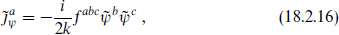
We take the current algebra to be based on a simple group g at level k, and for simplicity use the current algebra normalization (which is no problem, because we are about to see that these gauge symmetries will never appear in particle physics!). Using the Jacobi identity we can fill in the rest of the operator products,

In particular, the are free right-moving fields with a nonstandard normalization.

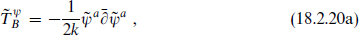
We can now carry out a generalization of the Sugawara construction. The product implies that if we define

where

then is nonsingular with respect to the . It follows that there are actually two current algebras. One is built out of the and has current and level k_ψ = h(g). The other commutes with the and has current and level k′ = k − k_ψ. We see that k ≥ h(g), with equality if and only if is trivial.

As in the Sugawara construction we can separate ,

where

and is nonsingular with respect to and . Further,

with

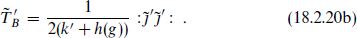
The remainders and are nonsingular with respect to both and . The CFT thus separates into three pieces, with central charges

The SCFT separates into only two pieces, because and are coupled in the supercurrent. In particular, the central charge for the SCFT is

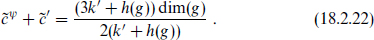
This lies in the range

The lower bound is reached only when vanishes, and the upper only for an Abelian algebra.

For an Abelian SCCA, the non-Abelian terms in the OPE (18.2.14) vanish. In particular, vanishes and k = k′, so a nontrivial theory requires that k′ ≠ 0. We can then normalize the currents to set k = k′ = 1. Writing the current as the derivative of a free boson, , gives

If there is a right-moving gauge symmetry below the string scale the gauge boson vertex operator must be periodic, and so the fermionic currents must always have the same periodicity as the supercurrent . This defines an untwisted SCCA.

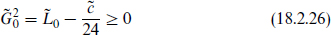
One can derive strong results restricting the relevance of right-moving gauge symmetries to physics. In the (1, 0) heterotic string,

1. If there are any massless fermions, then there are no non-Abelian SCCAs.

2. All massless fermions are neutral under any Abelian SCCA gauge symmetries.

3. If any fermions have chiral gauge couplings, then there are no SCCAs.

The first two results are sufficient to imply that the Standard Model SU(3) × SU(2) × U(1) gauge symmetries must come from the left-moving gauge symmetries in heterotic string theory. If, as it appears, the SU(3) × SU(2) × U(1) gauge couplings are chiral, then there are no right-moving gauge symmetries at all.

To show these, consider the vertex operator for any massless spin- state, whose matter part is

Here S_α is a spin field for the four noncompact dimensions, leaving a weight (1, ) operator from the internal theory. The Ramond generator is Hermitean, implying that

in any unitary SCFT. The internal theory here has central charge 9, and so the internal part of any massless spin- state saturates the inequality. Incidentally, this also implies that there can never be fermionic tachyons. Further, if the internal theory decomposes into a sum of SCFTs, , then the same argument requires that

within each SCFT.

Now suppose that one of these SCFTs is a non-Abelian SCCA. In the R sector the and are periodic. Then is bounded below by the zero-point energy dim(g) of the , and

This is strictly positive for all states, so massless fermions are impossible and the first result is established. For an Abelian SCCA, the same form holds with k′ = 1 and h(g) = 0, so equality is possible. However, the term j₀j₀ in makes an additional positive contribution unless the charge j₀ is zero for the state, establishing the second result.

The equivalence (18.2.24) means that a U(1) SCCA algebra has the same world-sheet action as a flat dimension. Further, as noted above, for an SCCA associated with a gauge interaction the periodicity of the fermionic current ψ is the same as that of the ψ^μ. Then if there is a U(1) SCCA the massless R sector ground states will be the same as those of a five-dimensional theory. The SO(4, 1) spinor representation 4 decomposes into one four-dimensional representation of each chirality, 2 + , so the massless states come in pairs of opposite chirality. In other words, the SO(4, 1) spin commutes with the GSO projection and (in the massless sector) with the superconformal generators, and so takes massless physical states into massless physical states of the opposite four-dimensional chirality. This establishes the third result, and shows that heterotic string vacua with right-moving gauge symmetries are not relevant to the Standard Model.

Gauge symmetries of type II strings

Now let us consider the possibility of getting the Standard Model from the type II string. Here, both sides are supersymmetric, so the vertex operators of gauge bosons are of one of the two forms

where ψ^a is associated with a left-moving SCCA and with a right-moving SCCA. For example, one could take the internal theory to consist of 18 right-moving and 18 left-moving fermions with trilinear supercurrents (16.1.29). This leads to gauge algebra g_R × g_L with g_R and g_L each of dimension 18. This can then be broken to the Standard Model by twists. This seems much more economical than the heterotic string, where the dimension of the gauge group can be much larger. However, we will see that the Standard Model does not quite fit into the type II string theory.

The same analysis as used in the heterotic string shows that only one of the two types of gauge boson (18.2.29) may exist. If there are chiral fermions in the R–NS sector there can be no left-moving SCCA, and if there are chiral fermions in the NS–R sector there can be no right-moving SCCA. In order to have both chiral fermions and gauge symmetries, the fermions must all come from one sector, say R–NS, and the gauge symmetries all from right-moving SCCAs.

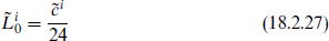
Now let us see that this does not leave room for the Standard Model. To be precise, it is impossible to have an SU(3) × SU(2) × U(1) gauge symmetry with massless SU(3) triplet and SU(2) doublet fermions. The internal part of any massless state has weight . This restricts the current algebra part to be either a primary state of the SCCA, annihilated by all the and for r, n > 0, or of the form . The latter is a gaugino, in the adjoint representation, so the triplets and doublets must be primary states instead. By the same argument as in the conformal case, the allowed representations for the primary states are restricted according to the level k′ of the current of the SCCA, so that k′ ≥ 1 in both the SU(2) and SU(3) factors in order to have doublets and triplets respectively. Noting that the central charge (18.2.22) increases with k′, the total central charge of the SCCAs is

This exceeds the total = 9 of the internal theory, so there is a contradiction.

This is an elegant argument, using only the world-sheet symmetries. However, progress in string duality has made its limitations clearer. Since all string theories are connected by dualities, we would expect that non-perturbatively a spectrum that can be obtained in one string theory can be obtained in any other. The most obvious limitation of the argument is that it applies only to vacua without D-branes, because the latter would have additional open string states. One might also wonder whether some or all of the Standard Model states can originate not as strings but as D-branes. As long as string perturbation theory is valid then all D-branes and other nonperturbative states should have masses that diverge as g → 0, so that string perturbation theory gives a complete account of the physics at any fixed energy. However, we will see in the next chapter that D-branes can become massless at some points in moduli space, and that this is associated with a breakdown of string perturbation theory.

18.3 Mass scales

There are a number of important mass scales in string theory:

1. The gravitational scale m_grav = κ⁻¹ = 2.4 × 10¹⁸ GeV, at which quantum gravitational effects become important; this is somewhat more useful than the Planck mass, which is a factor of (8π)^1/2 greater.

2. The electroweak scale m_ew, the scale of SU(2) × U(1) breaking, O(10²) GeV.

3. The string scale m_s = α′^−1/2, the mass scale of excited string states.

4. The compactification scale , the characteristic mass of states with momentum in the compact directions.

5. The grand unification scale m_GUT, at which the SU(3) × SU(2) × U(1) interactions are united in a simple group.

6. The superpartner scale m_sp, the mass scale of the superpartners of the Standard Model particles.

In this section we consider relations among these scales. Of course, there may be additional scales. The unification of the gauge group may take place in several steps, and there may be other intermediate scales at which new degrees of freedom appear. Also, these scales may not all be relevant. For example, when the internal CFT is a sigma model on a manifold large compared to the string scale, the idea of compactification applies. There are states with masses-squared of order , states which would be massless in the noncompact theory and which have internal momenta of order m_c. However, as m_c increases to m_s these states become indistinguishable from the various ‘stringy’ states, and compactification is not so meaningful. The internal CFT may have several equivalent descriptions as a quantum field theory, with ‘internal excitations’ and ‘stringy states’ interchanging roles. Similar remarks apply to the grand unification and supersymmetry scales.

For most of the discussion we will assume explicitly that the string theory is weakly coupled, and that the Standard Model gauge couplings remain perturbative up to the string scale. In this case it is possible to make some fairly strong statements. As we know from chapter 14, strong coupling opens up many new dynamical possibilities. The consequences for physics in four dimensions have not been fully explored; we will make a few comments at the end of the section.

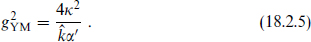
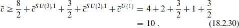
The relation between the string and gravitational scales follows from the relation (18.2.5) between the couplings,

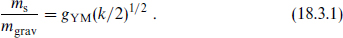
The quantities on the right are not too far from unity, so the string and gravitational scales are comparable. In the minimal supersymmetric model to be discussed below, the coupling g_YM at high energy is of order 0.7; for k = 1 this gives m_s ≈ 1.2 × 10¹⁸ GeV. This result is shown graphically in figure 18.1: plotted as a function of energy E are the four-dimensional gauge coupling 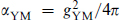and the corresponding dimensionless gravitational coupling κ²E². The scale where these meet is the expected scale of unification of the gravitational and gauge interactions, the string scale.

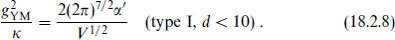
Now consider the compactification scale. Suppose that there are k dimensions compactified at some scale m_c m_s. Between the scales m_c and m_s, physics is described by a (4 + k)-dimensional field theory, in which a gauge coupling α_4+k has dimension m^−k and the gravitational coupling G_4+k has dimension m^−k−2. The behaviors of the dimensionless couplings α_4+kE^k and G_4+kE^k+2 are indicated in figure 18.1 by dashed lines. The gauge coupling rises rapidly from its four-dimensional value α_YM. Our assumption that the coupling remains weak up to the string scale then implies that the latter is not far above the compactification scale (in this section ‘scale’ always refers to energy, rather than the reciprocal length). Also, it presumably does not make sense for the compactification scale to be greater than the string scale, as illustrated by T-duality for toroidal compactification. Thus the string, gravitational, and compactification scales are reasonably close to one another. In open string theory, the quantitative relation (18.2.8) between the scales is different, but the reader can show that with the weak-coupling assumption these three scales are again close to one another.

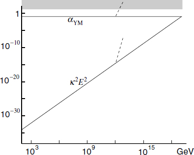
Fig. 18.1. The dimensionless gauge and gravitational couplings as a function of energy. On the scale of this graph we neglect the differences between gauge couplings and the running of these couplings. The dashed curves illustrate the effect of a compactification scale below the Planck scale, at 10¹² GeV in this example (the slopes correspond to all six compact dimensions being at this same scale, and are reduced if there are fewer). The shaded region indicates the breakdown of perturbation theory.

Next consider the unification scale. First let us review SU(5) unification of the Standard Model. The Standard Model gauge group SU(3)×SU(2)×U(1) can be embedded in the 5 representation of SU(5), with SU(3) being the upper 3×3 block, SU(2) the lower 2×2 block, and U(1) hypercharge the diagonal element

The SU(n) generators for the fundamental representation n are conventionally normalized . This is also true for U(1) if we define , in which case SU(5) symmetry implies

for the SU(3) × SU(2) × U(1) couplings. The hypercharge coupling g′ is defined by

The SU(5) prediction is then

The weak mixing angle θ_w is defined by . Before taking into account radiative corrections, the SU(5) prediction is sin² θ_w = . The same holds for standard SO(10) and E₆ unification, because SU(5) is just embedded in these.

For the purposes of the present section we will assume that the same relation (18.3.5) holds in string theory; in the next we will discuss the circumstances under which this is true. In both string theory and grand unified field theory, this tree-level relation receives substantial renormalization group corrections below the scale of SU(5) breaking. To one-loop order, the couplings depend on energy as

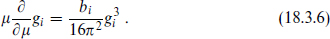
This integrates to

where . For a non-Abelian group the constant b_i is

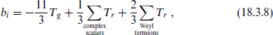
where and T_g = T_r=adjoint. For a U(1) group the result is the same with T_g = 0 and T_r replaced by q².

The couplings at the weak interaction scale M_Z are 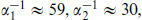and . Extrapolating the couplings α_i(μ) as in eq. (18.3.7), SU(5) unification makes the prediction (18.3.3) that at some scale m_GUT they become equal. This is often expressed as a prediction for sin²θ_w(m_Z): use and to solve for m_GUT and α_GUT, and then extrapolate downwards to obtain a prediction for . The prediction depends on the spectrum of the theory through the beta function (18.3.8).⁴ For the minimal SU(5) unification of the Standard Model,

For the minimal supersymmetric Standard Model, which consists of the Standard Model plus a second Higgs doublet plus the supersymmetric partners of these,

The experimental value is

The minimal nonsupersymmetric model is clearly ruled out. On the other hand, the agreement between the minimal supersymmetric SU(5) prediction and the actual value is striking, considering that a priori sin² θ_w(m_Z) could have been anywhere between 0 and 1. The agreement between the supersymmetric prediction and the actual value means that the three gauge couplings meet, with

In the nonsupersymmetric case, the disagreement with sin² θ_w(m_Z) implies that the three couplings do not meet at a single energy, but meet pairwise at three energies ranging from 10¹³ GeV to 10¹⁷ GeV.

To a first approximation, the unification scale (18.3.12) is fairly close to the string scale and so to the compactification and gravitational scales. This is also necessary for the stability of the proton. The running of the couplings is shown pictorially in figure 18.2. We should note that a direct comparison of the string and unification scales is not appropriate at the level of accuracy of the extrapolation (18.3.12). Rather, we should compare the measured couplings to a full one-loop string calculation: this is just the calculation (16.4.32). Ignoring for now the threshold correction, this relation is of the form (18.3.7) with the string unification scale (16.4.36)

We have inserted the relation (18.3.1) between the gauge and gravitational scales and then carried out the numerical evaluation using the unified coupling (18.3.12) and assuming k = 1. The resulting discrepancy between the string unification scale and the value in minimal SUSY unification is a factor of 30. This is larger than the experimental uncertainty, but small compared to the fifteen orders of magnitude difference between the electroweak scale and the string scale. This suggests that the unification and string scales are actually one and the same, so that not just the three gauge couplings but also the gravitational coupling meet at a single point; the apparent difference between the unification and string scales would then be due to some small additional correction.

Before discussing what such a correction might be, let us consider the consequences if the two scales actually are separated. This means that there is a range m_GUT < E < m_s in which physics is described by a grand unified field theory, with SU(3) × SU(2) × U(1) contained in SU(5) or another simple group. This theory is presumably four-dimensional, because even a factor of 30 difference between the string and compactification scales is difficult to accommodate. The unified group must then be broken to SU(3) × SU(2) × U(1) by the usual Higgs mechanism. As we have discussed in the previous section, this is not possible if the underlying current algebra is level one, because a Higgs scalar in the necessary representation cannot be lighter than the string scale. There do exist higher level string models in which such a separation of scales is possible.

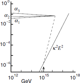
Fig. 18.2. The unification of the gauge couplings in the minimal supersymmetric unified model, and the near-miss of the gravitational coupling. The dashed line shows the potential effect of an extra dimension of the form S₁ /Z₂ at the scale indicated by the arrow.

An intermediate possibility is partial unification, embedding SU(3) × SU(2) × U(1) in one of

The group SU(5)′ × U(1) is known as flipped SU(5). Color SU(3) and weak SU(2) are embedded in SU(5) in the usual way, but hypercharge is a linear combination of a generator from SU(5) and the U(1) generator. String models based on flipped SU(5) have been studied in some detail. The group SU(4) × SU(2)_L × SU(2)_R is known as Pati–Salam unification. Color SU(3) is in the SU(4) factor, weak SU(2) is × SU(2)_L, and hypercharge is a linear combination of a generator from SU(4) and a generator from SU(2)_R. In the SU(3)³ group, sometimes called trinification, color is SU(3)_C, weak SU(2) is in SU(3)_L, and hypercharge is a linear combination of generators from SU(3)_L and SU(3)_R. When G is one of these partially unified groups and is embedded in a simple group as indicated in eq. (18.3.14), then the Standard Model group within G has the same embedding as in simple unification. The tree-level prediction for sin² θ_w(mZ) is therefore again , but the running of the couplings will of course be different between m_GUT and m_s. These partially unified groups can all be broken to the Standard Model by Higgs fields that are allowed at level one.

Now let us consider the corrections that might eliminate the difference between m_GUT and m_SU. The quoted uncertainties in the grand unified predictions come primarily from the uncertainty in the measured value of α3, and in the supersymmetric case from the unknown masses of the superpartners. There is a far greater uncertainty implicit in the assumption that the spectrum below the unification scale is minimal. Adding a few extra light fields, either at the electroweak scale or at an intermediate scale, can change the running by an amount sufficient to bring the unification scale up to the string scale.

There is also a threshold correction due to loops of string-mass fields. This is a function of the moduli, as in the orbifold example (16.4.38),

Although this correction reflects a sum over the infinite set of string states, its numerical value is rather small for values of the moduli of order 1. It can become large if the moduli become large. For example,

for large T_i, from the asymptotics of the eta function. For large enough T_i, in those models where the correction has the correct sign, this can account for the apparent difference between the string and unification scales.

Finally, in more complicated string models the tree-level predictions may be different and so also the predicted unification scale. We will discuss this somewhat in the next section.

All of these modifications have the drawback that a change large enough to raise the unification scale to the string scale will generically change the prediction for sin² θ_w by an amount greater than the experimental and theoretical uncertainty, so that the excellent agreement is partly accidental. Since the gauge couplings already meet, it would be simple and economical to leave them unchanged and instead change the energy dependence of the gravitational coupling so that it meets the other three. However, this seems impossible, since the ‘running’ of the gravitational coupling κ²E² is just dimensional analysis: the gravitational interaction is essentially classical below the string scale and quantum effects do not affect its energy dependence.

This is one point where the new dynamical ideas arising from strongly coupled string theory can make a difference. One way to change the dimensional analysis is to change the dimension! It does not help to have a low compactification scale of the ordinary sort: as shown in figure 18.1, all the couplings increase more rapidly but they do not meet any sooner. Consider, however, the strongly coupled E₈ × E₈ heterotic string compactified on a Calabi–Yau space K. From the discussion in chapter 14, this is the eleven-dimensional M-theory compactified on a product space

The scales of the two factors are independent; let us suppose that the space S₁/Z₂ is larger, so that its mass scale lies below the unification scale. The point is that the gauge and matter fields live on the boundary of this space, which remains four-dimensional, while the gravitational field lives in the five-dimensional bulk. The effect is as shown in figure 18.2: the gauge couplings evolve as in four dimensions, while the gravitational coupling has a kink. For an appropriate value of R₁₀, all four couplings meet at a point.

With the only data points being the low energy values of the gauge couplings, there is no way to distinguish between these various alternatives. If in fact supersymmetry is found at particle accelerators, then measurement of the superpartner masses will allow similar renormalization group extrapolations and may enable us to unravel the ‘fine structure’ at the string scale.

This brings us to the next scale, which is m_sp. The lower limits on the various charged and strongly interacting superpartners are of order 10² GeV. If supersymmetry is the solution to the hierarchy problem, the cancellation of the quantum corrections to the Higgs mass requires that the splitting between the Standard Model particles and their superpartners be not much larger than this,

Of all the new phenomena associated with string theory, supersymmetry is the one that is likely to be directly accessible to particle accelerators.

Finally, we should ask why the supersymmetry and electroweak scales lie so far below the others; we will discuss this briefly in section 18.8.

18.4 More on unification

In this section we collect a number of additional results on the relation between string theory and grand unification.

The first issue is the condition under which the grand unified relation g₁ = g₂ = g₃ holds in string theory at tree level. This is obviously the case in theories where a unified group remains unbroken below the string scale. It is also true if, as in the orbifold and Calabi–Yau cases, a unified group is broken at the string or compactification scale by twists. Although there is no scale at which the world looks like a four-dimensional grand unified theory, the inheritance principle guarantees that the equality of the tree-level couplings persists after the twist.

More generally one can make some statements just from current algebra arguments. The current algebra relation (18.2.5) between the gravitational coupling and any single gauge coupling implies that for the SU(2) and SU(3) gauge couplings

Thus the grand unified prediction α₂ = α₃ holds whenever the levels of the SU(3) and SU(2) current algebras are equal. In any case one expects that the levels are small integers, models with large levels having complicated spectra, so that if the levels are not equal their ratio differs substantially from unity. Since the unification scale can be determined from any pair of couplings, this implies a large change in the unification scale, spoiling the near-equality between the unification and string scales. Thus it is likely that, whatever the levels of the SU(2) and SU(3) current algebras, they are equal.

For the U(1) coupling there is no similar statement, because there is no level to give an absolute normalization to the current. One general result concerns the common situation that there is a continuous moduli space of vacua, all with an unbroken U(1) symmetry: if there are chiral fermions, then at tree level the coupling g₁, and so also sin²θ_w, is the same for all the connected vacua. To see this, write the U(1) current algebra in terms of a left-moving boson H(z). Let us consider how H might appear in the vertex operator for the modulus that interpolates between the vacua. The U(1) is assumed to be unbroken for all vacua, so the vertex operator must be invariant under H → H + — it can only contain derivatives of H. Dimensionally, the only operator that can then appear in a massless vertex operator is ∂H, and the whole matter vertex operator must be

for some (0, ) superconformal tensor . However, we know from section 18.2 that such tensors are inconsistent with chirality, so H cannot appear in the vertex operator at all. Expectation values of the U(1) current are then independent of the modulus, and therefore so is the gauge coupling.

A related issue is the quantization of electric charge. An isolated fractional multiple of the electron charge has never been seen in nature. The Standard Model has fractionally charged quarks, of course, but these are confined in hadrons of integer charge. It is therefore useful to work with

where the triality T, defined mod 3, is +1 for an SU(3) 3 and −1 for a . One can take T to be the SU(3) generator which is diag(1, 1,−2) in the 3 representation. Quarks are confined in states with T = 0 mod 3, so for all isolated states Q′ = Q_EM mod 1. The charge Q′ has been defined so as to be an integer for all Standard Model fields, so it follows that Q_EM is an integer for all isolated states.

Now consider this issue in string theory, starting with some special cases. If there is an SU(5) gauge group below the string scale, there can be no isolated fractional charges. In the SU(5) 5, the charge

is

Since Q′ is an integer for all states in the 5 and all representations can be obtained as tensor products of 5s, Q′ is an integer for all states and so Q_EM is an integer for all isolated states.

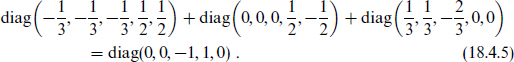
Now consider the case in which there is a level one SU(5) current algebra at the string scale, broken by twists to SU(3) × SU(2) × U(1). Let us represent this current algebra by free fermions λ^K± for K = 4, …, 8, with SU(3) acting on K = 4, 5, 6 and SU(2) acting on K = 7, 8 (the numbering is kept consistent with the orbifold and Calabi–Yau chapters). The current corresponding to Q′ is thus

In a sector with boundary conditions

the bosonized vertex operator

has charge

Thus there will be isolated fractional charges if there are twisted sectors with ν₆ ≠ ν₇. In fact there must be such sectors. Consider the gauge boson associated with the current λ⁶⁺λ⁷⁻. This carries the SU(3) × SU(2) representation (3,2) and is one of the SU(5) bosons that is removed by the twists that break the SU(5) symmetry. One of the twists must therefore have exp[2πi(ν₆ − ν₇)] ≠ 1, and the corresponding twisted sector has fractional Q′.

The lightest fractionally charged particle must be stable due to charge conservation. The number of fractional charges in ordinary matter is known to be less than 10⁻²⁰ per nucleon. If fractionally charged particles of mass m were in thermal equilibrium in the early universe at temperatures T > m, it is estimated that annihilation would only reduce their present abundance to approximately 10⁻⁹ per nucleon. Whether this is a problem depends critically on the masses of the fractionally charged states, whether all are near the string scale or whether some are near the weak scale. If all the fractional charges are superheavy then the situation is very similar to that with magnetic monopoles in grand unified theories. Diluting the density of relic monopoles was one of the original motivations for inflationary cosmology; this would also sufficiently dilute the fractional charges. It may also be the case that the universe was never hot enough to produce string-scale states thermally. Fractionally charged particles with masses near the weak scale are a potentially severe problem, unless they are charged under a new strongly coupled gauge symmetry and so confined.

In Calabi–Yau compactification the fractionally charged states are superheavy. The twist that breaks SU(5) is accompanied by a freely-acting spacetime symmetry, so that any string in the twisted sector of the gauge group will be stretched in spacetime. In orbifold compactifications there can be massless fractionally charged states from the twisted sectors, but the Calabi–Yau result suggests that superheavy masses are more generic.

Let us mention a generalization of the previous result. If the SU(3) and SU(2) gauge symmetries are at level one, and the tree-level value of sin²θ_w is the SU(5) value , and SU(5) is broken to SU(3) × SU(2) × U(1), then there are states of fractional Q′. To see this, write the SU(3) × SU(2) × U(1) current algebra in terms of free bosons, the diagonal currents being⁵

The current j_Y/2 is normalized so that the z⁻² term in the j_Y/2j_Y/2 operator product is times that of the non-Abelian currents, giving the tree-level value sin² θ_w = . Then

just as above, and Q′ = k⁷ − k⁶. If Q′ were an integer for all states, then the (1, 0) operator

would have single-valued OPEs with respect to all vertex operators. However, this would mean that the current algebra is larger than the assumed SU(3) × SU(2) × U(1); in fact, closure of the OPE gives a full SU(5) algebra and gauge group. So under the assumptions given there must be fractional charges. This is more general than the earlier result, the assumption of a twisted SU(5) current algebra having been replaced by a weaker assumption about the weak mixing angle.

There are various further generalizations. By an extension of the above argument it can be shown that if the current algebras are level one, and there are no states of fractional Q′, and SU(5) is broken, then the tree-level sin² θ_w must take one of the values . To make these values consistent with experiment takes a very nonstandard running of the couplings, suggesting that either the current algebras are higher level or that supermassive fractional charges should be expected to exist. One can also obtain constraints on higher level models, but they are less restrictive. We mention in passing that at higher levels we cannot use the same free-boson representation of the current algebras. Rather, simple currents, defined below eq. (15.3.19), play the role that exponentials of free fields play in the level one case.

If unconfined fractional charges do exist, electric charge is quantized in a unit e/n smaller than the electron charge. The Dirac quantization condition implies that any magnetic monopole must have a magnetic charge which is an integer multiple of 2πn/e. Various classical monopole solutions exist in string theories, and one expects that the minimum value allowed by the Dirac quantization is attained. Discovery of a monopole with charge 2π/e would imply the nonexistence of fractional charges, and so have implications for string theory through the above theorems.

The final issues are proton decay and neutrino masses. The details here are rather model-dependent, but we will outline some of the general issues. Two of the successes of the Standard Model are that it explains the stability of the proton and the lightness of the neutrinos. The most general renormalizable action with the fields and gauge symmetries of the Standard Model has no terms that violate baryon number B. This is termed an accidental symmetry, meaning that the long life of the proton is indirectly implied by the gauge symmetries. The allowed ΔB ≠ 0 terms of lowest dimension are some four-fermion interactions. These will be induced in grand unified theories by exchange of heavy gauge (X) bosons. The operators have dimension 6, so the amplitude goes as , and an estimate of the resulting proton lifetime is

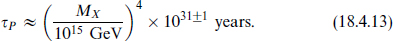
The experimental bound is of order 10³² years, so this is an interesting rate although very sensitive to the unification scale. Similarly, a mass for the Weyl neutrinos would violate lepton number, and L is another accidental symmetry of the Standard Model.

In supersymmetric theories there are gauge-invariant dimension 3, 4, and 5 operators that violate B and/or L. These are the superpotential terms

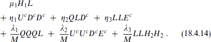
Here Q, U^c, D^c, L, and E^c are chiral superfields, containing respectively the left-handed quark doublet, anti-up quark, anti-down quark, lepton doublet, and the positron; H₁ and H₂ are chiral superfields containing the two Higgs scalars needed in the supersymmetric Standard Model. Gauge and generation indices are omitted. The dimension 3 term in the first line would generate a neutrino mass and so it must be that μ₁ ≤ 10⁻³ GeV, which is small compared to the weak scale and minuscule compared to the unification scale. The terms in the second line are of dimension 4, unsuppressed by heavy mass scales, and their dimensionless coefficients must be very small. For example, the first two terms together can induce proton decay, so η₁η₂ ≤ 10⁻²⁴. The terms in the third line are of dimension 5, suppressed by one power of mass; the proton decay limit λ_1,2 /M ≤ 10⁻²⁵ GeV⁻¹ requires a combination of heavy scales and small coefficients, while the lightness of the neutrino implies that λ₃ /M ≤ 10⁻¹³ GeV⁻¹. Thus any supersymmetric theory needs discrete symmetries to eliminate almost completely the dimension 3 and 4 terms and at least to suppress the dimension 5 terms unless they are not proportional to small Yukawa couplings. Several groups have argued that the necessary symmetries exist in various classes of string vacua. In many examples these seem to be associated with an additional U(1) gauge interaction broken in the TeV energy range.

There is at least one respect in which string theories, or at least higher-dimensional theories, may have an advantage over other supersymmetric unified theories. The SU(2) doublet Higgs scalar that breaks the weak interaction must have a mass of order the electroweak scale, while its color triplet GUT partners can mediate proton decay and so must have masses near the unification scale. It is possible to arrange the necessary mass matrix for these states without fine tuning, but the models in general seem rather contrived. String theory provides another solution. When an SU(5) current algebra symmetry is broken by twists, the low energy states do not in general fit into complete multiplets of the unified symmetry: some of the states are simply projected away. This is true somewhat more generally for any higher-dimensional gauge theory compactified to d = 4 with the gauge symmetry broken at the compactification scale by Wilson lines. In these cases one keeps certain attractive features, such as the unification of the gauge interactions and the prediction of mixing angle, but the undesired Higgs triplet need not be present.

18.5 Conditions for spacetime supersymmetry

Consider any four-dimensional string theory with N = 1 spacetime supersymmetry. We will show that there must be a right-moving N = 2 world-sheet superconformal symmetry, generalizing the results found in the orbifold and Calabi–Yau examples.

The current for spacetime supersymmetry is

We have separated the four-dimensional spin field into its 2 and components, denoted respectively by undotted and dotted indices. The four-dimensional spin fields have opposite values of , so the internal parts and parts must also have opposite values by the GSO projection. These are the vertex operators for the ground states of the compact CFT. They must each be of weight (0, ) in order that the total currents have weight (0, 1). As shown in section 18.2, this is the minimum weight for a field in this sector, and so parts annihilates both and .

The single-valuedness of the OPEs of and implies that

in order to cancel the branch cuts from the other factors. By unitarity, the coefficient of the unit operator in the OPE

cannot vanish, and so can be normalized to 1 as shown. The point of the following argument will be to show that the second term is also nonvanishing, so that there is an additional conserved current .

The OPE of supersymmetry currents is

As required by the supersymmetry algebra, the residue on the right-hand side is the spacetime momentum current; this is in the −1 picture just as in the ten-dimensional equation (12.4.18). It also follows from the supersymmetry algebra that the OPE of two undotted currents is nonsingular, implying that

The four-point function is then

where the OPEs as various points become coincident imply that f is a holomorphic function of its arguments. The ^−3/4 behavior as any of the (0, ) fields is taken to infinity then implies that f is bounded at infinity and so a constant. Taking the limit of the four-point function as ₁₂ → 0, the term of order implies that f = 1. The term of order then implies

so that in particular is nonzero. The further limits ₂₃ → 0, ₂₄ → 0, and ₃₄ → 0 then reveal that

As in the discussion of bosonization, the OPE implies that the expectation values of the current can be written in terms of those of a right-moving boson ,

The energy-momentum tensor separates into one piece constructed from the current and another commuting with it,

The OPE implies that

with ′ commuting with the current. The weight of the exponential is (0, ), the same as that of itself, so ′ is of weight (0, 0) and must be the identity. Thus the R ground state operators are functions only of the free field,

Now consider the supercurrent T_F of the compact CFT Since and are primary fields in the R sector and are annihilated by , we have

Using the explicit form (18.5.12), this implies

In other words,

Applying the Jacobi identity, one obtains the full (0, 2) superconformal OPE (11.1.4).

To summarize, the existence of N = 1 supersymmetry in spacetime implies the existence of N = 2 right-moving superconformal symmetry on the world-sheet. That is, there is at least (0,2) superconformal symmetry.

The various components of the spacetime supersymmetry current are now known explicitly in terms of free scalar fields; for example

Single-valuedness of this current with any vertex operator thus implies that all states have integer charge under

This integer charge condition is the generalization of the GSO projection.

The converse holds as well: if the (0, 1) world-sheet supersymmetry of the heterotic string is actually embedded in a (0, 2) or larger algebra, and if all states carry integer charge under the current , then the theory has spacetime supersymmetry. The argument is simple: if there is an N = 2 right-moving supersymmetry, then by bosonizing the current we can construct the operator (18.5.16). This is a (0, 1) field, a world-sheet current. By the integer charge assumption it is local with respect to all the vertex operators, and so has a well-defined action on the physical states. It is a spacetime spinor and so corresponds to a spacetime supersymmetry. Lorentz and CPT invariance generate the remaining components of the supersymmetry current (18.5.1). Combining these currents with ∂X^μ gives the gravitino vertex operators, so the supersymmetry is local.

The same argument can be applied to extended spacetime supersymmetry. The analysis is a bit longer and is left to the references, but we summarize the results. If there is N = 2 spacetime supersymmetry in the heterotic string, then the right-moving internal CFT separates into two pieces. The first, with = 3, is a specific (0, 2) superconformal theory: two free scalars and two free fermions forming the standard (0, 2) super-field discussed in section 11.1. The second, with = 6, must have (0, 4) supersymmetry but is otherwise arbitrary. If there is N = 4 spacetime supersymmetry, then the right-moving internal CFT consists precisely of six free scalars and six free fermions — in other words, it is a toroidal theory.

18.6 Low energy actions

In section 16.4 we obtained the low energy effective action for the Z₃ orbifold. Several important features of that action actually hold at string tree level for all four-dimensional string theories with N = 1 supersymmetry:

1. The Kähler potential is −κ⁻² ln(S + S*) plus terms independent of S.

2. The superpotential is independent of S.

3. The nonminimal gauge kinetic term is

Such general results are not surprising from a world-sheet point of view. The vertex operators for Φ₄ and a involve only the noncompact free fields X^μ and , which are independent of the compactification. The gauge boson vertex operators involve only these fields and the (1, 0) gauge currents, which again are universal up to the coefficient .

Rather than a detailed world-sheet derivation, it is very instructive to give a derivation based on the spacetime effective action. The introduction (16.4.12) of the axion field depends only on the four-dimensional fields and so is always valid. Under a shift a → a + the action changes only by a term proportional to

This is a topological invariant and vanishes in perturbation theory. In perturbation theory there is then a PQ symmetry

Second, there is a scale invariance: under

with the other bosonic fields invariant, the action changes by

This is just the statement that a constant dilaton only appears in the world-sheet action multiplying the world-sheet Euler number. The scaling (18.6.4) of the metric arises because the Einstein metric differs from the string metric by a function of the dilaton.

The PQ symmetry requires that the Kähler potential depend only on S + S*. In the kinetic term for S, the metric contributes a scaling t and so this term must be homogeneous in S; this determines the form given above for the Kähler potential.⁶ In the gauge kinetic term, the metric contributes no net t-dependence so f_ab must scale as t; by holomorphicity it must be proportional to S. The PQ symmetry then requires that it depend on no other fields, in order that the variation e multiply the topological term (18.6.2). The dependence on _a was obtained in section 18.2. It is often conventional to choose the additive normalization of the dilaton and the multiplicative normalization of the axion to eliminate g₄,

The physical value of the coupling is then

PQ invariance and the holomorphicity of the superpotential together require that the superpotential be independent of S. This is precisely consistent with the scaling of the action. To see this consider the term

in the potential (B.2.29). There is a scale-dependence t² from the metric and t⁻¹ from exp(κ²K), and so the action has the correct scaling if the superpotential is scale-invariant.

One of the great strengths of this kind of argument is that it gives information to all orders of perturbation theory, and even nonperturbatively. An L-loop term in the effective action will scale as

It follows from consideration of the potential again that an L-loop term in the superpotential scales as t^−L. PQ invariance requires (S + S*)^−L while holomorphicity requires S^−L, so only tree level is allowed, L = 0. This is an easy demonstration of one of the most important nonrenormalization theorems. The original proof in field theory involved detailed graphical manipulations; a parallel argument can be constructed in string perturbation theory using contour arguments. This nonrenormalization theorem has many important consequences. For example, particle masses or Yukawa couplings that vanish at tree level also vanish to all orders in perturbation theory (except in certain cases where D-terms are renormalized, as discussed in the next section).

For the gauge kinetic term f an L-loop contribution will scale as t^1−L. Again it must be holomorphic and PQ-invariant, allowing only L = 1, or L = 0 with the precise field dependence S. Thus, aside from this tree-level term f receives only one-loop corrections.⁷ With N = 1 supersymmetry there are no such constraints on the Kähler potential because it need not be holomorphic. An L-loop term (S + S*)^*L times any function of the other fields is allowed.

The PQ symmetry is broken by nonperturbative effects because the integral of F₂ Λ F₂ is nonzero for a topologically nontrivial instanton field. The superpotential and gauge kinetic terms can then receive corrections, which can often be determined exactly. We will see an example of a nonperturbative superpotential below.

One final point: there is a useful general result about the metric for the space of scalar fields. Suppose we have a compactification with some moduli ⁱ, which we take to be real. The world-sheet Lagrangian density ℒ_ws is a function of the ⁱ. One result of the analysis of string perturbation theory in chapter 9 was that the Zamolodchikov metric , which is the two-point function on the sphere, determines the normalization of the vertex operators. In other words, the inner product of the string states created by ⁱ and ^j is

This implies that the kinetic term for these fields is

Thus the Zamolodchikov metric is the metric on moduli space. This result does not depend on having world-sheet supersymmetry, although in this case we have the additional information that the manifold is complex and Kähler.

18.7 Supersymmetry breaking in perturbation theory

Supersymmetry breaking at tree level

Now we would like to consider the spontaneous breaking of supersymmetry, with particular attention to the fact that the supersymmetry breaking scale is far below the string scale. The first question is whether it is possible to find examples having this property at string tree level. In fact it seems to be essentially impossible to do so.

Here is an example which illustrates the main issue. Consider the heterotic string on a simple cubic torus, X^m ≅ X^m + 2πR_m for m = 4, …, 9, except that the translation in the 7-direction is accompanied by a π/2 rotation in the (8,9) plane. In other words, the (7,8,9)-directions form a cube with opposite faces identified, with a π/2 twist between one pair of opposite faces. This fits in the general category of orbifold models. However, the space is nonsingular because the combined rotation and translation has no fixed points. The rotation

is not in SU(3) and so all the supersymmetries are broken. However, there is a limit, R₇ → ∞, where the identification in the 7-direction becomes irrelevant and supersymmetry is restored. More explicitly, the effect of the twist is that p₇R₇ for any state is shifted from integer values by an amount proportional to the spin s₄, thus splitting the boson and fermion masses. This is the Scherk–Schwarz mechanism. The mass-squared splittings are of order and so go to zero as the 7-direction decompactifies. The obvious problem with this is that the supersymmetry breaking scale is tied to the compactification scale, which is inconsistent with the discussion in section 18.3. This linking of the supersymmetry breaking and compactification scales appears to be a generic problem with tree-level supersymmetry breaking. We could avoid it in the above example by taking instead the angle ₄ → 0; however, crystallographic considerations limit ₄ to a finite set of discrete values. Note that a twist acting on without acting on X^m would be a symmetry of the CFT for any values of ₄, but would not commute with and so would render the theory inconsistent.

There is a theorem that greatly restricts the possibilities for a large ratio of scales at tree level. The simplest way to obtain such a ratio would be to start with a supersymmetric vacuum and turn on a modulus that breaks the supersymmetry. Vacua in the neighborhood of the supersymmetric point would then have arbitrarily small breaking. However, this situation is not possible. If there is a continuous family of string vacua with vanishing cosmological constant, then either all members of the family are spacetime supersymmetric, or none is. We will give both a world-sheet and a spacetime demonstration of this.

On the world-sheet, we know that the supersymmetric point has (0,2) supersymmetry with a quantized U(1) charge. As we move away from this point either the supersymmetry must be broken to (0,1), which in particular implies that the U(1) in the (0,2) algebra is broken, or we must shift the quantization of the charge. To obtain either effect the vertex operator for the modulus must depend on the boson . It can be shown that this is impossible; the argument makes rather detailed use of the (0,2) world-sheet algebra so we defer it to the next chapter.

For the spacetime argument, let us denote the modulus as t, with t = 0 the supersymmetric point. The condition that the potential (B.2.29) be flat is

We assume that the modulus is neutral so that the D-term potential vanishes, but the argument can be extended to the case that it is not. Physically, the metric must be nonvanishing and nonsingular. As a differential equation for W, the condition (18.7.2) then implies that if W vanishes for any t then it vanishes for all t, as claimed. This shows that a continuous family of string vacua with zero cosmological constant cannot include both supersymmetric and nonsupersymmetric states in any theory with N = 1 supergravity, independent of string theory.

The Scherk–Schwarz mechanism gives arbitrarily small supersymmetry breaking, but the supersymmetric point R₇ = ∞ is at infinite distance. This evades the theorem but it is also what makes this example uninteresting. One could try to evade the theorem with a small discrete rather than continuous parameter. For example, the Sugawara SU(2) theories have c = 3 − 6/(k + 2) with k an integer, and so cluster arbitrarily closely to c = 3 as k → ∞. However, all attempts based on free, solvable, or smooth compactifications have run into the decompactification problem.

Supersymmetry breaking in the loop expansion

The conditions for unbroken supersymmetry are

Now let us suppose that these conditions are satisfied at tree level and ask whether loop corrections can lead to them being violated. We know that the superpotential does not receive loop corrections, so the first two conditions will continue to hold to all orders. For non-Abelian D-terms, the vanishing of the D^a is implied by the gauge symmetry, so the key issue is the U(1) D-terms.

The D-term potential is

Here δⁱ/δλ is the U(1) variation of the given scalar ⁱ. We have used what we know about the gauge kinetic term — the threshold correction f₁ is included for completeness, but it is subleading and makes no difference in the following discussion. The scaling property (18.6.9) (which includes the scaling of the (−G)^1/2 in the action) implies that an L-loop contribution to the potential scales as t^−L−1 and therefore as

Consider first the possibility of a nonzero Fayet–Iliopoulos term ξ being generated in perturbation theory. Expanding in powers of 1/S, the leading term in the potential is of order ξ²/Re(S). This is a tree-level effect, and so by assumption is absent.

Now consider the effect of gauging the PQ symmetry associated with S,

With the known form of the Kähler potential for S, the leading potential is

This is a two-loop effect, so D itself is a one-loop effect. To see the significance of the variation (18.7.6), consider the effect on the PQ coupling

This is not gauge-invariant but has just the right form to cancel against a one-loop anomaly in the gauge transformation, if the low energy fermion spectrum produces one. In fact, many compactifications do have anomalous spectra, and the anomaly is canceled by the variation (18.7.8) in a four-dimensional version of the Green–Schwarz mechanism. This is accompanied by cancellation of a gravitational anomaly. The induced D-term is proportional to Tr(Q), the total U(1) charge of all massless left-handed fermions.

Thus D ≠ 0 precisely if Tr(Q) ≠ 0, and then the supersymmetry of the original configuration is broken by a one-loop effect. The important question is whether the system can relax to a nearby supersymmetric configuration. The full D-term, including the other charged fields, is

and the potential is proportional to the square of this. If we can give the various ⁱ small expectation values, of order (S + S*)^−1/2, such that the D-term is set to zero while preserving W = ∂_iW = 0, then there is a supersymmetric minimum near the original configuration. In fact, in the known examples this is the case. Notice that while supersymmetry is restored, the new vacuum is qualitatively different from the original one. In particular, the U(1) gauge symmetry is now broken by the expectation value of e^S, and the gauge boson is massive. Being a one-loop effect, the gauge boson mass-squared is of order g²/8π² times the string scale. Thus the one-loop D-term produces a modest hierarchy of scales; this might be useful, for example, in accounting for the pattern of quark and lepton masses. Other massless particles may also become massive due to the shift in the ⁱ. These are effects that cannot occur with only F-terms in the potential.

It is also interesting to consider the case that the PQ-like symmetry associated with the (1,1) moduli T^A is gauged,

To leading order in S the potential is then

This is a tree-level effect. We are assuming that we have a supersymmetric tree-level solution, which is still possible on the submanifold of moduli space where q^A∂_AK = 0. The would-be moduli orthogonal to this submanifold are all massive. There is a natural origin for the gauge transformation (18.7.10). The imaginary part of T^A is the integral of B₂ over the 2-cycle N^A. In the heterotic string the gauge variation of B₂ is proportional to Tr(δλF₂), so if the U(1) field strength has an expectation value there is a transformation

This is automatically absent for Calabi–Yau compactification, because the integral of the flux measures the first Chern class. This is also another example of the difficulty of breaking supersymmetry by a small amount at tree level. It might seem that we could break the supersymmetry of the q^A∂_AK ≠ 0 vacua slightly by making F₂ small, but the integral of F₂ over any 2-cycle must satisfy a Dirac quantization condition. By a generalization of the monopole argument, q_i ∫ F₂ must be a multiple of 2π, where F₂ is proportional to any U(1) generator of E₈ × E₈, and q_i runs over the U(1) charges of all heterotic string states.

18.8 Supersymmetry beyond perturbation theory

An example

In the previous section, we saw that a vacuum that is supersymmetric at tree level usually remains supersymmetric to all orders of perturbation theory. Remarkably, it is known that in most tree-level N = 1 vacua the supersymmetry is broken spontaneously by nonperturbative effects. Our understanding of nonperturbative string theory is still limited, but below the string scale we can work in the effective quantum field theory. In fact, there is a reasonably coherent understanding of nonperturbative breaking of supersymmetry in field theory, and the low energy theories emerging from the string theory are typically of the type in which this breaking occurs. This subject is quite involved; there are several symmetry-breaking mechanisms (gaugino condensation, instantons, composite goldstinos), and a variety of techniques are needed to unravel the physics. Fortunately, we can get a good idea of the issues by focusing on the simplest mechanism, gluino condensation, in the simplest N = 1 vacua.

Consider any (2,2) compactification, with the visible E₆ possibly broken by Wilson lines. The hidden E₈ generally has a large negative beta function

The running coupling is

(for the present discussion we are not concerned about the small numerical difference between m_s and m_SU), and so becomes strong at a scale

This is below the string scale but above the scale where any of the visible sector groups become strong. Just as with quarks in QCD, the strong attraction causes the gauginos to condense,

Here and below ‘≈’ means up to numerical coefficients. As in QCD this condensate breaks a chiral symmetry, but in the pure supersymmetric gauge theory (gauge fields and gauginos only) it is known not to break supersymmetry.

In string theory at tree level the fields of the hidden E₈ couple to precisely one other light superfield, namely S. We have discussed the coupling of the dilaton and the axion to the field strength, but in addition supersymmetry requires a coupling between the auxiliary field and the gauginos

At scales below Λ₈ this looks like an effective interaction

From the general N = 1 action (B.2.16) this implies an effective superpotential⁸

This superpotential is nonperturbative, vanishing at large S faster than any power of 1/S. This is an example of the violation of a perturbative nonrenormalization theorem by nonperturbative effects. This superpotential is not PQ-invariant, which is consistent with the earlier discussion.

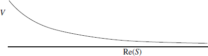
Fig. 18.3. The potential in a simple model of gluino condensation, as a function of the dilaton with other moduli held fixed.

What is more, this superpotential breaks supersymmetry. At tree level and to all orders of perturbation theory, the vacuum is supersymmetric for any value of S. Nonperturbatively,

is nonzero, which is the criterion (B.2.25) for the breaking of supersymmetry. This simple model is not satisfactory because the potential is roughly

The power of S + S* comes from the Kähler potential for S and from the two-loop beta function. At small coupling (large S), where the calculation is valid, the potential has the qualitative form shown in figure 18.3 and there is no stable vacuum. Rather, the system rolls down the potential toward the point Re(S) = ∞, where the theory is free and supersymmetric.

We will consider the problem of stabilizing the dilaton shortly, but for now let us see what happens if we assume that some higher correction, additional gauge group, or other modification gives rise to a stable supersymmetry-breaking vacuum at a point where S has roughly the value found in simple grand unified models. The number 100 seems large, but noting that |b₈| = 90 this is actually the typical scale for the S-dependence.

Having broken supersymmetry, the next question is how this affects the masses of the ordinary quarks, leptons, gauge bosons, and their superpartners. The only tree-level coupling of the supersymmetry breaking field S to these fields is again through a gauge kinetic term, that of the Standard Model gauge fields. Thus F_S has a coupling of the same form as (18.8.5) but to the ordinary gauginos. Inserting the expectation value for F_S gives a gaugino mass term,

The mass is

To solve the Higgs naturalness problem the masses of the Standard Model superpartners must be of order 10³ GeV or less. For the values S ≈ 100 and |b₈| = 90 of this simple model this is not the case, but because these parameters appear in the exponent a modest ratio of parameters S/|b| ≈ 12 would produce the observed large ratio of mass scales.

Once masses are generated for the Standard Model gauginos, loop corrections will give mass to the scalar partners of quarks and leptons. There is a simple reason why the (yet unseen) superpartners receive masses in this way while the quarks, leptons and gauge bosons do not: the latter masses are all forbidden by gauge invariance. Another feature to be understood is the negative mass-squared of the Higgs scalar, needed to break SU(2) × U(1), while the quark and lepton scalars must have positive masses-squared to avoid breaking baryon and lepton number. Again there is a simple general explanation, namely the one-loop correction to the Higgs potential coming from a top quark loop; the large top quark mass is just what is needed for this to work. The mass scale of the superpartners then determines the weak interaction scale.

The enormous ratio

thus arises ultimately from an exponent of order 10 in Λ₈, eq. (18.8.3). The renormalization group has this effect of amplifying modestly small couplings into large hierarchies. Thus, assuming the necessary stable vacuum, the enormous ratio of the weak and gravitational scales could emerge from a theory that has no free parameters.

We should point out that there is a distinction between the mass scale m_sp of the Standard Model superpartners and the scale of the supersymmetry-breaking expectation value. In fact,

or

This relation has a simple interpretation: the splittings in the Standard Model are given by the magnitude of the supersymmetry-breaking expectation value times the strength of the coupling between the Standard Model and the supersymmetry breaking. There has also been much consideration of field theory models in which the two sectors couple more strongly, through gauge interactions, and m_SUSY is correspondingly lower. Such models could arise in string theory, in (0,2) vacua.

The form of supersymmetry breaking in this particular model, from F_S, is known as dilaton-mediated supersymmetry breaking. Because the couplings of the dilaton are model-independent, the resulting pattern of superpartner masses is rather simple. In particular, the induced masses for the squarks and sleptons are to good accuracy the same for all three generations. This is important to account for the suppression of radiative corrections to rare decays (flavor changing neutral currents). More generally, radiative and other corrections can lead to a less universal pattern. Also, we have neglected all moduli other than the dilaton, but we will see below a simple model in which it is one of the Calabi–Yau moduli whose auxiliary field breaks supersymmetry.

The massless dilaton appears in the tree-level spectrum of every string theory, but not in nature: it would mediate a long-range scalar force of roughly gravitational strength. Measurements of the gravitational force at laboratory and greater scales restrict any force with a range greater than a few millimeters (corresponding to a mass of order 10⁻⁴ eV) to be several orders of magnitude weaker than gravity, ruling out a massless dilaton. We see from the present model that supersymmetry breaking can, and generically will, generate a potential for the dilaton. In this case there is no stable minimum, but the second derivative of the potential gives an indication of the typical mass

The superpotential (18.8.7) does not depend on any moduli other than S. This is because the scale Λ₈ is determined by the initial value of the gauge coupling, which at tree level depends only on S. We know that the one-loop correction to the gauge coupling depends on the other moduli, and this in turn induces a dependence in the superpotential. Thus if there is a stable minimum in the potential, generically all moduli will be massive.

Cosmological questions are outside our scope, but we note in passing that there is a potential cosmological problem with the moduli, in that their current energy density must not greatly exceed the critical density for closure of the universe. Typically the range of masses 10⁻⁷ GeV < m < 10⁴ GeV is problematic. Below this, the mass is sufficiently small not to present a problem; above it, the decay rate of the particles is sufficiently great. Masses at either end of the range give interesting possibilities for dark matter.

Let us give an optimistic summary. Start with the simplest heterotic string vacuum with N = 1 supersymmetry, namely a (2,2) orbifold or Calabi–Yau compactification. The result is a theory very much like the picture one obtains by starting from the Standard Model and trying to account for its patterns: gauge group E₆, chiral matter in the 27 representation, and a hidden sector that breaks supersymmetry (modulo the stabilization problem) and produces a realistic spectrum of superpartner masses. Of course, things may not work out so simply in detail; we know that the set of string vacua is vast, and we do not know any dynamical reason why these simple vacua should be preferred.

Another example

It is interesting to consider the following model,

The Kähler potential for T is based on the large-radius limit of Calabi–Yau compactification. Inclusion of a constant − w in the tree-level superpotential is consistent with the scaling and PQ transformations. After some cancellation, the potential is proportional to a square,

When W_;S = 0 the potential is minimized, and the value at the minimum is zero. Nevertheless supersymmetry is broken, as

This is intriguing: supersymmetry is broken nonperturbatively yet the vacuum energy is still zero. Also, the field T is undetermined, so there is a degenerate family of vacua with arbitrary supersymmetry-breaking scale W_;T. This is known as a no-scale model. The special properties of the potential depend on the detailed form of the Kähler potential and the superpotential, in particular the factor of 3 in the former and the fact that the latter is independent of T. Higher order effects will spoil this. For example, as we have noted above, threshold corrections will introduce a T-dependence into the superpotential.

Discussion

Since S ∝ g⁻², the superpotential (18.8.7) is of order exp[−O(1/g²)], which is characteristic of nonperturbative effects in field theory. It is not invariant under the PQ symmetry S → S + i but transforms in a simple way. This can be related to the breaking of PQ invariance by instantons, but the argument is rather indirect and we will not pursue it.

It is interesting to consider at this point the order exp[−O(1/g)] stringy nonperturbative corrections deduced from the large order behavior of string perturbation theory. For the type II string we were able to relate these to D-instantons, but there is no analogous amplitude in the heterotic string. In the type II theory the D-instanton gives rise to an effect that does not occur in any order of perturbation theory, the nonconservation of the integrated R–R 1-form field strength. In the heterotic string it is unlikely that the stringy nonperturbative effects violate the perturbative nonrenormalization theorems. They would give rise to effects proportional to one of the forms

with C a constant. The first form is holomorphic and the second is PQ-invariant. Corrections to the superpotential would have to be of the first form, but these have a complicated PQ transformation which is probably not allowed. In particular, it is believed that a discrete subgroup of the PQ symmetry is unbroken by anomalies; this would forbid the form exp(CS^1/2). The nonperturbative effects could then only modify the Kähler potential, but this in any case receives corrections at all orders of perturbation theory.

Now we return to the stabilization of the dilaton. One possibility is that there are two competing strong gauge groups. In this case the dilaton potential can have a minimum, which for appropriate choices of the groups can be at the weak coupling S ≈ 100 which is suggested by grand unification and needed for a large hierarchy. Another possibility is that a weak-coupling minimum can be produced by including the stringy nonperturbative corrections to the Kähler potential. It may seem odd that these corrections can be important at weak coupling, but it has been suggested that for the modestly small but not infinitesimal couplings of interest, the stringy nonperturbative effects can dominate the perturbative corrections. There may also be minima at very strong coupling, where the dual M-theory picture is more useful, or at couplings of order 1 which are close to neither limit.

Another idea would be that the potential really is as in figure 18.3 and that the dilaton is time-dependent, rolling toward large S. However, a brief calculation shows that these solutions cannot describe our universe: given the age of the universe, the supersymmetry breaking and gauge couplings would be far too small.

However, it is impossible to separate the stabilization of the dilaton from the cosmological constant problem. A generic potential on field space will have some number of local minima, but there is no reason that the value of the potential at any of the minima should vanish, either exactly or to the enormous accuracy required by the upper limit on the cosmological constant. So while the dilaton is stabilized, the metric is still ‘unstable,’ expanding exponentially, and the vacuum is not acceptable. The cosmological constant problem afflicts any theory of gravity, not just string theory. However, since predictive power in string theory is completely dependent on understanding the dynamics of the vacuum, any detailed discussion of the determination of the vacuum is likely to be premature until we understand why the cosmological constant is so small.

In any event, our current understanding would suggest that string theory has many stable vacua. Supersymmetry guarantees that the various moduli spaces with N = 2 and greater supersymmetry are exact solutions. In addition there are likely moduli spaces with N = 1 supersymmetry but no strong gauge groups and no breaking of supersymmetry. In addition there may be a number of isolated minima of approximate N = 1 supersymmetry, which are the ones we seek. There are also some string states of negative energy density. These are known to exist from one-loop calculations in nonsupersymmetric vacua with vanishing tree-level cosmological constant. The reader might worry that any vacuum with zero energy density will then be unstable. However, gravitational effects can completely forbid tunneling from a state of zero energy density to a state of negative energy density if the barrier between the two is sufficiently high. The conditions for this to occur are met rather generally in supersymmetric theories.

If there are many stable vacua, which of these the universe finds itself in would be a cosmological question, depending on the initial conditions, and the answer might be probabilistic rather than deterministic. This does not imply a lack of predictive power. Assuming that we eventually understand the dynamics well enough to determine the minima, there will likely be very few with such general features of the Standard Model as three generations. The key point is that because supersymmetry breaking leaves only isolated minima, there are no effective free parameters: the moduli are all determined by the dynamics.

This rather prosaic extrapolation is likely to be modified by new dynamical ideas. In particular, whatever principle is responsible for the suppression of the cosmological constant may radically change the rules of the game.

Exercises

18.1 Calculate the tree-level string amplitude with a model-independent axion and two gauge bosons.

18.2 Show from the explicit form of the string amplitudes that no scalar other than the model-independent axion has a tree-level coupling to F₂ Λ F₂.

18.3 Derive the conditions cited at the end of section 18.6 for a heterotic string theory to have N = 2 and N = 4 spacetime supersymmetry.

18.4 Calculate the Zamolodchikov metric for two untwisted moduli of the Z₃ orbifold and compare with the result obtained in chapter 16 by dimensional reduction.

18.5 Work out the one-loop vacuum amplitude for the twisted theory described at the beginning of section 18.7.

18.6 For the SO(32) heterotic string on the Z₃ orbifold, show that the gauge and mixed gauge–gravitational anomalies are nonzero. Show that they can be canceled by giving the superfield S the gauge transformation (18.7.6). Show that the resulting potential has supersymmetric minima.

18.7 If we integrate out the auxiliary field F_S, the couplings (18.8.5) lead to a tree-level interaction of four gauge fermions. Find this interaction using string perturbation theory. Note that it is independent of the compactification.

¹ This is one of those statements that, surprisingly, need no longer hold at strong coupling. We will discuss this further in sections 19.7 and 19.8.

² When Φ4 ≠ 0, the rescaling (16.4.6) changes the background value of the metric. To study the physics in a given background, as we are doing in this chapter, one should instead rescale

and the coefficient of the gravitational action is then the physical coupling κ = exp(Φ₄)κ₄.

³ We feel compelled to be precise about the factors of 2, but most readers will want to skip such digressions as this paragraph.

⁴ The experiment and theory are sufficiently precise that one must take into account the two-loop beta function, threshold effects at the weak and unified scales, and other radiative corrections to the weak interaction.

⁵ Only four free bosons are needed to represent the current algebra — the linear combination H⁴ + H⁵ + H⁶ + H⁷ + H⁸ does not appear. The notation is chosen to correspond to the bosonization of the earlier free Fermi representation.

⁶ Scale invariance seems to allow an additional term (C + C*) ln(S + S*), where C is any other superfield. To rule this out we appeal to the world-sheet argument that an off-diagonal metric is impossible because the CFT factorizes.

⁷ Such statements are often rather subtle in that one must be precise about what is not being renormalized. The discussion in section 16.4 of the physical coupling versus the Wilsonian action illustrates some of the issues.

⁸ This must be holomorphic in S, whereas the scale Λ₈ depends on Re(S). The point is that the phase of the condensate depends on the axion in just such a way as to account for the difference.