Chapter 5
Program Design and Analysis
Chapter Points
• Some useful components for embedded software.
• Models of programs, such as data flow and control flow graphs.
• An introduction to compilation methods.
• Analyzing and optimizing programs for performance, size, and power consumption.
5.1 Introduction
In this chapter we study in detail the process of creating programs for embedded processors. The creation of embedded programs is at the heart of embedded system design. If you are reading this book, you almost certainly have an understanding of programming, but designing and implementing embedded programs is different and more challenging than writing typical workstation or PC programs. Embedded code must not only provide rich functionality, it must also often run at a required rate to meet system deadlines, fit into the allowed amount of memory, and meet power consumption requirements. Designing code that simultaneously meets multiple design constraints is a considerable challenge, but luckily there are techniques and tools that we can use to help us through the design process. Making sure that the program works is also a challenge, but once again methods and tools come to our aid.
Throughout the discussion we concentrate on high-level programming languages, specifically C. High-level languages were once shunned as too inefficient for embedded microcontrollers, but better compilers, more compiler-friendly architectures, and faster processors and memory have made high-level language programs common. Some sections of a program may still need to be written in assembly language if the compiler doesn’t give sufficiently good results, but even when coding in assembly language it is often helpful to think about the program’s functionality in high-level form. Many of the analysis and optimization techniques that we study in this chapter are equally applicable to programs written in assembly language.
The next section talks about some software components that are commonly used in embedded software. Section 5.3 introduces the control/data flow graph as a model for high-level language programs (which can also be applied to programs written originally in assembly language). Section 5.4 reviews the assembly and linking process while Section 5.5 introduces some compilation techniques. Section 5.6 introduces methods for analyzing the performance of programs. We talk about optimization techniques specific to embedded computing in the next three sections: performance in Section 5.7, energy consumption in Section 5.8, and size in Section 5.9. In Section 5.10, we discuss techniques for ensuring that the programs you write are correct. We close with two design examples: a software modem as a design example in Section 5.11 and a digital still camera in Section 5.12.
5.2 Components for Embedded Programs
In this section, we consider code for three structures or components that are commonly used in embedded software: the state machine, the circular buffer, and the queue. State machines are well suited to reactive systems such as user interfaces; circular buffers and queues are useful in digital signal processing.
5.2.1 State Machines
State machine style
When inputs appear intermittently rather than as periodic samples, it is often convenient to think of the system as reacting to those inputs. The reaction of most systems can be characterized in terms of the input received and the current state of the system. This leads naturally to a finite-state machine style of describing the reactive system’s behavior. Moreover, if the behavior is specified in that way, it is natural to write the program implementing that behavior in a state machine style. The state machine style of programming is also an efficient implementation of such computations. Finite-state machines are usually first encountered in the context of hardware design.
Programming Example 5.1 shows how to write a finite-state machine in a high-level programming language.
Programming Example 5.1 A State Machine in C
The behavior we want to implement is a simple seat belt controller [Chi94]. The controller’s job is to turn on a buzzer if a person sits in a seat and does not fasten the seat belt within a fixed amount of time. This system has three inputs and one output. The inputs are a sensor for the seat to know when a person has sat down, a seat belt sensor that tells when the belt is fastened, and a timer that goes off when the required time interval has elapsed. The output is the buzzer. Appearing below is a state diagram that describes the seat belt controller’s behavior.
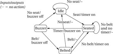
The idle state is in force when there is no person in the seat. When the person sits down, the machine goes into the seated state and turns on the timer. If the timer goes off before the seat belt is fastened, the machine goes into the buzzer state. If the seat belt goes on first, it enters the belted state. When the person leaves the seat, the machine goes back to idle.
To write this behavior in C, we will assume that we have loaded the current values of all three inputs (seat, belt, timer) into variables and will similarly hold the outputs in variables temporarily (timer_on, buzzer_on). We will use a variable named state to hold the current state of the machine and a switch statement to determine what action to take in each state. Here is the code:
#define IDLE 0
#define SEATED 1
#define BELTED 2
#define BUZZER 3
switch(state) { /* check the current state */
case IDLE:
if (seat){ state = SEATED; timer_on = TRUE; }
/* default case is self-loop */
break;
case SEATED:
if (belt) state = BELTED; /* won’t hear the buzzer */
else if (timer) state = BUZZER; /* didn’t put on belt in time */
/* default case is self-loop */
break;
case BELTED:
if (!seat) state = IDLE; /* person left */
else if (!belt) state = SEATED; /* person still in seat */
break;
case BUZZER:
if (belt) state = BELTED; /* belt is on---turn off buzzer */
else if (!seat) state = IDLE; /* no one in seat--turn off buzzer */
break;
}
This code takes advantage of the fact that the state will remain the same unless explicitly changed; this makes self-loops back to the same state easy to implement. This state machine may be executed forever in a while(TRUE) loop or periodically called by some other code. In either case, the code must be executed regularly so that it can check on the current value of the inputs and, if necessary, go into a new state.
5.2.2 Circular Buffers and Stream-Oriented Programming
Data stream style
The data stream style makes sense for data that comes in regularly and must be processed on the fly. The FIR filter of Application Example 2.1 is a classic example of stream-oriented processing. For each sample, the filter must emit one output that depends on the values of the last n inputs. In a typical workstation application, we would process the samples over a given interval by reading them all in from a file and then computing the results all at once in a batch process. In an embedded system we must not only emit outputs in real time, but we must also do so using a minimum amount of memory.
Circular buffer
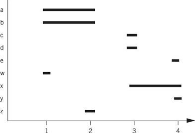
The circular buffer is a data structure that lets us handle streaming data in an efficient way. Figure 5.1 illustrates how a circular buffer stores a subset of the data stream. At each point in time, the algorithm needs a subset of the data stream that forms a window into the stream. The window slides with time as we throw out old values no longer needed and add new values. Because the size of the window does not change, we can use a fixed-size buffer to hold the current data. To avoid constantly copying data within the buffer, we will move the head of the buffer in time. The buffer points to the location at which the next sample will be placed; every time we add a sample, we automatically overwrite the oldest sample, which is the one that needs to be thrown out. When the pointer gets to the end of the buffer, it wraps around to the top.
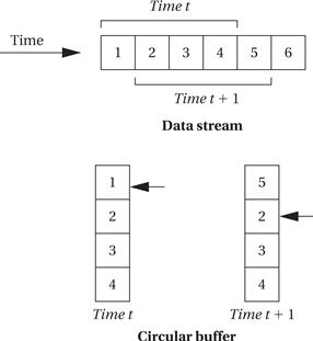
Figure 5.1 A circular buffer.
Instruction set support
Many DSPs provide addressing modes to support circular buffers. For example, the C55x [Tex04] provides five circular buffer start address registers (their names start with BSA). These registers allow circular buffers to be placed without alignment constraints.
In the absence of specialized instructions, we can write our own C code for a circular buffer. This code also helps us understand the operation of the buffer. Programming Example 5.2 provides an efficient implementation of a circular buffer.
High-level language implementation
Programming Example 5.2 A Circular Buffer in C
Once we build a circular buffer, we can use it in a variety of ways. We will use an array as the buffer:
#define CMAX 6 /* filter order */
int circ[CMAX]; /* circular buffer */
int pos; /* position of current sample */
The variable pos holds the position of the current sample. As we add new values to the buffer this variable moves.
Here is the function that adds a new value to the buffer:
void circ_update(int xnew) {
/* add the new sample and push off the oldest one */
/* compute the new head value with wraparound; the pos pointer moves from 0 to CMAX-1 */
pos = ((pos == CMAX-1) ? 0 : (pos+1));
/* insert the new value at the new head */
circ[pos] = xnew;
}
The assignment to pos takes care of wraparound—when pos hits the end of the array it returns to zero. We then put the new value into the buffer at the new position. This overwrites the old value that was there. Note that as we go to higher index values in the array we march through the older values.
We can now write an initialization function. It sets the buffer values to zero. More important, it sets pos to the initial value. For ease of debugging, we want the first data element to go into circ[0]. To do this, we set pos to the end of the array so that it is set to zero before the first element is added:
void circ_init() {
int i;
for (i=0; i<CMAX; i++) /* set values to 0 */
circ[i] = 0;
pos=CMAX-1; /* start at tail so first element will be at 0 */
}
We can also make use of a function to get the ith value of the buffer. This function has to translate the index in temporal order—zero being the newest value—to its position in the array:
int circ_get(int i) {
/* get the ith value from the circular buffer */
int ii;
/* compute the buffer position */
ii = (pos - i) % CMAX;
/* return the value */
return circ[ii];
}
We are now in a position to write C code for a digital filter. To help us understand the filter algorithm, we can introduce a widely used representation for filter functions.
Signal flow graph
The FIR filter is only one type of digital filter. We can represent many different filtering structures using a signal flow graph as shown in Figure 5.2. The filter operates at a sample rate with inputs arriving and outputs generated at the sample rate. The inputs x[n] and y[n] are sequences indexed by n, which corresponds to the sequence of samples. Nodes in the graph can represent either arithmetic operators or delay operators. The + node adds its two inputs and produces the output y[n]. The box labeled z-1 is a delay operator. The z notation comes from the z transform used in digital signal processing; the −1 superscript means that the operation performs a time delay of one sample period. The edge from the delay operator to the addition operator is labeled with b1, meaning that the output of the delay operator is multiplied by b1.
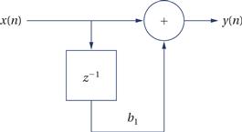
Figure 5.2 A signal flow graph.
Filters and buffering
The code to produce one FIR filter output looks like this:
for (i=0, y=0.0; i<N; i++)
y += x[i] * b[i];
However, the filter takes in a new sample on every sample period. The new input becomes x1 , the old x1 becomes x2 , etc. x0 is stored directly in the circular buffer but must be multiplied by b0 before being added to the output sum. Early digital filters were built-in hardware, where we can build a shift register to perform this operation. If we used an analogous operation in software, we would move every value in the filter on every sample period. We can avoid that with a circular buffer, moving the head without moving the data elements.
The next example uses our circular buffer class to build an FIR filter.
Programming Example 5.3 An FIR Filter in C
Here is a signal flow graph for an FIR filter:
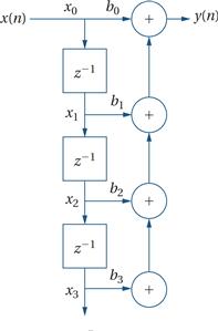
The delay elements running vertically hold the input samples with the most recent sample at the top and the oldest one at the bottom. Unfortunately, the signal flow graph doesn’t explicitly label all of the values that we use as inputs to operations, so the figure also shows the values (xi ) we need to operate on in our FIR loop.
When we compute the filter function, we want to match the bi’s and xi’s. We will use our circular buffer for the x’s, which change over time. We will use a standard array for the b’s, which don’t change. In order for the filter function to be able to use the same I value for both sets of data, we need to put the x data in the proper order. We can put the b data in a standard array with b0 being the first element. When we add a new x value, it becomes x 0 and replaces the oldest data value in the buffer. This means that the buffer head moves from higher to lower values, not lower to higher as we might expect.
Here is the modified version of circ_update() that puts a new sample into the buffer into the desired order:
void circ_update(int xnew) {
/* add the new sample and push off the oldest one */
/* compute the new head value with wraparound; the pos pointer moves from CMAX-1 down to 0 */
pos = ((pos == 0) ? CMAX-1 : (pos-1));
/* insert the new value at the new head */
circ[pos] = xnew;
}
We also need to change circ_init() to set pos = 0 initially. We don’t need to change circ_get();
Given these functions, the filter itself is simple. Here is our code for the FIR filter function:
int fir(int xnew) {
/* given a new sample value, update the queue and compute the filter output */
int i;
int result; /* holds the filter output */
circ_update(xnew); /* put the new value in */
for (i=0, result=0; i<CMAX; i++) /* compute the filter function */
result += b[i] * circ_get(i);
return result;
}
There is only one major structure for FIR filters but several for IIR filters, depending on the application requirements. One of the important reasons for so many different IIR forms is numerical properties—depending on the filter structure and coefficients, one structure may give significantly less numerical noise than another. But numerical noise is beyond the scope of our discussion so let’s concentrate on one form of IIR filter that highlights buffering issues. The next example looks at one form of IIR filter.
Programming Example 5.4 A Direct Form II IIR Filter Class in C
Here is what is known as the direct form II of an IIR filter:
This structure is designed to minimize the amount of buffer space required. Other forms of the IIR filter have other advantages but require more storage. We will store the vi values as in the FIR filter. In this case, v0 does not represent the input, but rather the left-hand sum. But v0 is stored before multiplication by b0 so that we can move v0 to v1 on the following sample period.
We can use the same circ_update() and circ_get() functions that we used for the FIR filter. We need two coefficient arrays, one for as and one for bs; as with the FIR filter, we can use standard C arrays for the coefficients because they don’t change over time. Here is the IIR filter function:
int iir2(int xnew) {
/* given a new sample value, update the queue and compute the filter output */
int i, aside, bside, result;
for (i=0, aside=0; i<ZMAX; i++)
aside += -a[i+1] * circ_get(i);
for (i=0, bside=0; i<ZMAX; i++)
bside += b[i+1] * circ_get(i);
result = b[0] * (xnew + aside) + bside;
circ_update(xnew); /* put the new value in */
return result;
}
5.2.3 Queues and Producer/Consumer Systems
Queues are also used in signal processing and event processing. Queues are used whenever data may arrive and depart at somewhat unpredictable times or when variable amounts of data may arrive. A queue is often referred to as an elastic buffer. We saw how to use elastic buffers for I/O in Chapter 3.
One way to build a queue is with a linked list. This approach allows the queue to grow to an arbitrary size. But in many applications we are unwilling to pay the price of dynamically allocating memory. Another way to design the queue is to use an array to hold all the data. Although some writers use both circular buffer and queue to mean the same thing, we use the term circular buffer to refer to a buffer that always has a fixed number of data elements while a queue may have varying numbers of elements in it.
Programming Example 5.5 gives C code for a queue that is built from an array.
Programming Example 5.5 An Array-Based Queue
The first step in designing the queue is to declare the array that we will use for the buffer:
#define Q_SIZE 5 /* your queue size may vary */
#define Q_MAX (Q_SIZE-1) /* this is the maximum index value into the array */
int q[Q_SIZE]; /* the array for our queue */
int head, tail; /* indexes for the current queue head and tail */
The variables head and tail keep track of the two ends of the queue.
Here is the initialization code for the queue:
void queue_init() {
/* initialize the queue data structure */
head = 0;
tail = 0;
}
We initialize the head and tail to the same position. As we add a value to the tail of the queue, we will increment tail. Similarly, when we remove a value from the head, we will increment head. The value of head is always equal to the location of the first element of the queue (except for when the queue is empty). The value of tail, in contrast, points to the location in which the next queue entry will go. When we reach the end of the array, we must wrap around these values—for example, when we add a value into the last element of q, the new value of tail becomes the 0th entry of the array.
We need to check for two error conditions: removing from an empty queue and adding to a full queue. In the first case, we know the queue is empty if head == tail. In the second case, we know the queue is full if incrementing tail will cause it to equal head. Testing for fullness, however, is a little harder because we have to worry about wraparound.
Here is the code for adding an element to the tail of the queue, which is known as enqueueing:
void enqueue(int val) {
/* check for a full queue */
if (((tail+1) % Q_SIZE) == head) error("enqueue onto full queue",tail);
/* add val to the tail of the queue */
q[tail] = val;
/* update the tail */
if (tail == Q_MAX)
tail = 0;
else
tail++;
}
And here is the code for removing an element from the head of the queue, known as dequeueing:
int dequeue() {
int returnval; /* use this to remember the value that you will return */
/* check for an empty queue */
if (head == tail) error("dequeue from empty queue",head);
/* remove from the head of the queue */
returnval = q[head];
/* update head */
if (head == Q_MAX)
head = 0;
else
head++;
/* return the value */
return returnval;
}
Digital filters always take in the same amount of data in each time period. Many systems, even signal processing systems, don’t fit that mold. Rather, they may take in varying amounts of data over time and produce varying amounts. When several of these systems operate in a chain, the variable-rate output of one stage becomes the variable-rate input of another stage.
Producer/consumer
Figure 5.3 shows a block diagram of a simple producer/consumer system. p1 and p2 are the two blocks that perform algorithmic processing. The data is fed to them by queues that act as elastic buffers. The queues modify the flow of control in the system as well as store data. If, for example, p2 runs ahead of p1, it will eventually run out of data in its q12 input queue. At that point, the queue will return an empty signal to p2. At this point, p2 should stop working until more data is available. This sort of complex control is easier to implement in a multitasking environment, as we will see in Chapter 6, but it is also possible to make effective use of queues in programs structured as nested procedures.
Figure 5.3 A producer/consumer system.
Data structures in queues
The queues in a producer/consumer may hold either uniform-sized data elements or variable-sized data elements. In some cases, the consumer needs to know how many of a given type of data element are associated together. The queue can be structured to hold a complex data type. Alternatively, the data structure can be stored as bytes or integers in the queue with, for example, the first integer holding the number of successive data elements.
5.3 Models of Programs
In this section, we develop models for programs that are more general than source code. Why not use the source code directly? First, there are many different types of source code—assembly languages, C code, and so on—but we can use a single model to describe all of them. Once we have such a model, we can perform many useful analyses on the model more easily than we could on the source code.
Our fundamental model for programs is the control/data flow graph (CDFG). (We can also model hardware behavior with the CDFG.) As the name implies, the CDFG has constructs that model both data operations (arithmetic and other computations) and control operations (conditionals). Part of the power of the CDFG comes from its combination of control and data constructs. To understand the CDFG, we start with pure data descriptions and then extend the model to control.
5.3.1 Data Flow Graphs
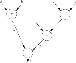
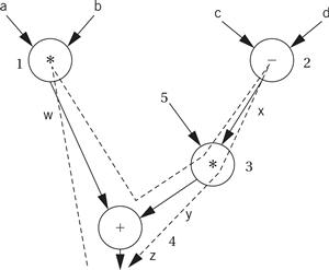
A data flow graph is a model of a program with no conditionals. In a high-level programming language, a code segment with no conditionals—more precisely, with only one entry and exit point—is known as a basic block. Figure 5.4 shows a simple basic block. As the C code is executed, we would enter this basic block at the beginning and execute all the statements.

Figure 5.4 A basic block in C.
Before we are able to draw the data flow graph for this code we need to modify it slightly. There are two assignments to the variable x—it appears twice on the left side of an assignment. We need to rewrite the code in single-assignment form, in which a variable appears only once on the left side. Because our specification is C code, we assume that the statements are executed sequentially, so that any use of a variable refers to its latest assigned value. In this case, x is not reused in this block (presumably it is used elsewhere), so we just have to eliminate the multiple assignment to x. The result is shown in Figure 5.5 where we have used the names x1 and x2 to distinguish the separate uses of x.

Figure 5.5 The basic block in single-assignment form.
The single-assignment form is important because it allows us to identify a unique location in the code where each named location is computed. As an introduction to the data flow graph, we use two types of nodes in the graph—round nodes denote operators and square nodes represent values. The value nodes may be either inputs to the basic block, such as a and b, or variables assigned to within the block, such as w and x1. The data flow graph for our single-assignment code is shown in Figure 5.6. The single-assignment form means that the data flow graph is acyclic—if we assigned to x multiple times, then the second assignment would form a cycle in the graph including x and the operators used to compute x. Keeping the data flow graph acyclic is important in many types of analyses we want to do on the graph. (Of course, it is important to know whether the source code actually assigns to a variable multiple times, because some of those assignments may be mistakes. We consider the analysis of source code for proper use of assignments in Section 5.5.)
Figure 5.6 An extended data flow graph for our sample basic block.
The data flow graph is generally drawn in the form shown in Figure 5.7. Here, the variables are not explicitly represented by nodes. Instead, the edges are labeled with the variables they represent. As a result, a variable can be represented by more than one edge. However, the edges are directed and all the edges for a variable must come from a single source. We use this form for its simplicity and compactness.
Figure 5.7 Standard data flow graph for our sample basic block.
The data flow graph for the code makes the order in which the operations are performed in the C code much less obvious. This is one of the advantages of the data flow graph. We can use it to determine feasible reorderings of the operations, which may help us to reduce pipeline or cache conflicts. We can also use it when the exact order of operations simply doesn’t matter. The data flow graph defines a partial ordering of the operations in the basic block. We must ensure that a value is computed before it is used, but generally there are several possible orderings of evaluating expressions that satisfy this requirement.
5.3.2 Control/Data Flow Graphs
A CDFG uses a data flow graph as an element, adding constructs to describe control. In a basic CDFG, we have two types of nodes: decision nodes and data flow nodes. A data flow node encapsulates a complete data flow graph to represent a basic block. We can use one type of decision node to describe all the types of control in a sequential program. (The jump/branch is, after all, the way we implement all those high-level control constructs.)
Figure 5.8 shows a bit of C code with control constructs and the CDFG constructed from it. The rectangular nodes in the graph represent the basic blocks. The basic blocks in the C code have been represented by function calls for simplicity. The diamond-shaped nodes represent the conditionals. The node’s condition is given by the label, and the edges are labeled with the possible outcomes of evaluating the condition.
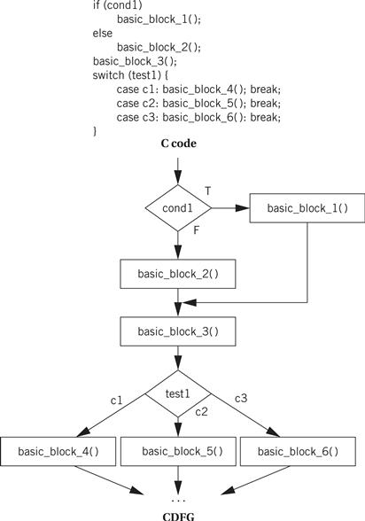
Figure 5.8 C code and its CDFG.
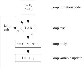
Building a CDFG for a while loop is straightforward, as shown in Figure 5.9. The while loop consists of both a test and a loop body, each of which we know how to represent in a CDFG. We can represent for loops by remembering that, in C, a for loop is defined in terms of a while loop. This for loop
for (i = 0; i < N; i++) {
loop_body();
}
is equivalent to
i = 0;
while (i < N) {
loop_body();
i++;
}
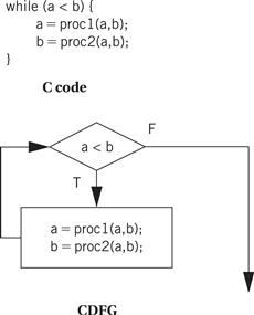
Figure 5.9 A while loop and its CDFG.
Hierarchical representation
For a complete CDFG model, we can use a data flow graph to model each data flow node. Thus, the CDFG is a hierarchical representation—a data flow CDFG can be expanded to reveal a complete data flow graph.
An execution model for a CDFG is very much like the execution of the program it represents. The CDFG does not require explicit declaration of variables but we assume that the implementation has sufficient memory for all the variables. We can define a state variable that represents a program counter in a CPU. (When studying a drawing of a CDFG, a finger works well for keeping track of the program counter state.) As we execute the program, we either execute the data flow node or compute the decision in the decision node and follow the appropriate edge, depending on the type of node the program counter points on. Even though the data flow nodes may specify only a partial ordering on the data flow computations, the CDFG is a sequential representation of the program. There is only one program counter in our execution model of the CDFG, and operations are not executed in parallel.
The CDFG is not necessarily tied to high-level language control structures. We can also build a CDFG for an assembly language program. A jump instruction corresponds to a nonlocal edge in the CDFG. Some architectures, such as ARM and many VLIW processors, support predicated execution of instructions, which may be represented by special constructs in the CDFG.
5.4 Assembly, Linking, and Loading
Assembly and linking are the last steps in the compilation process—they turn a list of instructions into an image of the program’s bits in memory. Loading actually puts the program in memory so that it can be executed. In this section, we survey the basic techniques required for assembly linking to help us understand the complete compilation and loading process.
Program generation work flow
Figure 5.10 highlights the role of assemblers and linkers in the compilation process. This process is often hidden from us by compilation commands that do everything required to generate an executable program. As the figure shows, most compilers do not directly generate machine code, but instead create the instruction-level program in the form of human-readable assembly language. Generating assembly language rather than binary instructions frees the compiler writer from details extraneous to the compilation process, which includes the instruction format as well as the exact addresses of instructions and data. The assembler’s job is to translate symbolic assembly language statements into bit-level representations of instructions known as object code. The assembler takes care of instruction formats and does part of the job of translating labels into addresses. However, because the program may be built from many files, the final steps in determining the addresses of instructions and data are performed by the linker, which produces an executable binary file. That file may not necessarily be located in the CPU’s memory, however, unless the linker happens to create the executable directly in RAM. The program that brings the program into memory for execution is called a loader.
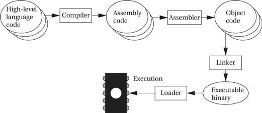
Figure 5.10 Program generation from compilation through loading.
Absolute and relative addresses
The simplest form of the assembler assumes that the starting address of the assembly language program has been specified by the programmer. The addresses in such a program are known as absolute addresses. However, in many cases, particularly when we are creating an executable out of several component files, we do not want to specify the starting addresses for all the modules before assembly—if we did, we would have to determine before assembly not only the length of each program in memory but also the order in which they would be linked into the program. Most assemblers therefore allow us to use relative addresses by specifying at the start of the file that the origin of the assembly language module is to be computed later. Addresses within the module are then computed relative to the start of the module. The linker is then responsible for translating relative addresses into addresses.
5.4.1 Assemblers
When translating assembly code into object code, the assembler must translate opcodes and format the bits in each instruction, and translate labels into addresses. In this section, we review the translation of assembly language into binary.
Labels make the assembly process more complex, but they are the most important abstraction provided by the assembler. Labels let the programmer (a human programmer or a compiler generating assembly code) avoid worrying about the locations of instructions and data. Label processing requires making two passes through the assembly source code:
1. The first pass scans the code to determine the address of each label.
2. The second pass assembles the instructions using the label values computed in the first pass.
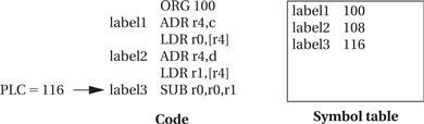
Symbol table
As shown in Figure 5.11, the name of each symbol and its address is stored in a symbol table that is built during the first pass. The symbol table is built by scanning from the first instruction to the last. (For the moment, we assume that we know the address of the first instruction in the program.) During scanning, the current location in memory is kept in a program location counter (PLC). Despite the similarity in name to a program counter, the PLC is not used to execute the program, only to assign memory locations to labels. For example, the PLC always makes exactly one pass through the program, whereas the program counter makes many passes over code in a loop. Thus, at the start of the first pass, the PLC is set to the program’s starting address and the assembler looks at the first line. After examining the line, the assembler updates the PLC to the next location (because ARM instructions are four bytes long, the PLC would be incremented by four) and looks at the next instruction. If the instruction begins with a label, a new entry is made in the symbol table, which includes the label name and its value. The value of the label is equal to the current value of the PLC. At the end of the first pass, the assembler rewinds to the beginning of the assembly language file to make the second pass. During the second pass, when a label name is found, the label is looked up in the symbol table and its value substituted into the appropriate place in the instruction.
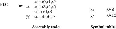
Figure 5.11 Symbol table processing during assembly.
But how do we know the starting value of the PLC? The simplest case is addressing. In this case, one of the first statements in the assembly language program is a pseudo-op that specifies the origin of the program, that is, the location of the first address in the program. A common name for this pseudo-op (e.g., the one used for the ARM) is the ORG statement
ORG 2000
which puts the start of the program at location 2000. This pseudo-op accomplishes this by setting the PLC’s value to its argument’s value, 2000 in this case. Assemblers generally allow a program to have many ORG statements in case instructions or data must be spread around various spots in memory.
Example 5.1 illustrates the use of the PLC in generating the symbol table.
Example 5.1 Generating a Symbol Table
Let’s use the following simple example of ARM assembly code:
ORG 100
label1 ADR r4,c
LDR r0,[r4]
label2 ADR r4,d
LDR r1,[r4]
label3 SUB r0,r0,r1
The initial ORG statement tells us the starting address of the program. To begin, let’s initialize the symbol table to an empty state and put the PLC at the initial ORG statement.
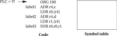
The PLC value shown is at the beginning of this step, before we have processed the ORG statement. The ORG tells us to set the PLC value to 100.
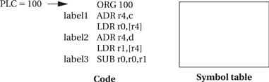
To process the next statement, we move the PLC to point to the next statement. But because the last statement was a pseudo-op that generates no memory values, the PLC value remains at 100.
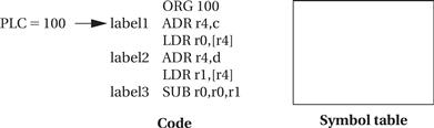
Because there is a label in this statement, we add it to the symbol table, taking its value from the current PLC value.
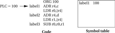
To process the next statement, we advance the PLC to point to the next line of the program and increment its value by the length in memory of the last line, namely, 4.
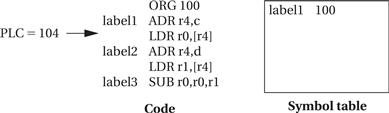
We continue this process as we scan the program until we reach the end, at which the state of the PLC and symbol table are as shown below.
Assemblers allow labels to be added to the symbol table without occupying space in the program memory. A typical name of this pseudo-op is EQU for equate. For example, in the code
ADD r0,r1,r2
FOO EQU 5
BAZ SUB r3,r4,#FOO
the EQU pseudo-op adds a label named FOO with the value 5 to the symbol table. The value of the BAZ label is the same as if the EQU pseudo-op were not present, because EQU does not advance the PLC. The new label is used in the subsequent SUB instruction as the name for a constant. EQUs can be used to define symbolic values to help make the assembly code more structured.
ARM ADR pseudo-op
The ARM assembler supports one pseudo-op that is particular to the ARM instruction set. In other architectures, an address would be loaded into a register (e.g., for an indirect access) by reading it from a memory location. ARM does not have an instruction that can load an effective address, so the assembler supplies the ADR pseudo-op to create the address in the register. It does so by using ADD or SUB instructions to generate the address. The address to be loaded can be register relative, program relative, or numeric, but it must assemble to a single instruction. More complicated address calculations must be explicitly programmed.
Object code formats
The assembler produces an object file that describes the instructions and data in binary format. A commonly used object file format, originally developed for Unix but now used in other environments as well, is known as COFF (common object file format). The object file must describe the instructions, data, and any addressing information and also usually carries along the symbol table for later use in debugging.
Generating relative code rather than code introduces some new challenges to the assembly language process. Rather than using an ORG statement to provide the starting address, the assembly code uses a pseudo-op to indicate that the code is in fact relocatable. (Relative code is the default for the ARM assembler.) Similarly, we must mark the output object file as being relative code. We can initialize the PLC to 0 to denote that addresses are relative to the start of the file. However, when we generate code that makes use of those labels, we must be careful, because we do not yet know the actual value that must be put into the bits. We must instead generate relocatable code. We use extra bits in the object file format to mark the relevant fields as relocatable and then insert the label’s relative value into the field. The linker must therefore modify the generated code—when it finds a field marked as relative, it uses the addresses that it has generated to replace the relative value with a correct, value for the address. To understand the details of turning relocatable code into executable code, we must understand the linking process described in the next section.
5.4.2 Linking
Many assembly language programs are written as several smaller pieces rather than as a single large file. Breaking a large program into smaller files helps delineate program modularity. If the program uses library routines, those will already be preassembled, and assembly language source code for the libraries may not be available for purchase. A linker allows a program to be stitched together out of several smaller pieces. The linker operates on the object files created by the assembler and modifies the assembled code to make the necessary links between files.
Some labels will be both defined and used in the same file. Other labels will be defined in a single file but used elsewhere as illustrated in Figure 5.12. The place in the file where a label is defined is known as an entry point. The place in the file where the label is used is called an external reference. The main job of the loader is to resolve external references based on available entry points. As a result of the need to know how definitions and references connect, the assembler passes to the linker not only the object file but also the symbol table. Even if the entire symbol table is not kept for later debugging purposes, it must at least pass the entry points. External references are identified in the object code by their relative symbol identifiers.
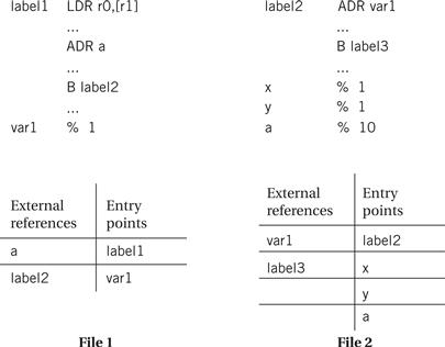
Figure 5.12 External references and entry points.
Linking process
The linker proceeds in two phases. First, it determines the address of the start of each object file. The order in which object files are to be loaded is given by the user, either by specifying parameters when the loader is run or by creating a load map file that gives the order in which files are to be placed in memory. Given the order in which files are to be placed in memory and the length of each object file, it is easy to compute the starting address of each file. At the start of the second phase, the loader merges all symbol tables from the object files into a single, large table. It then edits the object files to change relative addresses into addresses. This is typically performed by having the assembler write extra bits into the object file to identify the instructions and fields that refer to labels. If a label cannot be found in the merged symbol table, it is undefined and an error message is sent to the user.
Controlling where code modules are loaded into memory is important in embedded systems. Some data structures and instructions, such as those used to manage interrupts, must be put at precise memory locations for them to work. In other cases, different types of memory may be installed at different address ranges. For example, if we have flash in some locations and DRAM in others, we want to make sure that locations to be written are put in the DRAM locations.
Dynamically linked libraries
Workstations and PCs provide dynamically linked libraries, and certain sophisticated embedded computing environments may provide them as well. Rather than link a separate copy of commonly used routines such as I/O to every executable program on the system, dynamically linked libraries allow them to be linked in at the start of program execution. A brief linking process is run just before execution of the program begins; the dynamic linker uses code libraries to link in the required routines. This not only saves storage space but also allows programs that use those libraries to be easily updated. However, it does introduce a delay before the program starts executing.
5.4.3 Object Code Design
We have to take several issues into account when designing object code. In a timesharing system, many of these details are taken care of for us. When designing an embedded system, we may need to handle some of them ourselves.
Memory map design
As we saw, the linker allows us to control where object code modules are placed in memory. We may need to control the placement of several types of data:
• Interrupt vectors and other information for I/O devices must be placed in specific locations.
• Memory management tables must be set up.
• Global variables used for communication between processes must be put in locations that are accessible to all the users of that data.
We can give these locations symbolic names so that, for example, the same software can work on different processors that put these items at different addresses. But the linker must be given the proper absolute addresses to configure the program’s memory.
Reentrancy
Many programs should be designed to be reentrant. A program is reentrant if can be interrupted by another call to the function without changing the results of either call. If the program changes the value of global variables, it may give a different answer when it is called recursively. Consider this code:
int foo = 1;
int task1() {
foo = foo + 1;
return foo;
}
In this simple example, the variable foo is modified and so task1() gives a different answer on every invocation. We can avoid this problem by passing foo in as an argument:
int task1(int foo) {
return foo+1;
}
Relocatability
A program is relocatable if it can be executed when loaded into different parts of memory. Relocatability requires some sort of support from hardware that provides address calculation. But it is possible to write nonrelocatable code for nonrelocatable architectures. In some cases, it may be necessary to use a nonrelocatable address, such as when addressing an I/O device. However, any addresses that are not fixed by the architecture or system configuration should be accessed using relocatable code.
5.5 Compilation Techniques
Even though we don’t write our own assembly code much of the time, we still care about the characteristics of the code our compiler generates: its speed, its size, and its power consumption. Understanding how a compiler works will help us write code and direct the compiler to get the assembly language implementation we want. We will start with an overview of the compilation process, then some basic compilation methods, and conclude with some more advanced optimizations.
5.5.1 The Compilation Process
It is useful to understand how a high-level language program is translated into instructions: interrupt handling instructions, placement of data and instructions in memory, etc. Understanding how the compiler works can help you know when you cannot rely on the compiler. Next, because many applications are also performance sensitive, understanding how code is generated can help you meet your performance goals, either by writing high-level code that gets compiled into the instructions you want or by recognizing when you must write your own assembly code.
We can summarize the compilation process with a formula:

The high-level language program is translated into the lower-level form of instructions; optimizations try to generate better instruction sequences than would be possible if the brute force technique of independently translating source code statements were used. Optimization techniques focus on more of the program to ensure that compilation decisions that appear to be good for one statement are not unnecessarily problematic for other parts of the program.
The compilation process is outlined in Figure 5.13. Compilation begins with high-level language code such as C or C++ and generally produces assembly code. (Directly producing object code simply duplicates the functions of an assembler, which is a very desirable stand-alone program to have.) The high-level language program is parsed to break it into statements and expressions. In addition, a symbol table is generated, which includes all the named objects in the program. Some compilers may then perform higher-level optimizations that can be viewed as modifying the high-level language program input without reference to instructions.
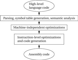
Figure 5.13 The compilation process.
Simplifying arithmetic expressions is one example of a machine-independent optimization. Not all compilers do such optimizations, and compilers can vary widely regarding which combinations of machine-independent optimizations they do perform. Instruction-level optimizations are aimed at generating code. They may work directly on real instructions or on a pseudo-instruction format that is later mapped onto the instructions of the target CPU. This level of optimization also helps modularize the compiler by allowing code generation to create simpler code that is later optimized. For example, consider this array access code:
x[i] = c*x[i];
A simple code generator would generate the address for x[i] twice, once for each appearance in the statement. The later optimization phases can recognize this as an example of common expressions that need not be duplicated. While in this simple case it would be possible to create a code generator that never generated the redundant expression, taking into account every such optimization at code generation time is very difficult. We get better code and more reliable compilers by generating simple code first and then optimizing it.
5.5.2 Basic Compilation Methods
Statement translation
In this section, we consider the basic job of translating the high-level language program with little or no optimization. Let’s first consider how to translate an expression. A large amount of the code in a typical application consists of arithmetic and logical expressions. Understanding how to compile a single expression, as described in the next example, is a good first step in understanding the entire compilation process.
Example 5.2 Compiling an Arithmetic Expression
Consider this arithmetic expression:
x = a*b + 5*(c − d)
The expression is written in terms of program variables. In some machines we may be able to perform memory-to-memory arithmetic directly on the locations corresponding to those variables. However, in many machines, such as the ARM, we must first load the variables into registers. This requires choosing which registers receive not only the named variables but also intermediate results such as (c − d).
The code for the expression can be built by walking the data flow graph. Here is the data flow graph for the expression.
The temporary variables for the intermediate values and final result have been named w, x, y, and z. To generate code, we walk from the tree’s root (where z, the final result, is generated) by traversing the nodes in post order. During the walk, we generate instructions to cover the operation at every node. Here is the path:
The nodes are numbered in the order in which code is generated. Because every node in the data flow graph corresponds to an operation that is directly supported by the instruction set, we simply generate an instruction at every node. Because we are making an arbitrary register assignment, we can use up the registers in order starting with r1. Here is the resulting ARM code:
; operator 1 (+)
ADR r4,a ; get address for a
MOV r1,[r4] ; load a
ADR r4,b ; get address for b
MOV r2,[r4] ; load b
ADD r3,r1,r2 ; put w into r3
; operator 2 (−)
ADR r4,c ; get address for c
MOV r4,[r4] ; load c
ADR r4,d ; get address for d
MOV r5,[r4] ; load d
SUB r6,r4,r5 ; put z into r6
; operator 3 (*)
MUL r7,r6,#5 ; operator 3, puts y into r7
; operator 4 (+)
ADD r8,r7,r3 ; operator 4, puts x into r8
; assign to x
ADR r1,x
STR r8,[r1] ; assigns to x location
One obvious optimization is to reuse a register whose value is no longer needed. In the case of the intermediate values w, y, and z, we know that they cannot be used after the end of the expression (e.g., in another expression) because they have no name in the C program. However, the final result z may in fact be used in a C assignment and the value reused later in the program. In this case we would need to know when the register is no longer needed to determine its best use.
For comparison, here is the code generated by the ARM gcc compiler with handwritten comments:
ldr r2, [fp, #−16]
ldr r3, [fp, #−20]
mul r1, r3, r2 ; multiply
ldr r2, [fp, #−24]
ldr r3, [fp, #−28]
rsb r2, r3, r2 ; subtract
mov r3, r2
mov r3, r3, asl #2
add r3, r3, r2 ; add
add r3, r1, r3 ; add
str r3, [fp, #−32] ; assign
In the previous example, we made an arbitrary allocation of variables to registers for simplicity. When we have large programs with multiple expressions, we must allocate registers more carefully because CPUs have a limited number of registers. We will consider register allocation in more detail below.
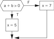
We also need to be able to translate control structures. Because conditionals are controlled by expressions, the code generation techniques of the last example can be used for those expressions, leaving us with the task of generating code for the flow of control itself. Figure 5.14 shows a simple example of changing flow of control in C—an if statement, in which the condition controls whether the true or false branch of the if is taken. Figure 5.14 also shows the control flow diagram for the if statement.
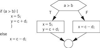
Figure 5.14 Flow of control in C and control flow diagrams.
The next example illustrates how to implement conditionals in assembly language.
Example 5.3 Generating Code for a Conditional
Consider this C statement:
if (a + b > 0)
x = 5;
else
x = 7;
The CDFG for the statement appears below.
We know how to generate the code for the expressions. We can generate the control flow code by walking the CDFG. One ordered walk through the CDFG follows:
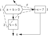
To generate code, we must assign a label to the first instruction at the end of a directed edge and create a branch for each edge that does not go to the immediately following instruction. The exact steps to be taken at the branch points depend on the target architecture. On some machines, evaluating expressions generates condition codes that we can test in subsequent branches, and on other machines we must use test-and-branch instructions. ARM allows us to test condition codes, so we get the following ARM code for the 1-2-3 walk:
ADR r5,a ; get address for a
LDR r1,[r5] ; load a
ADR r5,b ; get address for b
LDR r2,b ; load b
ADD r3,r1,r2
BLE label3 ; true condition falls through branch
; true case
LDR r3,#5 ; load constant
ADR r5,x
STR r3, [r5] ; store value into x
B stmtend ; done with the true case
; false case
label3 LDR r3,#7 ; load constant
ADR r5,x ; get address of x
STR r3,[r5] ; store value into x
stmtend …
The 1-2 and 3-4 edges do not require a branch and label because they are straight-line code. In contrast, the 1-3 and 2-4 edges do require a branch and a label for the target.
For comparison, here is the code generated by the ARM gcc compiler with some handwritten comments:
ldr r2, [fp, #−16]
ldr r3, [fp, #−20]
add r3, r2, r3
cmp r3, #0 ; test the branch condition
ble .L3 ; branch to false block if < =
mov r3, #5 ; true block
str r3, [fp, #−32]
b .L4 ; go to end of if statement
.L3: ; false block
mov r3, #7
str r3, [fp, #−32]
.L4:
Because expressions are generally created as straight-line code, they typically require careful consideration of the order in which the operations are executed. We have much more freedom when generating conditional code because the branches ensure that the flow of control goes to the right block of code. If we walk the CDFG in a different order and lay out the code blocks in a different order in memory, we still get valid code as long as we properly place branches.
Drawing a control flow graph based on the while form of the loop helps us understand how to translate it into instructions.
C compilers can generate (using the -s flag) assembler source, which some compilers intersperse with the C code. Such code is a very good way to learn about both assembly language programming and compilation.
Procedures
Another major code generation problem is the creation of procedures. Generating code for procedures is relatively straightforward once we know the procedure linkage appropriate for the CPU. At the procedure definition, we generate the code to handle the procedure call and return. At each call of the procedure, we set up the procedure parameters and make the call.
The CPU’s subroutine call mechanism is usually not sufficient to directly support procedures in modern programming languages. We introduced the procedure stack and procedure linkages in Chapter 2. The linkage mechanism provides a way for the program to pass parameters into the program and for the procedure to return a value. It also provides help in restoring the values of registers that the procedure has modified. All procedures in a given programming language use the same linkage mechanism (although different languages may use different linkages). The mechanism can also be used to call handwritten assembly language routines from compiled code.
Procedure stacks are typically built to grow down from high addresses. A stack pointer (sp) defines the end of the current frame, while a frame pointer (fp) defines the end of the last frame. (The fp is technically necessary only if the stack frame can be grown by the procedure during execution.) The procedure can refer to an element in the frame by addressing relative to sp. When a new procedure is called, the sp and fp are modified to push another frame onto the stack.
As we saw in Chapter 2, the ARM Procedure Call Standard (APCS) [Slo04] is the recommended procedure linkage for ARM processors. r0–r3 are used to pass the first four parameters into the procedure. r0 is also used to hold the return value.
The next example looks at compiler-generated procedure linkage code.
Example 5.4 Procedure Linkage in C
Here is a procedure definition:
int p1(int a, int b, int c, int d, int e) {
return a + e;
}
This procedure has five parameters, so we would expect that one of them would be passed through the stack while the rest are passed through registers. It also returns an integer value, which should be returned in r0. Here is the code for the procedure generated by the ARM gcc compiler with some handwritten comments:
mov ip, sp ; procedure entry
stmfd sp!, {fp, ip, lr, pc}
sub fp, ip, #4
sub sp, sp, #16
str r0, [fp, #−16] ; put first four args on stack
str r1, [fp, #−20]
str r2, [fp, #−24]
str r3, [fp, #−28]
ldr r2, [fp, #−16] ; load a
ldr r3, [fp, #4] ; load e
add r3, r2, r3 ; compute a + e
mov r0, r3 ; put the result into r0 for return
ldmea fp, {fp, sp, pc} ; return
Here is a call to that procedure:
y = p1(a,b,c,d,x);
Here is the ARM gcc code with handwritten comments:
ldr r3, [fp, #−32] ; get e
str r3, [sp, #0] ; put into p1()’s stack frame
ldr r0, [fp, #−16] ; put a into r0
ldr r1, [fp, #−20] ; put b into r1
ldr r2, [fp, #−24] ; put c into r2
ldr r3, [fp, #−28] ; put d into r3
bl p1 ; call p1()
mov r3, r0 ; move return value into r3
str r3, [fp, #−36] ; store into y in stack frame
We can see that the compiler sometimes makes additional register moves but it does follow the ACPS standard.
Data structures
The compiler must also translate references to data structures into references to raw memories. In general, this requires address computations. Some of these computations can be done at compile time while others must be done at run time.
Arrays are interesting because the address of an array element must in general be computed at run time, because the array index may change. Let us first consider a one-dimensional array:
a[i]
The layout of the array in memory is shown in Figure 5.15: the zeroth element is stored as the first element of the array, the first element directly below, and so on. We can create a pointer for the array that points to the array’s head, namely, a[0]. If we call that pointer aptr for convenience, then we can rewrite the reading of a[i] as
*(aptr + i)
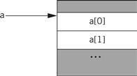
Figure 5.15 Layout of a one-dimensional array in memory.
Two-dimensional arrays are more challenging. There are multiple possible ways to lay out a two-dimensional array in memory, as shown in Figure 5.15. In this form, which is known as row major, the inner variable of the array (j in a[i,j]) varies most quickly. (Fortran uses a different organization known as column major.) Two-dimensional arrays also require more sophisticated addressing—in particular, we must know the size of the array. Let us consider the row-major form. If the a[] array is of size N × M, then we can turn the two-dimensional array access into a one-dimensional array access. Thus,
a[i,j]
becomes
a[i*M + j]
where the maximum value for j is M − 1.
A C struct is easier to address. As shown in Figure 5.16, a structure is implemented as a contiguous block of memory. Fields in the structure can be accessed using constant offsets to the base address of the structure. In this example, if field1 is four bytes long, then field2 can be accessed as
*(aptr + 4)
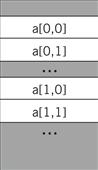
Figure 5.16 Memory layout for two-dimensional arrays.
This addition can usually be done at compile time, requiring only the indirection itself to fetch the memory location during execution.
5.5.3 Compiler Optimizations
Basic compilation techniques can generate inefficient code. Compilers use a wide range of algorithms to optimize the code they generate.
Loop transformations
Loops are important program structures—although they are compactly described in the source code, they often use a large fraction of the computation time. Many techniques have been designed to optimize loops.
A simple but useful transformation is known as loop unrolling, illustrated in the next example. Loop unrolling is important because it helps expose parallelism that can be used by later stages of the compiler.
Example 5.5 Loop Unrolling
Here is a simple C loop:
for (i = 0; i < N; i++) {
a[i]=b[i]*c[i];
}
This loop is executed a fixed number of times, namely, N. A straightforward implementation of the loop would create and initialize the loop variable i, update its value on every iteration, and test it to see whether to exit the loop. However, because the loop is executed a fixed number of times, we can generate more direct code.
If we let N = 4, then we can substitute this straight-line code for the loop:
a[0] = b[0]*c[0];
a[1] = b[1]*c[1];
a[2] = b[2]*c[2];
a[3] = b[3]*c[3];
This unrolled code has no loop overhead code at all, that is, no iteration variable and no tests. But the unrolled loop has the same problems as the inlined procedure—it may interfere with the cache and expands the amount of code required.
We do not, of course, have to fully unroll loops. Rather than unroll the above loop four times, we could unroll it twice. Unrolling produces this code:
for (i = 0; i < 2; i++) {
a[i*2] = b[i*2]*c[i*2];
a[i*2 + 1] = b[i*2 + 1]*c[i*2 + 1];
}
In this case, because all operations in the two lines of the loop body are independent, later stages of the compiler may be able to generate code that allows them to be executed efficiently on the CPU’s pipeline.
Loop fusion combines two or more loops into a single loop. For this transformation to be legal, two conditions must be satisfied. First, the loops must iterate over the same values. Second, the loop bodies must not have dependencies that would be violated if they are executed together—for example, if the second loop’s ith iteration depends on the results of the i + 1th iteration of the first loop, the two loops cannot be combined. Loop distribution is the opposite of loop fusion, that is, decomposing a single loop into multiple loops.
Loop tiling breaks up a loop into a set of nested loops, with each inner loop performing the operations on a subset of the data. An example is shown in Figure 5.17. Here, each loop is broken up into tiles of size two. Each loop is split into two loops—for example, the inner ii loop iterates within the tile and the outer i loop iterates across the tiles. The result is that the pattern of accesses across the a array is drastically different—rather than walking across one row in its entirety, the code walks through rows and columns following the tile structure. Loop tiling changes the order in which array elements are accessed, thereby allowing us to better control the behavior of the cache during loop execution.
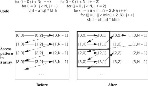
Figure 5.17 Loop tiling.
We can also modify the arrays being indexed in loops. Array padding adds dummy data elements to a loop in order to change the layout of the array in the cache. Although these array locations will not be used, they do change how the useful array elements fall into cache lines. Judicious padding can in some cases significantly reduce the number of cache conflicts during loop execution.
Dead code elimination
Dead code is code that can never be executed. Dead code can be generated by programmers, either inadvertently or purposefully. Dead code can also be generated by compilers. Dead code can be identified by reachability analysis—finding the other statements or instructions from which it can be reached. If a given piece of code cannot be reached, or it can be reached only by a piece of code that is unreachable from the main program, then it can be eliminated. Dead code elimination analyzes code for reachability and trims away dead code.
Register allocation
Register allocation is a very important compilation phase. Given a block of code, we want to choose assignments of variables (both declared and temporary) to registers to minimize the total number of required registers.
The next example illustrates the importance of proper register allocation.
Example 5.6 Register Allocation
To keep the example small, we assume that we can use only four of the ARM’s registers. In fact, such a restriction is not unthinkable—programming conventions can reserve certain registers for special purposes and significantly reduce the number of general-purpose registers available.
Consider this C code:
w = a + b; /* statement 1 */
x = c + w; /* statement 2 */
y = c + d; /* statement 3 */
A naive register allocation, assigning each variable to a separate register, would require seven registers for the seven variables in the above code. However, we can do much better by reusing a register once the value stored in the register is no longer needed. To understand how to do this, we can draw a lifetime graph that shows the statements on which each statement is used. Here is a lifetime graph in which the x axis is the statement number in the C code and the y axis shows the variables.
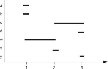
A horizontal line stretches from the first statement where the variable is used to the last use of the variable; a variable is said to be live during this interval. At each statement, we can determine every variable currently in use. The maximum number of variables in use at any statement determines the maximum number of registers required. In this case, statement two requires three registers: c, w, and x. This fits within the four-register limitation. By reusing registers once their current values are no longer needed, we can write code that requires no more than four registers. Here is one register assignment:
| a | r0 |
| b | r1 |
| c | r2 |
| d | r0 |
| w | r3 |
| x | r0 |
| y | r3 |
Here is the ARM assembly code that uses the above register assignment:
LDR r0,[p_a] ; load a into r0 using pointer to a (p_a)
LDR r1,[p_b] ; load b into r1
ADD r3,r0,r1 ; compute a + b
STR r3,[p_w] ; w = a + b
LDR r2,[p_c] ; load c into r2
ADD r0,r2,r3 ; compute c + w, reusing r0 for x
STR r0,[p_x] ; x = c + w
LDR r0,[p_d] ; load d into r0
ADD r3,r2,r0 ; compute c + d, reusing r3 for y
STR r3,[p_y] ; y = c + d
If a section of code requires more registers than are available, we must spill some of the values out to memory temporarily. After computing some values, we write the values to temporary memory locations, reuse those registers in other computations, and then reread the old values from the temporary locations to resume work. Spilling registers is problematic in several respects: it requires extra CPU time and uses up both instruction and data memory. Putting effort into register allocation to avoid unnecessary register spills is worth your time.
We can solve register allocation problems by building a conflict graph and solving a graph coloring problem. As shown in Figure 5.18, each variable in the high-level language code is represented by a node. An edge is added between two nodes if they are both live at the same time. The graph coloring problem is to use the smallest number of distinct colors to color all the nodes such that no two nodes are directly connected by an edge of the same color. The figure shows a satisfying coloring that uses three colors. Graph coloring is NP-complete, but there are efficient heuristic algorithms that can give good results on typical register allocation problems.
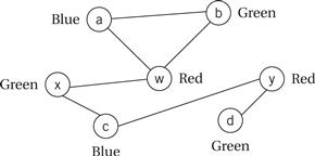
Figure 5.18 Using graph coloring to solve the problem of Example 5.6.
Lifetime analysis assumes that we have already determined the order in which we will evaluate operations. In many cases, we have freedom in the order in which we do things. Consider this expression:
(a + b) * (c − d)
We have to do the multiplication last, but we can do either the addition or the subtraction first. Different orders of loads, stores, and arithmetic operations may also result in different execution times on pipelined machines. If we can keep values in registers without having to reread them from main memory, we can save execution time and reduce code size as well.
The next example shows how proper operator scheduling can improve register allocation.
Example 5.7 Operator Scheduling for Register Allocation
Here is a sample C code fragment:
w = a + b; /* statement 1 */
x = c + d; /* statement 2 */
y = x + e; /* statement 3 */
z = a − b; /* statement 4 */
If we compile the statements in the order in which they were written, we get this register graph:
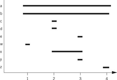
Because w is needed until the last statement, we need five registers at statement 3, even though only three registers are needed for the statement at line 3. If we swap statements 3 and 4 (renumbering them 39 and 49), we reduce our requirements to three registers. Here is the modified C code:
w = a + b; /* statement 1 */
z = a − b; /* statement 29 */
x = c + d; /* statement 39 */
y = x + e; /* statement 49 */
And here is the lifetime graph for the new code:
Compare the ARM assembly code for the two code fragments. We have written both assuming that we have only four free registers. In the before version, we do not have to write out any values, but we must read a and b twice. The after version allows us to retain all values in registers as long as we need them.
Before version After version
LDR r0,a LDR r0,a
LDR r1,b LDR r1,b
ADD r2,r0,r1 ADD r2,r1,r0
STR r2,w ; w = a + b STR r2,w ; w = a + b
LDRr r0,c SUB r2,r0,r1
LDR r1,d STR r2,z ; z = a − b
ADD r2,r0,r1 LDR r0,c
STR r2,x ; x = c + d LDR r1,d
LDR r1,e ADD r2,r1,r0
ADD r0,r1,r2 STR r2,x ; x = c + d
STR r0,y ; y = x + e LDR r1,e
LDR r0,a ; reload a ADD r0,r1,r2
LDR r1,b ; reload b STR r0,y ; y = x + e
SUB r2,r1,r0
STR r2,z ; z = a − b
Scheduling
We have some freedom to choose the order in which operations will be performed. We can use this to our advantage—for example, we may be able to improve the register allocation by changing the order in which operations are performed, thereby changing the lifetimes of the variables.
We can solve scheduling problems by keeping track of resource utilization over time. We do not have to know the exact microarchitecture of the CPU—all we have to know is that, for example, instruction types 1 and 2 both use resource A while instruction types 3 and 4 use resource B. CPU manufacturers generally disclose enough information about the microarchitecture to allow us to schedule instructions even when they do not provide a detailed description of the CPU’s internals.
We can keep track of CPU resources during instruction scheduling using a reservation table[Kog81]. As illustrated in Figure 5.19, rows in the table represent instruction execution time slots and columns represent resources that must be scheduled. Before scheduling an instruction to be executed at a particular time, we check the reservation table to determine whether all resources needed by the instruction are available at that time. Upon scheduling the instruction, we update the table to note all resources used by that instruction. Various algorithms can be used for the scheduling itself, depending on the types of resources and instructions involved, but the reservation table provides a good summary of the state of an instruction scheduling problem in progress.
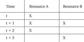
Figure 5.19 A reservation table for instruction scheduling.
We can also schedule instructions to maximize performance. As we know from Section 3.6, when an instruction that takes more cycles than normal to finish is in the pipeline, pipeline bubbles appear that reduce performance. Software pipelining is a technique for reordering instructions across several loop iterations to reduce pipeline bubbles. Some instructions take several cycles to complete; if the value produced by one of these instructions is needed by other instructions in the loop iteration, then they must wait for that value to be produced. Rather than pad the loop with no-ops, we can start instructions from the next iteration. The loop body then contains instructions that manipulate values from several different loop iterations—some of the instructions are working on the early part of iteration n + 1, others are working on iteration n, and still others are finishing iteration n − 1.
Instruction selection
Selecting the instructions to use to implement each operation is not trivial. There may be several different instructions that can be used to accomplish the same goal, but they may have different execution times. Moreover, using one instruction for one part of the program may affect the instructions that can be used in adjacent code. Although we can’t discuss all the problems and methods for code generation here, a little bit of knowledge helps us envision what the compiler is doing.
One useful technique for generating code is template matching, illustrated in Figure 5.20. We have a DAG that represents the expression for which we want to generate code. In order to be able to match up instructions and operations, we represent instructions using the same DAG representation. We shaded the instruction template nodes to distinguish them from code nodes. Each node has a cost, which may be simply the execution time of the instruction or may include factors for size, power consumption, and so on. In this case, we have shown that each instruction takes the same amount of time, and thus all have a cost of 1. Our goal is to cover all nodes in the code DAG with instruction DAGs—until we have covered the code DAG we haven’t generated code for all the operations in the expression. In this case, the lowest-cost covering uses the multiply-add instruction to cover both nodes. If we first tried to cover the bottom node with the multiply instruction, we would find ourselves blocked from using the multiply-add instruction. Dynamic programming can be used to efficiently find the lowest-cost covering of trees, and heuristics can extend the technique to DAGs.
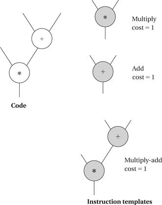
Figure 5.20 Code generation by template matching.
Understanding your compiler
Clearly, the compiler can vastly transform your program during the creation of assembly language. But compilers are also substantially different in terms of the optimizations they perform. Understanding your compiler can help you get the best code out of it.
Studying the assembly language output of the compiler is a good way to learn about what the compiler does. Some compilers will annotate sections of code to help you make the correspondence between the source and assembler output. Starting with small examples that exercise only a few types of statements will help. You can experiment with different optimization levels (the -O flag on most C compilers). You can also try writing the same algorithm in several ways to see how the compiler’s output changes.
If you can’t get your compiler to generate the code you want, you may need to write your own assembly language. You can do this by writing it from scratch or modifying the output of the compiler. If you write your own assembly code, you must ensure that it conforms to all compiler conventions, such as procedure call linkage. If you modify the compiler output, you should be sure that you have the algorithm right before you start writing code so that you don’t have to repeatedly edit the compiler’s assembly language output. You also need to clearly document the fact that the high-level language source is, in fact, not the code used in the system.
5.6 Program-Level Performance Analysis
Because embedded systems must perform functions in real time, we often need to know how fast a program runs. The techniques we use to analyze program execution time are also helpful in analyzing properties such as power consumption. In this section, we study how to analyze programs to estimate their run times. We also examine how to optimize programs to improve their execution times; of course, optimization relies on analysis.
It is important to keep in mind that CPU performance is not judged in the same way as program performance. Certainly, CPU clock rate is a very unreliable metric for program performance. But more importantly, the fact that the CPU executes part of our program quickly doesn’t mean that it will execute the entire program at the rate we desire. As illustrated in Figure 5.21, the CPU pipeline and cache act as windows into our program. In order to understand the total execution time of our program, we must look at execution paths, which in general are far longer than the pipeline and cache windows. The pipeline and cache influence execution time, but execution time is a global property of the program.
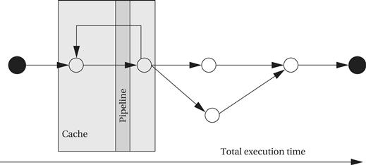
Figure 5.21 Execution time is a global property of a program.
While we might hope that the execution time of programs could be precisely determined, this is in fact difficult to do in practice:
• The execution time of a program often varies with the input data values because those values select different execution paths in the program. For example, loops may be executed a varying number of times, and different branches may execute blocks of varying complexity.
• The cache has a major effect on program performance, and once again, the cache’s behavior depends in part on the data values input to the program.
• Execution times may vary even at the instruction level. Floating-point operations are the most sensitive to data values, but the normal integer execution pipeline can also introduce data-dependent variations. In general, the execution time of an instruction in a pipeline depends not only on that instruction but on the instructions around it in the pipeline.
Measuring execution speed
We can measure program performance in several ways:
• Some microprocessor manufacturers supply simulators for their CPUs. The simulator runs on a workstation or PC, takes as input an executable for the microprocessor along with input data, and simulates the execution of that program. Some of these simulators go beyond functional simulation to measure the execution time of the program. Simulation is clearly slower than executing the program on the actual microprocessor, but it also provides much greater visibility during execution. Be careful—some microprocessor performance simulators are not 100% accurate, and simulation of I/O-intensive code may be difficult.
• A timer connected to the microprocessor bus can be used to measure performance of executing sections of code. The code to be measured would reset and start the timer at its start and stop the timer at the end of execution. The length of the program that can be measured is limited by the accuracy of the timer.
• A logic analyzer can be connected to the microprocessor bus to measure the start and stop times of a code segment. This technique relies on the code being able to produce identifiable events on the bus to identify the start and stop of execution. The length of code that can be measured is limited by the size of the logic analyzer’s buffer.
We are interested in the following three different types of performance measures on programs:
• average-case execution time: This is the typical execution time we would expect for typical data. Clearly, the first challenge is defining typicalinputs.
• worst-case execution time: The longest time that the program can spend on any input sequence is clearly important for systems that must meet deadlines. In some cases, the input set that causes the worst-case execution time is obvious, but in many cases it is not.
• best-case execution time: This measure can be important in multirate real-time systems, as seen in Chapter 6.
First, we look at the fundamentals of program performance in more detail. We then consider trace-driven performance based on executing the program and observing its behavior.
5.6.1 Elements of Program Performance
The key to evaluating execution time is breaking the performance problem into parts. Program execution time [Sha89] can be seen as

The path is the sequence of instructions executed by the program (or its equivalent in the high-level language representation of the program). The instruction timing is determined based on the sequence of instructions traced by the program path, which takes into account data dependencies, pipeline behavior, and caching. Luckily, these two problems can be solved relatively independently.
Although we can trace the execution path of a program through its high-level language specification, it is hard to get accurate estimates of total execution time from a high-level language program. This is because there is not a direct correspondence between program statements and instructions. The number of memory locations and variables must be estimated, and results may be either saved for reuse or recomputed on the fly, among other effects. These problems become more challenging as the compiler puts more and more effort into optimizing the program. However, some aspects of program performance can be estimated by looking directly at the C program. For example, if a program contains a loop with a large, fixed iteration bound or if one branch of a conditional is much longer than another, we can get at least a rough idea that these are more time-consuming segments of the program.
Of course, a precise estimate of performance also relies on the instructions to be executed, because different instructions take different amounts of time. (In addition, to make life even more difficult, the execution time of one instruction can depend on the instructions executed before and after it.)
The next example illustrates data-dependent program paths.
Example 5.8 Data-Dependent Paths in if Statements
Here is a pair of nested if statements:
if (a || b) { /* test 1 */
if (c) /* test 2 */
{ x = r * s + t; /* assignment 1 */ }
else { y = r + s; /* assignment 2 */ }
z = r + s + u; /* assignment 3 */
} else {
if (c) /* test 3 */
{ y = r − t; /* assignment 4 */ }
}
The conditional tests and assignments are labeled within each if statement to make it easier to identify paths. What execution paths may be exercised? One way to enumerate all the paths is to create a truth table–like structure. The paths are controlled by the variables in the if conditions, namely, a, b, and c. For any given combination of values of those variables, we can trace through the program to see which branch is taken at each if and which assignments are performed. For example, when a = 1, b = 0, and c = 1, then test 1 is true and test 2 is true. This means we first perform assignment 1 and then assignment 3.
Here are the results for all the controlling variable values:
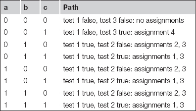
Notice that there are only four distinct cases: no assignment, assignment 4, assignments 2 and 3, or assignments 1 and 3. These correspond to the possible paths through the nested ifs; the table adds value by telling us which variable values exercise each of these paths.
Enumerating the paths through a fixed-iteration for loop is seemingly simple. In the code below,
for (i = 0; i < N; i++)
a[i] = b[i]*c[i];
the assignment in the loop is performed exactly N times. However, we can’t forget the code executed to set up the loop and to test the iteration variable.
Example 5.9 illustrates how to determine the path through a loop.
Example 5.9 Paths in a Loop
Here is the loop code for the FIR filter of Application Example 2.1:
for (i = 0, f = 0; i < N; i++)
f = f + c[i] * x[i];
By examining the CDFG for the code we can more easily determine how many times various statements are executed. Here is the CDFG once again:
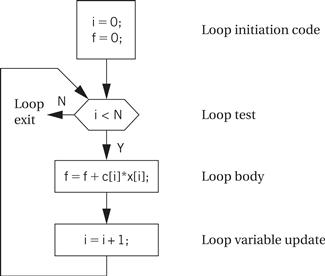
The CDFG makes it clear that the loop initiation block is executed once, the test is executed N + 1 times, and the body and loop variable update are each executed N times.
Instruction timing
Once we know the execution path of the program, we have to measure the execution time of the instructions executed along that path. The simplest estimate is to assume that every instruction takes the same number of clock cycles, which means we need only count the instructions and multiply by the per-instruction execution time to obtain the program’s total execution time. However, even ignoring cache effects, this technique is simplistic for the reasons summarized below.
• Not all instructions take the same amount of time. RISC architectures tend to provide uniform instruction execution times in order to keep the CPU’s pipeline full. But as we saw in Chapter 3, even very simple RISC architectures like the PIC16F take different amounts of time to execute certain instructions. Floating-point instructions show especially wide variations in execution time—while basic multiply and add operations are fast, some transcendental functions can take thousands of cycles to execute.
• Execution times of instructions are not independent. The execution time of one instruction depends on the instructions around it. For example, many CPUs use register bypassing to speed up instruction sequences when the result of one instruction is used in the next instruction. As a result, the execution time of an instruction may depend on whether its destination register is used as a source for the next operation (or vice versa).
• The execution time of an instruction may depend on operand values. This is clearly true of floating-point instructions in which a different number of iterations may be required to calculate the result. Other specialized instructions can, for example, perform a data-dependent number of integer operations.
We can handle the first two problems more easily than the third. We can look up instruction execution time in a table; the table will be indexed by opcode and possibly by other parameter values such as the registers used. To handle interdependent execution times, we can add columns to the table to consider the effects of nearby instructions. Because these effects are generally limited by the size of the CPU pipeline, we know that we need to consider a relatively small window of instructions to handle such effects. Handling variations due to operand values is difficult to do without actually executing the program using a variety of data values, given the large number of factors that can affect value-dependent instruction timing. Luckily, these effects are often small. Even in floating-point programs, most of the operations are typically additions and multiplications whose execution times have small variances.
Caching effects
Thus far we have not considered the effect of the cache. Because the access time for main memory can be 10–100 times larger than the cache access time, caching can have huge effects on instruction execution time by changing both the instruction and data access times. Caching performance inherently depends on the program’s execution path because the cache’s contents depend on the history of accesses.
5.6.2 Measurement-Driven Performance Analysis
The most direct way to determine the execution time of a program is by measuring it. This approach is appealing but it does have some drawbacks. First, in order to cause the program to execute its worst-case execution path, we have to provide the proper inputs to it. Determining the set of inputs that will guarantee the worst-case execution path is infeasible. Furthermore, in order to measure the program’s performance on a particular type of CPU, we need the CPU or its simulator.
Despite these problems, measurement is the most commonly used way to determine the execution time of embedded software. Worst-case execution time analysis algorithms have been used successfully in some areas, such as flight control software, but many system design projects determine the execution time of their programs by measurement.
Program traces
Most methods of measuring program performance combine the determination of the execution path and the timing of that path: as the program executes, it chooses a path and we observe the execution time along that path. We refer to the record of the execution path of a program as a program trace (or more succinctly, a trace). Traces can be valuable for other purposes, such as analyzing the cache behavior of the program.
Measurement issues
Perhaps the biggest problem in measuring program performance is figuring out a useful set of inputs to give the program. This problem has two aspects. First, we have to determine the actual input values. We may be able to use benchmark data sets or data captured from a running system to help us generate typical values. For simple programs, we may be able to analyze the algorithm to determine the inputs that cause the worst-case execution time. The software testing methods of Section 5.10 can help us generate some test values and determine how thoroughly we have exercised the program.
The other problem with input data is the software scaffolding that we may need to feed data into the program and get data out. When we are designing a large system, it may be difficult to extract out part of the software and test it independently of the other parts of the system. We may need to add new testing modules to the system software to help us introduce testing values and to observe testing outputs.
We can measure program performance either directly on the hardware or by using a simulator. Each method has its advantages and disadvantages.
Profiling
Profiling is a simple method for analyzing software performance. A profiler does not measure execution time—instead, it counts the number of times that procedures or basic blocks in the program are executed. There are two major ways to profile a program: we can modify the executable program by adding instructions that increment a location every time the program passes that point in the program; or we can sample the program counter during execution and keep track of the distribution of PC values. Profiling adds relatively little overhead to the program and it gives us some useful information about where the program spends most of its time.
Physical performance measurement
Physical measurement requires some sort of hardware instrumentation. The most direct method of measuring the performance of a program would be to watch the program counter’s value: start a timer when the PC reaches the program’s start, stop the timer when it reaches the program’s end. Unfortunately, it generally isn’t possible to directly observe the program counter. However, it is possible in many cases to modify the program so that it starts a timer at the beginning of execution and stops the timer at the end. While this doesn’t give us direct information about the program trace, it does give us execution time. If we have several timers available, we can use them to measure the execution time of different parts of the program.
A logic analyzer or an oscilloscope can be used to watch for signals that mark various points in the execution of the program. However, because logic analyzers have a limited amount of memory, this approach doesn’t work well for programs with extremely long execution times.
Some CPUs have hardware facilities for automatically generating trace information. For example, the Pentium family microprocessors generate a special bus cycle, a branch trace message, that shows the source and/or destination address of a branch [Col97]. If we record only traces, we can reconstruct the instructions executed within the basic blocks while greatly reducing the amount of memory required to hold the trace.
Hardware traces
The alternative to physical measurement of execution time is simulation. A CPU simulator is a program that takes as input a memory image for a CPU and performs the operations on that memory image that the actual CPU would perform, leaving the results in the modified memory image. For purposes of performance analysis, the most important type of CPU simulator is the cycle-accurate simulator, which performs a sufficiently detailed simulation of the processor’s internals that it can determine the exact number of clock cycles required for execution. A cycle-accurate simulator is built with detailed knowledge of how the processor works, so that it can take into account all the possible behaviors of the microarchitecture that may affect execution time. Cycle-accurate simulators are slower than the processor itself, but a variety of techniques can be used to make them surprisingly fast, running only hundreds of times slower than the hardware itself. A simulator that functionally simulates instructions but does not provide timing information is known as an instruction-level simulator.
Simulation-based performance measurement
A cycle-accurate simulator has a complete model of the processor, including the cache. It can therefore provide valuable information about why the program runs too slowly. The next example discusses a simulator that can be used to model many different processors.
Example 5.10 Cycle-Accurate Simulation
SimpleScalar (http://www.simplescalar.com) is a framework for building cycle-accurate CPU models. Some aspects of the processor can be configured easily at run time. For more complex changes, we can use the SimpleScalar toolkit to write our own simulator.
We can use SimpleScalar to simulate the FIR filter code. SimpleScalar can model a number of different processors; we will use a standard ARM model here.
We want to include the data as part of the program so that the execution time doesn’t include file I/O. File I/O is slow and the time it takes to read or write data can change substantially from one execution to another. We get around this problem by setting up an array that holds the FIR data. And because the test program will include some initialization and other miscellaneous code, we execute the FIR filter many times in a row using a simple loop. Here is the complete test program:
#define COUNT 100
#define N 12
int x[N] = {8,17,3,122,5,93,44,2,201,11,74,75};
int c[N] = {1,2,4,7,3,4,2,2,5,8,5,1};
main() {
int i, k, f;
for (k=0; k<COUNT; k++) { /* run the filter */
for (i=0; i<N; i++)
f += c[i]*x[i];
}
}
To start the simulation process, we compile our test program using a special compiler:
% arm-linux-gcc firtest.c
This gives us an executable program (by default, a.out) that we use to simulate our program:
% arm-outorder a.out
SimpleScalar produces a large output file with a great deal of information about the program’s execution. Because this is a simple example, the most useful piece of data is the total number of simulated clock cycles required to execute the program:
sim_cycle 25854 × total simulation time in cycles
To make sure that we can ignore the effects of program overhead, we will execute the FIR filter for several different values of N and compare. This run used N = 100; when we also run N = 1,000 and N = 10,000, we get these results:
| N | Total simulation time in cycles | Simulation time for one filter execution |
| 100 | 25854 | 259 |
| 1,000 | 155759 | 156 |
| 10,000 | 1451840 | 145 |
Because the FIR filter is so simple and ran in so few cycles, we had to execute it a number of times to wash out all the other overhead of program execution. However, the time for 1,000 and 10,000 filter executions are within 10% of each other, so those values are reasonably close to the actual execution time of the FIR filter itself.
5.7 Software Performance Optimization
In this section we will look at several techniques for optimizing software performance, including both loop and cache optimizations as well as more generic strategies.
5.7.1 Loop Optimizations
Loops are important targets for optimization because programs with loops tend to spend a lot of time executing those loops. There are three important techniques in optimizing loops: code motion, induction variable elimination, and strength reduction.
Code motion lets us move unnecessary code out of a loop. If a computation’s result does not depend on operations performed in the loop body, then we can safely move it out of the loop. Code motion opportunities can arise because programmers may find some computations clearer and more concise when put in the loop body, even though they are not strictly dependent on the loop iterations. A simple example of code motion is also common. Consider this loop:
for (i = 0; i < N*M; i++) {
z[i] = a[i] + b[i];
}
The code motion opportunity becomes more obvious when we draw the loop’s CDFG as shown in Figure 5.22. The loop bound computation is performed on every iteration during the loop test, even though the result never changes. We can avoid N × M − 1 unnecessary executions of this statement by moving it before the loop, as shown in the figure.
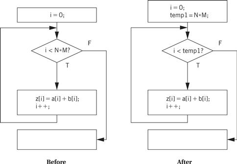
Figure 5.22 Code motion in a loop.
An induction variable is a variable whose value is derived from the loop iteration variable’s value. The compiler often introduces induction variables to help it implement the loop. Properly transformed, we may be able to eliminate some variables and apply strength reduction to others.
A nested loop is a good example of the use of induction variables. Here is a simple nested loop:
for (i = 0; i < N; i++)
for (j = 0; j < M; j++)
z[i][j] = b[i][j];
The compiler uses induction variables to help it address the arrays. Let us rewrite the loop in C using induction variables and pointers. (Later, we use a common induction variable for the two arrays, even though the compiler would probably introduce separate induction variables and then merge them.)
for (i = 0; i < N; i++)
for (j = 0; j < M; j++) {
zbinduct = i*M + j;
*(zptr + zbinduct) = *(bptr + zbinduct);
}
In the above code, zptr and bptr are pointers to the heads of the z and b arrays and zbinduct is the shared induction variable. However, we do not need to compute zbinduct afresh each time. Because we are stepping through the arrays sequentially, we can simply add the update value to the induction variable:
zbinduct = 0;
for (i = 0; i < N; i++) {
for (j = 0; j < M; j++) {
*(zptr + zbinduct) = *(bptr + zbinduct);
zbinduct++;
}
}
This is a form of strength reduction because we have eliminated the multiplication from the induction variable computation.
Strength reduction helps us reduce the cost of a loop iteration. Consider this assignment:
y = x * 2;
In integer arithmetic, we can use a left shift rather than a multiplication by 2 (as long as we properly keep track of overflows). If the shift is faster than the multiply, we probably want to perform the substitution. This optimization can often be used with induction variables because loops are often indexed with simple expressions. Strength reduction can often be performed with simple substitution rules because there are relatively few interactions between the possible substitutions.
5.7.2 Cache Optimizations
A loop nest is a set of loops, one inside the other. Loop nests occur when we process arrays. A large body of techniques has been developed for optimizing loop nests. Rewriting a loop nest changes the order in which array elements are accessed. This can expose new parallelism opportunities that can be exploited by later stages of the compiler, and it can also improve cache performance. In this section we concentrate on the analysis of loop nests for cache performance.
The next example looks at two cache-oriented loop nest optimizations.
Programming Example 5.6 Data Realignment and Array Padding
Assume we want to optimize the cache behavior of the following code:
for (j = 0; j < M; j++)
for (i = 0; i < N; i++)
a[j][i] = b[j][i] * c;
Let us also assume that the a and b arrays are sized with M at 265 and N at 4 and a 256-line, four-way set-associative cache with four words per line. Even though this code does not reuse any data elements, cache conflicts can cause serious performance problems because they interfere with spatial reuse at the cache line level.
Assume that the starting location for a[] is 1024 and the starting location for b[] is 4099. Although a[0][0] and b[0][0] do not map to the same word in the cache, they do map to the same block.
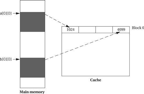
As a result, we see the following scenario in execution:
• The access to a[0][0] brings in the first four words of a[].
• The access to b[0][0] replaces a[0][0] through a[0][3] with b[0][3] and the contents of the three locations before b[].
• When a[0][1] is accessed, the same cache line is again replaced with the first four elements of a[].
Once the a[0][1] access brings that line into the cache, it remains there for the a[0][2] and a[0][3] accesses because the b[] accesses are now on the next line. However, the scenario repeats itself at a[1][0] and every four iterations of the cache.
One way to eliminate the cache conflicts is to move one of the arrays. We do not have to move it far. If we move b’s start to 4100, we eliminate the cache conflicts.
However, that fix won’t work in more complex situations. Moving one array may only introduce cache conflicts with another array. In such cases, we can use another technique called padding. If we extend each of the rows of the arrays to have four elements rather than three, with the padding word placed at the beginning of the row, we eliminate the cache conflicts. In this case, b[0][0] is located at 4100 by the padding. Although padding wastes memory, it substantially improves memory performance. In complex situations with multiple arrays and sophisticated access patterns, we have to use a combination of techniques—relocating arrays and padding them—to be able to minimize cache conflicts.
5.7.3 Performance Optimization Strategies
Let’s look more generally at how to improve program execution time. First, make sure that the code really needs to run faster. Performance analysis and measurement will give you a baseline for the execution time of the program. Knowing the overall execution time tells you how much it needs to be improved. Knowing the execution time of various pieces of the program helps you identify the right locations for changes to the program.
You may be able to redesign your algorithm to improve efficiency. Examining asymptotic performance is often a good guide to efficiency. Doing fewer operations is usually the key to performance. In a few cases, however, brute force may provide a better implementation. A seemingly simple high-level-language statement may in fact hide a very long sequence of operations that slows down the algorithm. Using dynamically allocated memory is one example, because managing the heap takes time but is hidden from the programmer. For example, a sophisticated algorithm that uses dynamic storage may be slower in practice than an algorithm that performs more operations on statically allocated memory.
Finally, you can look at the implementation of the program itself. Here are a few hints on program implementation:
• Try to use registers efficiently. Group accesses to a value together so that the value can be brought into a register and kept there.
• Make use of page mode accesses in the memory system whenever possible. Page mode reads and writes eliminate one step in the memory access. You can increase use of page mode by rearranging your variables so that more can be referenced contiguously.
• Analyze cache behavior to find major cache conflicts. Restructure the code to eliminate as many of these as you can as follows:
• For instruction conflicts, if the offending code segment is small, try to rewrite the segment to make it as small as possible so that it better fits into the cache. Writing in assembly language may be necessary. For conflicts across larger spans of code, try moving the instructions or padding with NOPs.
• For scalar data conflicts, move the data values to different locations to reduce conflicts.
• For array data conflicts, consider either moving the arrays or changing your array access patterns to reduce conflicts.
5.8 Program-Level Energy and Power Analysis and Optimization
Power consumption is a particularly important design metric for battery-powered systems because the battery has a very limited lifetime. However, power consumption is increasingly important in systems that run off the power grid. Fast chips run hot and controlling power consumption is an important element of increasing reliability and reducing system cost.
How much control do we have over power consumption? Ultimately, we must consume the energy required to perform necessary computations. However, there are opportunities for saving power:
• We may be able to replace the algorithms with others that do things in clever ways that consume less power.
• Memory accesses are a major component of power consumption in many applications. By optimizing memory accesses we may be able to significantly reduce power.
• We may be able to turn off parts of the system—such as subsystems of the CPU, chips in the system, and so on—when we don’t need them in order to save power.
The first step in optimizing a program’s energy consumption is knowing how much energy the program consumes. It is possible to measure power consumption for an instruction or a small code fragment [Tiw94]. The technique, illustrated in Figure 5.23, executes the code under test over and over in a loop. By measuring the current flowing into the CPU, we are measuring the power consumption of the complete loop, including both the body and other code. By separately measuring the power consumption of a loop with no body (making sure, of course, that the compiler hasn’t optimized away the empty loop), we can calculate the power consumption of the loop body code as the difference between the full loop and the bare loop energy cost of an instruction.
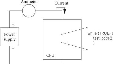
Figure 5.23 Measuring energy consumption for a piece of code.
Several factors contribute to the energy consumption of the program:
• Energy consumption varies somewhat from instruction to instruction.
Choosing which instructions to use can make some difference in a program’s energy consumption, but concentrating on the instruction opcodes has limited payoffs in most CPUs. The program has to do a certain amount of computation to perform its function. While there may be some clever ways to perform that computation, the energy cost of the basic computation will change only a fairly small amount compared to the total system energy consumption, and usually only after a great deal of effort. We are further hampered in our ability to optimize instruction-level energy consumption because most manufacturers do not provide detailed, instruction-level energy consumption figures for their processors.
Memory effects
In many applications, the biggest payoff in energy reduction for a given amount of designer effort comes from concentrating on the memory system. Memory transfers are by far the most expensive type of operation performed by a CPU [Cat98]—a memory transfer requires tens or hundreds of times more energy than does an arithmetic operation. As a result, the biggest payoffs in energy optimization come from properly organizing instructions and data in memory. Accesses to registers are the most energy efficient; cache accesses are more energy efficient than main memory accesses.
Caches are an important factor in energy consumption. On the one hand, a cache hit saves a costly main memory access, and on the other, the cache itself is relatively power hungry because it is built from SRAM, not DRAM. If we can control the size of the cache, we want to choose the smallest cache that provides us with the necessary performance. Li and Henkel [Li98] measured the influence of caches on energy consumption in detail. Figure 5.24 breaks down the energy consumption of a computer running MPEG (a video encoder) into several components: software running on the CPU, main memory, data cache, and instruction cache.
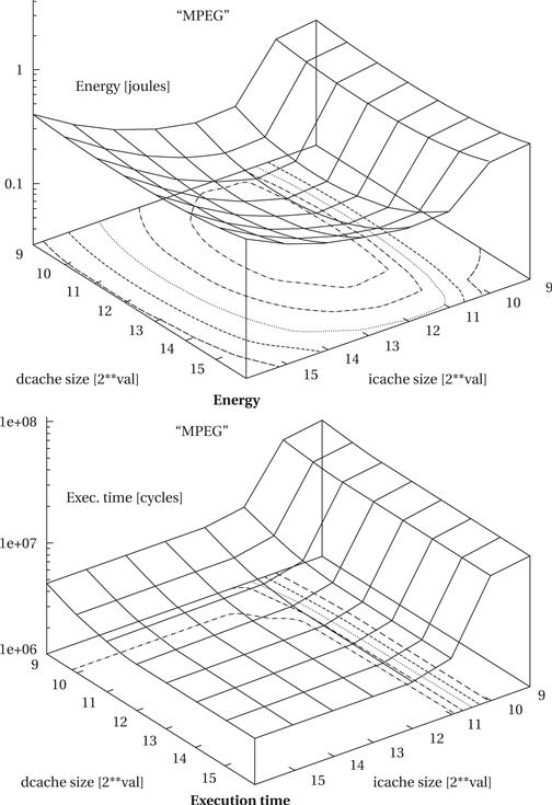
Figure 5.24 Energy and execution time vs. instruction/data cache size for a benchmark program [Li98].
As the instruction cache size increases, the energy cost of the software on the CPU declines, but the instruction cache comes to dominate the energy consumption. Experiments like this on several benchmarks show that many programs have sweet spots in energy consumption. If the cache is too small, the program runs slowly and the system consumes a lot of power due to the high cost of main memory accesses. If the cache is too large, the power consumption is high without a corresponding payoff in performance. At intermediate values, the execution time and power consumption are both good.
Energy optimization
How can we optimize a program for low power consumption? The best overall advice is that high performance = low power. Generally speaking, making the program run faster also reduces energy consumption.
Clearly, the biggest factor that can be reasonably well controlled by the programmer is the memory access patterns. If the program can be modified to reduce instruction or data cache conflicts, for example, the energy required by the memory system can be significantly reduced. The effectiveness of changes such as reordering instructions or selecting different instructions depends on the processor involved, but they are generally less effective than cache optimizations.
A few optimizations mentioned previously for performance are also often useful for improving energy consumption:
• Try to use registers efficiently. Group accesses to a value together so that the value can be brought into a register and kept there.
• Analyze cache behavior to find major cache conflicts. Restructure the code to eliminate as many of these as you can:
• For instruction conflicts, if the offending code segment is small, try to rewrite the segment to make it as small as possible so that it better fits into the cache. Writing in assembly language may be necessary. For conflicts across larger spans of code, try moving the instructions or padding with NOPs.
• For scalar data conflicts, move the data values to different locations to reduce conflicts.
• For array data conflicts, consider either moving the arrays or changing your array access patterns to reduce conflicts.
• Make use of page mode accesses in the memory system whenever possible. Page mode reads and writes eliminate one step in the memory access, saving a considerable amount of power.
Metha et al. [Met97] present some additional observations about energy optimization:
• Moderate loop unrolling eliminates some loop control overhead. However, when the loop is unrolled too much, power increases due to the lower hit rates of straight-line code.
• Software pipelining reduces pipeline stalls, thereby reducing the average energy per instruction.
• Eliminating recursive procedure calls where possible saves power by getting rid of function call overhead. Tail recursion can often be eliminated; some compilers do this automatically.
5.9 Analysis and Optimization of Program Size
The memory footprint of a program is determined by the size of its data and instructions. Both must be considered to minimize program size.
Data provide an excellent opportunity for minimizing size because the data are most highly dependent on programming style. Because inefficient programs often keep several copies of data, identifying and eliminating duplications can lead to significant memory savings usually with little performance penalty. Buffers should be sized carefully—rather than defining a data array to a large size that the program will never attain, determine the actual maximum amount of data held in the buffer and allocate the array accordingly. Data can sometimes be packed, such as by storing several flags in a single word and extracting them by using bit-level operations.
A very low-level technique for minimizing data is to reuse values. For instance, if several constants happen to have the same value, they can be mapped to the same location. Data buffers can often be reused at several different points in the program. This technique must be used with extreme caution, however, because subsequent versions of the program may not use the same values for the constants. A more generally applicable technique is to generate data on the fly rather than store it. Of course, the code required to generate the data takes up space in the program, but when complex data structures are involved there may be some net space savings from using code to generate data.
Minimizing the size of the instruction text of a program requires a mix of high-level program transformations and careful instruction selection. Encapsulating functions in subroutines can reduce program size when done carefully. Because subroutines have overhead for parameter passing that is not obvious from the high-level language code, there is a minimum-size function body for which a subroutine makes sense. Architectures that have variable-size instruction lengths are particularly good candidates for careful coding to minimize program size, which may require assembly language coding of key program segments. There may also be cases in which one or a sequence of instructions is much smaller than alternative implementations—for example, a multiply-accumulate instruction may be both smaller and faster than separate arithmetic operations.
When reducing the number of instructions in a program, one important technique is the proper use of subroutines. If the program performs identical operations repeatedly, these operations are natural candidates for subroutines. Even if the operations vary somewhat, you may be able to construct a properly parameterized subroutine that saves space. Of course, when considering the code size savings, the subroutine linkage code must be counted into the equation. There is extra code not only in the subroutine body but in each call to the subroutine that handles parameters. In some cases, proper instruction selection may reduce code size; this is particularly true in CPUs that use variable-length instructions.
Some microprocessor architectures support dense instruction sets, specially designed instruction sets that use shorter instruction formats to encode the instructions. The ARM Thumb instruction set and the MIPS-16 instruction set for the MIPS architecture are two examples of this type of instruction set. In many cases, a microprocessor that supports the dense instruction set also supports the normal instruction set, although it is possible to build a microprocessor that executes only the dense instruction set. Special compilation modes produce the program in terms of the dense instruction set. Program size of course varies with the type of program, but programs using the dense instruction set are often 70–80% of the size of the standard instruction set equivalents.
5.10 Program Validation and Testing
Complex systems need testing to ensure that they work as they are intended. But bugs can be subtle, particularly in embedded systems, where specialized hardware and real-time responsiveness make programming more challenging. Fortunately, there are many available techniques for software testing that can help us generate a comprehensive set of tests to ensure that our system works properly. We examine the role of validation in the overall design methodology in Section 9.6. In this section, we concentrate on nuts-and-bolts techniques for creating a good set of tests for a given program.
The first question we must ask ourselves is how much testing is enough. Clearly, we cannot test the program for every possible combination of inputs. Because we cannot implement an infinite number of tests, we naturally ask ourselves what a reasonable standard of thoroughness is. One of the major contributions of software testing is to provide us with standards of thoroughness that make sense. Following these standards does not guarantee that we will find all bugs. But by breaking the testing problem into subproblems and analyzing each subproblem, we can identify testing methods that provide reasonable amounts of testing while keeping the testing time within reasonable bounds.
We can use various combinations of two major types of testing strategies:
• Black-box methods generate tests without looking at the internal structure of the program.
• Clear-box (also known as white-box) methods generate tests based on the program structure.
In this section we cover both types of tests, which complement each other by exercising programs in very different ways.
5.10.1 Clear-Box Testing
The control/data flow graph extracted from a program’s source code is an important tool in developing clear-box tests for the program. To adequately test the program, we must exercise both its control and data operations.
In order to execute and evaluate these tests, we must be able to control variables in the program and observe the results of computations, much as in manufacturing testing. In general, we may need to modify the program to make it more testable. By adding new inputs and outputs, we can usually substantially reduce the effort required to find and execute the test. No matter what we are testing, we must accomplish the following three things in a test:
• Provide the program with inputs that exercise the test we are interested in.
• Execute the program to perform the test.
• Examine the outputs to determine whether the test was successful.
Example 5.11 illustrates the importance of observability and controllability in software testing.
Example 5.11 Controlling and Observing Programs
Let’s first consider controllability by examining the following FIR filter with a limiter:
firout = 0.0; /* initialize filter output */
/* compute buff*c in bottom part of circular buffer */
for (j = curr, k = 0; j < N; j++, k++)
firout += buff[j] * c[k];
/* compute buff*c in top part of circular buffer */
for (j = 0; j < curr; j++, k++)
firout += buff[j] * c[k];
/* limit output value */
if (firout > 100.0) firout = 100.0;
if (firout < −100.0) firout = −100.0;
The above code computes the output of an FIR filter from a circular buffer of values and then limits the maximum filter output (much as an overloaded speaker will hit a range limit). If we want to test whether the limiting code works, we must be able to generate two out-of-range values for firout: positive and negative. To do that, we must fill the FIR filter’s circular buffer with N values in the proper range. Although there are many sets of values that will work, it will still take time for us to properly set up the filter output for each test.
This code also illustrates an observability problem. If we want to test the FIR filter itself, we look at the value of firout before the limiting code executes. We could use a debugger to set breakpoints in the code, but this is an awkward way to perform a large number of tests. If we want to test the FIR code independent of the limiting code, we would have to add a mechanism for observing firout independently.
Being able to perform this process for a large number of tests entails some amount of drudgery, but that drudgery can be alleviated with good program design that simplifies controllability and observability.
The next task is to determine the set of tests to be performed. We need to perform many different types of tests to be confident that we have identified a large fraction of the existing bugs. Even if we thoroughly test the program using one criterion, that criterion ignores other aspects of the program. Over the next few pages we will describe several very different criteria for program testing.
Execution paths
The most fundamental concept in clear-box testing is the path of execution through a program. Previously, we considered paths for performance analysis; we are now concerned with making sure that a path is covered and determining how to ensure that the path is in fact executed. We want to test the program by forcing the program to execute along chosen paths. We force the execution of a path by giving it inputs that cause it to take the appropriate branches. Execution of a path exercises both the control and data aspects of the program. The control is exercised as we take branches; both the computations leading up to the branch decision and other computations performed along the path exercise the data aspects.
Is it possible to execute every complete path in an arbitrary program? The answer is no, because the program may contain a while loop that is not guaranteed to terminate. The same is true for any program that operates on a continuous stream of data, because we cannot arbitrarily define the beginning and end of the data stream. If the program always terminates, then there are indeed a finite number of complete paths that can be enumerated from the path graph. This leads us to the next question: Does it make sense to exercise every path? The answer to this question is no for most programs, because the number of paths, especially for any program with a loop, is extremely large. However, the choice of an appropriate subset of paths to test requires some thought.
Example 5.12 illustrates the consequences of two different choices of testing strategies.
Example 5.12 Choosing the Paths to Test
We have at least two reasonable ways to choose a set of paths in a program to test:
These conditions are equivalent for structured programming languages without gotos, but are not the same for unstructured code. Most assembly language is unstructured, and state machines may be coded in high-level languages with gotos.
To understand the difference between statement and branch coverage, consider this CDFG:
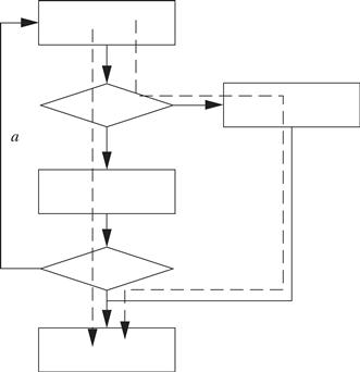
We can execute every statement at least once by executing the program along two distinct paths. However, this leaves branch a out of the lower conditional uncovered. To ensure that we have executed along every edge in the CDFG, we must execute a third path through the program. This path does not test any new statements, but it does cause a to be exercised.
How do we choose a set of paths that adequately covers the program’s behavior? Intuition tells us that a relatively small number of paths should be able to cover most practical programs. Graph theory helps us get a quantitative handle on the different paths required. In an undirected graph, we can form any path through the graph from combinations of basis paths. (Unfortunately, this property does not strictly hold for directed graphs such as CDFGs, but this formulation still helps us understand the nature of selecting a set of covering paths through a program.) The term “basis set” comes from linear algebra. Figure 5.25 shows how to evaluate the basis set of a graph. The graph is represented as an incidence matrix. Each row and column represents a node; a 1 is entered for each node pair connected by an edge. We can use standard linear algebra techniques to identify the basis set of the graph. Each vector in the basis set represents a primitive path. We can form new paths by adding the vectors modulo 2. Generally, there is more than one basis set for a graph.
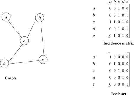
Figure 5.25 The matrix representation of a graph and its basis set.
The basis set property provides a metric for test coverage. If we cover all the basis paths, we can consider the control flow adequately covered. Although the basis set measure is not entirely accurate because the directed edges of the CDFG may make some combinations of paths infeasible, it does provide a reasonable and justifiable measure of test coverage.
A simple measure, cyclomatic complexity[McC76], allows us to measure the control complexity of a program. Cyclomatic complexity is an upper bound on the size of the basis set. If e is the number of edges in the flow graph, n the number of nodes, and p the number of components in the graph, then the cyclomatic complexity is given by
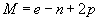 (Eq. 5.1)
For a structured program, M can be computed by counting the number of binary decisions in the flow graph and adding 1. If the CDFG has higher-order branch nodes, add b − 1 for each b-way branch. In the example of Figure 5.26, the cyclomatic complexity evaluates to 4. Because there are actually only three distinct paths in the graph, cyclomatic complexity in this case is an overly conservative bound.
Figure 5.26 Cyclomatic complexity.
Another way of looking at control flow–oriented testing is to analyze the conditions that control the conditional statements. Consider the following if statement:
if ((a == b) || (c >= d)) { … }
This complex condition can be exercised in several different ways. If we want to truly exercise the paths through this condition, it is prudent to exercise the conditional’s elements in ways related to their own structure, not just the structure of the paths through them. A simple condition testing strategy is known as branch testing[Mye79]. This strategy requires the true and false branches of a conditional and every simple condition in the conditional’s expression to be tested at least once.
Example 5.13 illustrates branch testing.
Example 5.13 Condition Testing with the Branch Testing Strategy
Assume that the code below is what we meant to write.
if (a || (b >= c)) { printf("OK\n"); }
The code that we mistakenly wrote instead follows:
if (a && (b >= c)) { printf("OK\n"); }
If we apply branch testing to the code we wrote, one of the tests will use these values: a = 0, b = 3, c = 2 (making a false and b >= c true). In this case, the code should print the OK term [0 || (3 >= 2) is true] but instead doesn’t print [0 && (3 >= 2) evaluates to false]. That test picks up the error.
Let’s consider another more subtle error that is nonetheless all too common in C. The code we meant to write follows:
if ((x == good_pointer) && (x->field1 == 3)) { printf("got the value\n"); }
Here is the bad code we actually wrote:
if ((x = good_pointer) && (x->field1 == 3)) { printf("got the value\n"); }
The problem here is that we typed = rather than ==, creating an assignment rather than a test. The code x = good_pointer first assigns the value good_pointer to x and then, because assignments are also expressions in C, returns good_pointer as the result of evaluating this expression.
If we apply the principles of branch testing, one of the tests we want to use will contain x != good_pointer and x->field1 == 3. Whether this test catches the error depends on the state of the record pointed to by good_pointer. If it is equal to 3 at the time of the test, the message will be printed erroneously. Although this test is not guaranteed to uncover the bug, it has a reasonable chance of success. One of the reasons to use many different types of tests is to maximize the chance that supposedly unrelated elements will cooperate to reveal the error in a particular situation.
Another more sophisticated strategy for testing conditionals is known as domain testing [How82], illustrated in Figure 5.27. Domain testing concentrates on linear inequalities. In the figure, the inequality the program should use for the test is j < = i + 1. We test the inequality with three test points—two on the boundary of the valid region and a third outside the region but between the i values of the other two points. When we make some common mistakes in typing the inequality, these three tests are sufficient to uncover them, as shown in the figure.
Figure 5.27 Domain testing for a pair of values.
A potential problem with path coverage is that the paths chosen to cover the CDFG may not have any important relationship to the program’s function. Another testing strategy known as data flow testing makes use of def-use analysis (short for definition-use analysis). It selects paths that have some relationship to the program’s function.
The terms def and use come from compilers, which use def-use analysis for optimization [Aho06]. A variable’s value is defined when an assignment is made to the variable; it is used when it appears on the right side of an assignment (sometimes called a C-use for computation use) or in a conditional expression (sometimes called P-use for predicate use). A def-use pair is a definition of a variable’s value and a use of that value. Figure 5.28 shows a code fragment and all the def-use pairs for the first assignment to a. Def-use analysis can be performed on a program using iterative algorithms. Data flow testing chooses tests that exercise chosen def-use pairs. The test first causes a certain value to be assigned at the definition and then observes the result at the use point to be sure that the desired value arrived there. Frankl and Weyuker [Fra88] have defined criteria for choosing which def-use pairs to exercise to satisfy a well-behaved adequacy criterion.
Figure 5.28 Definitions and uses of variables.
Testing loops
We can write some specialized tests for loops. Because loops are common and often perform important steps in the program, it is worth developing loop-centric testing methods. If the number of iterations is fixed, then testing is relatively simple. However, many loops have bounds that are executed at run time.
Consider first the case of a single loop:
for (i = 0; i < terminate(); i++)
proc(i,array);
It would be too expensive to evaluate the above loop for all possible termination conditions. However, there are several important cases that we should try at a minimum:
1. Skipping the loop entirely [if possible, such as when terminate() returns 0 on its first call].
4. If there is an upper bound n on the number of loop iterations (which may come from the maximum size of an array), a value that is significantly below that maximum number of iterations.
5. Tests near the upper bound on the number of loop iterations, that is, n − 1, n, and n + 1.
We can also have nested loops like this:
for (i = 0; i < terminate1(); i++)
for (j = 0; j < terminate2(); j++)
for (k = 0; k < terminate3(); k++)
proc(i,j,k,array);
There are many possible strategies for testing nested loops. One thing to keep in mind is which loops have fixed versus variable numbers of iterations. Beizer [Bei90] suggests an inside-out strategy for testing loops with multiple variable iteration bounds. First, concentrate on testing the innermost loop as above—the outer loops should be controlled to their minimum numbers of iterations. After the inner loop has been thoroughly tested, the next outer loop can be tested more thoroughly, with the inner loop executing a typical number of iterations. This strategy can be repeated until the entire loop nest has been tested. Clearly, nested loops can require a large number of tests. It may be worthwhile to insert testing code to allow greater control over the loop nest for testing.
5.10.2 Black-Box Testing
Black-box tests are generated without knowledge of the code being tested. When used alone, black-box tests have a low probability of finding all the bugs in a program. But when used in conjunction with clear-box tests they help provide a well-rounded test set, because black-box tests are likely to uncover errors that are unlikely to be found by tests extracted from the code structure. Black-box tests can really work. For instance, when asked to test an instrument whose front panel was run by a microcontroller, one acquaintance of the author used his hand to depress all the buttons simultaneously. The front panel immediately locked up. This situation could occur in practice if the instrument were placed face-down on a table, but discovery of this bug would be very unlikely via clear-box tests.
One important technique is to take tests directly from the specification for the code under design. The specification should state which outputs are expected for certain inputs. Tests should be created that provide specified outputs and evaluate whether the results also satisfy the inputs.
We can’t test every possible input combination, but some rules of thumb help us select reasonable sets of inputs. When an input can range across a set of values, it is a very good idea to test at the ends of the range. For example, if an input must be between 1 and 10, 0, 1, 10, and 11 are all important values to test. We should be sure to consider tests both within and outside the range, such as, testing values within the range and outside the range. We may want to consider tests well outside the valid range as well as boundary-condition tests.
Random tests
Random tests form one category of black-box test. Random values are generated with a given distribution. The expected values are computed independently of the system, and then the test inputs are applied. A large number of tests must be applied for the results to be statistically significant, but the tests are easy to generate.
Another scenario is to test certain types of data values. For example, integer-valued inputs can be generated at interesting values such as 0, 1, and values near the maximum end of the data range. Illegal values can be tested as well.
Regression tests
Regression tests form an extremely important category of tests. When tests are created during earlier stages in the system design or for previous versions of the system, those tests should be saved to apply to the later versions of the system. Clearly, unless the system specification changed, the new system should be able to pass old tests. In some cases old bugs can creep back into systems, such as when an old version of a software module is inadvertently installed. In other cases regression tests simply exercise the code in different ways than would be done for the current version of the code and therefore possibly exercise different bugs.
Numerical accuracy
Some embedded systems, particularly digital signal processing systems, lend themselves to numerical analysis. Signal processing algorithms are frequently implemented with limited-range arithmetic to save hardware costs. Aggressive data sets can be generated to stress the numerical accuracy of the system. These tests can often be generated from the original formulas without reference to the source code.
5.10.3 Evaluating Functional Tests
How much testing is enough? Horgan and Mathur [Hor96] evaluated the coverage of two well-known programs, TeX and awk. They used functional tests for these programs that had been developed over several years of extensive testing. Upon applying those functional tests to the programs, they obtained the code coverage statistics shown in Figure 5.29. The columns refer to various types of test coverage: block refers to basic blocks, decision to conditionals, P-use to a use of a variable in a predicate (decision), and C-use to variable use in a nonpredicate computation. These results are at least suggestive that functional testing does not fully exercise the code and that techniques that explicitly generate tests for various pieces of code are necessary to obtain adequate levels of code coverage.
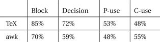
Figure 5.29 Code coverage of functional tests for TeX and awk (after Horgan and Mathur [Hor96]).
Methodological techniques are important for understanding the quality of your tests. For example, if you keep track of the number of bugs tested each day, the data you collect over time should show you some trends on the number of errors per page of code to expect on the average, how many bugs are caught by certain kinds of tests, and so on. We address methodological approaches to quality control in more detail in Chapter 7.
One interesting method for analyzing the coverage of your tests is error injection. First, take your existing code and add bugs to it, keeping track of where the bugs were added. Then run your existing tests on the modified program. By counting the number of added bugs your tests found, you can get an idea of how effective the tests are in uncovering the bugs you haven’t yet found. This method assumes that you can deliberately inject bugs that are of similar varieties to those created naturally by programming errors. If the bugs are too easy or too difficult to find or simply require different types of tests, then bug injection’s results will not be relevant. Of course, it is essential that you finally use the correct code, not the code with added bugs.
5.11 Design Example: Software Modem
In this section we design a modem. Low-cost modems generally use specialized chips, but some PCs implement the modem functions in software. Before jumping into the modem design itself, we discuss principles of how to transmit digital data over a telephone line. We will then go through a specification and discuss architecture, module design, and testing.
5.11.1 Theory of Operation and Requirements
The modem will use frequency-shift keying (FSK), a technique used in 1,200-baud modems. Keying alludes to Morse code–style keying. As shown in Figure 5.30, the FSK scheme transmits sinusoidal tones, with 0 and 1 assigned to different frequencies. Sinusoidal tones are much better suited to transmission over analog phone lines than are the traditional high and low voltages of digital circuits. The 01 bit patterns create the chirping sound characteristic of modems. (Higher-speed modems are backward compatible with the 1,200-baud FSK scheme and begin a transmission with a protocol to determine which speed and protocol should be used.)
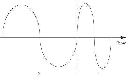
Figure 5.30 Frequency-shift keying.
The scheme used to translate the audio input into a bit stream is illustrated in Figure 5.31. The analog input is sampled and the resulting stream is sent to two digital filters (such as an FIR filter). One filter passes frequencies in the range that represents a 0 and rejects the 1-band frequencies, and the other filter does the converse. The outputs of the filters are sent to detectors, which compute the average value of the signal over the past n samples. When the energy goes above a threshold value, the appropriate bit is detected.
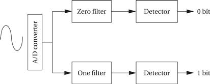
Figure 5.31 The FSK detection scheme.
We will send data in units of 8-bit bytes. The transmitting and receiving modems agree in advance on the length of time during which a bit will be transmitted (otherwise known as the baud rate). But the transmitter and receiver are physically separated and therefore are not synchronized in any way. The receiving modem does not know when the transmitter has started to send a byte. Furthermore, even when the receiver does detect a transmission, the clock rates of the transmitter and receiver may vary somewhat, causing them to fall out of sync. In both cases, we can reduce the chances for error by sending the waveforms for a longer time.
The receiving process is illustrated in Figure 5.32. The receiver will detect the start of a byte by looking for a start bit, which is always 0. By measuring the length of the start bit, the receiver knows where to look for the start of the first bit. However, because the receiver may have slightly misjudged the start of the bit, it does not immediately try to detect the bit. Instead, it runs the detection algorithm at the predicted middle of the bit.
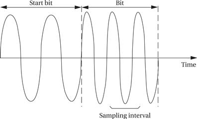
Figure 5.32 Receiving bits in the modem.
The modem will not implement a hardware interface to a telephone line or software for dialing a phone number. We will assume that we have analog audio inputs and outputs for sending and receiving. We will also run at a much slower bit rate than 1,200 baud to simplify the implementation. Next, we will not implement a serial interface to a host, but rather put the transmitter’s message in memory and save the receiver’s result in memory as well. Given those understandings, let’s fill out the requirements table.
| Name | Modem |
| Purpose | A fixed baud rate frequency-shift keyed modem. |
| Inputs | Analog sound input, reset button. |
| Outputs | Analog sound output, LED bit display. |
| Functions | Transmitter: Sends data stored in microprocessor memory in 8-bit bytes. Sends start bit for each byte equal in length to one bit. |
| Receiver: Automatically detects bytes and stores results in main memory. Displays currently received bit on LED. | |
| Performance | 1,200 baud. |
| Manufacturing cost | Dominated by microprocessor and analog I/O. |
| Power | Powered by AC through a standard power supply. |
| Physical size and weight | Small and light enough to fit on a desktop. |
5.11.2 Specification
The basic classes for the modem are shown in Figure 5.33. The classes include physical classes for line-in and line-out plus classes for the receiver and transmitter.
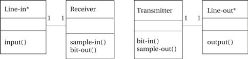
Figure 5.33 Class diagram for the modem.
5.11.3 System Architecture
The modem consists of one small subsystem (the interrupt handlers for the samples) and two major subsystems (transmitter and receiver). Two sample interrupt handlers are required, one for input and another for output, but they are very simple. The transmitter is simpler, so let’s consider its software architecture first.
The best way to generate waveforms that retain the proper shape over long intervals is table lookup. Software oscillators can be used to generate periodic signals, but numerical problems limit their accuracy. Figure 5.34 shows an analog waveform with sample points and the C code for these samples. Table lookup can be combined with interpolation to generate high-resolution waveforms without excessive memory costs, which is more accurate than oscillators because no feedback is involved. The required number of samples for the modem can be found by experimentation with the analog/digital converter and the sampling code.
Figure 5.34 Waveform generation by table lookup.
The structure of the receiver is considerably more complex. The filters and detectors of Figure 5.32 can be implemented with circular buffers. But that module must feed a state machine that recognizes the bits. The recognizer state machine must use a timer to determine when to start and stop computing the filter output average based on the starting point of the bit. It must then determine the nature of the bit at the proper interval. It must also detect the start bit and measure it using the counter. The receiver sample interrupt handler is a natural candidate to double as the receiver timer because the receiver’s time points are relative to samples.
The hardware architecture is relatively simple. In addition to the analog/digital and digital/analog converters, a timer is required. The amount of memory required to implement the algorithms is relatively small.
5.11.4 Component Design and Testing
The transmitter and receiver can be tested relatively thoroughly on the host platform because the timing-critical code only delivers data samples. The transmitter’s output is relatively easy to verify, particularly if the data are plotted. A testbench can be constructed to feed the receiver code sinusoidal inputs and test its bit recognition rate. It is a good idea to test the bit detectors first before testing the complete receiver operation. One potential problem in host-based testing of the receiver is encountered when library code is used for the receiver function. If a DSP library for the target processor is used to implement the filters, then a substitute must be found or built for the host processor testing. The receiver must then be retested when moved to the target system to ensure that it still functions properly with the library code.
Care must be taken to ensure that the receiver does not run too long and miss its deadline. Because the bulk of the computation is in the filters, it is relatively simple to estimate the total computation time early in the implementation process.
5.11.5 System Integration and Testing
There are two ways to test the modem system: by having the modem’s transmitter send bits to its receiver, and or by connecting two different modems. The ultimate test is to connect two different modems, particularly modems designed by different people to be sure that incompatible assumptions or errors were not made. But single-unit testing, called loop-back testing in the telecommunications industry, is simpler and a good first step. Loop-back can be performed in two ways. First, a shared variable can be used to directly pass data from the transmitter to the receiver. Second, an audio cable can be used to plug the analog output to the analog input. In this case it is also possible to inject analog noise to test the resiliency of the detection algorithm.
5.12 Design Example: Digital Still Camera
In this section we design a simple digital still camera (DSC). Video cameras share some similarities with DSCs but are different in several ways, most notably their emphasis on streaming media. We will study a design example for one subsystem of a video camera in Chapter 8.
5.12.1 Theory of Operation and Requirements
In order to understand the digital still camera, we must first understand the digital photography process. A modern digital camera performs a great many steps:
In addition to actually taking the photo, the camera must perform several other important operations, often simultaneously with the picture-taking process. It must, for example, update the camera’s electronic display. It must also listen for button presses from the user, which may command operations that modify the current operation of the camera. The camera should also provide a browser with which the user can review the stored images.
Imaging terminology
Much of this terminology comes largely from film photography—for example, the decisions made while developing a digital photo are similar to those made in the development of a film image, even though the steps to carry out those decisions are very different. Many variations are possible on all of these steps but the basic process is common to all digital still cameras. A few basic terms are useful: the image is divided into pixels; a pixel’s brightness is often referred to as its luminance; a color pixel’s brightness in a particular color is known as chrominance.
Imaging algorithms
The camera can use the image sensor data to drive the exposure-setting process. Several algorithms are possible but all involve starting with a test exposure and using some search algorithm to select the final exposure. Exposure-setting may also use any of several different metrics to judge the exposure. The simplest metric is the average luminance of a pixel. The camera may evaluate some function of several points in the image. It may also evaluate the image’s histogram. The histogram is composed by sorting the pixels into bins by luminance; 256 bins is a common choice for the resolution of the histogram. The histogram gives us more information than does a single average. For instance, we can tell whether many pixels are overexposed or underexposed by looking at the bins at the extremes of luminance.
Three major approaches are used to determine focus: active rangefinding, phase detection, contrast detection. Active rangefinding uses a pulse that is sent out and the time-of-flight of the reflected and returned pulse is measured to determine distance. Ultrasound was used in one early autofocus system, the Polaroid SX-70, but today infrared pulses are more commonly used. Phase detection compares light from opposite sides of the lens, creating an optical rangefinder. Contrast detection relies on the fact that out-of-focused edges do not display the sharp changes in luminance of in-focus edges. The simplest algorithms for contrast detection evaluate focus at pre-determined points in the image, which may require the photographer to move the camera to place a suitable edge at one of the autofocus spots.
Two major types of image sensors are used in modern cameras [Nak05]: charged-coupled devices (CCDs) and CMOS. For our purposes, the operation of these two in a digital still camera are equivalent.
Developing the image involves both putting the image in usable form and improving its quality. The most basic operation required for a color image is to interpolate a full color value for each pixel. Most image sensors capture color images using a color filter array—color filters that cover a single pixel. The filters usually capture one of the primary colors—red, green, and blue—and are arranged in a two-dimensional pattern. The first such color filter array was proposed by Bayer [Bay76]. His pattern is still widely used and known as the Bayer pattern. As shown in Figure 5.35, the Bayer pattern is a 2 × 2 array with two green, one blue, and one red pixels. More green pixels are used because the eye is most sensitive to green, which Bayer viewed as a simple luminance signal. Because each image sensor pixel captured only one of the primaries, the other two primaries must be interpolated for each pixel. This process is known as Bayer pattern interpolation or demosaicing. The simplest interpolation algorithm is a simple average, which can also be used as a low-pass filter. For example, we can interpolate the missing values from the green pixel G2.1 as:
Figure 5.35 A color filter array arranged in a Bayer pattern.
We can use more information to interpolate missing green values. For example, the green value associated with red pixel R1.1 can be interpolated from the four nearest green pixels:

However, this simple interpolation algorithm introduces color fringes at edges. More sophisticated interpolation algorithms exist to minimize color fringing while maintaining other aspects of image quality.
Development also determines and corrects for color temperature in the scene. Different light sources can be composed of light of different colors; color can be described as the temperature of a black body that will emit radiation of that frequency. The human visual system automatically corrects for color temperature. We do not, for example, notice that fluorescent lights emit a greenish cast. However, a photo taken without color temperature correction will display a cast from the color of light used to illuminate the scene. A variety of algorithms exist to determine the color temperature. A set of chrominance histograms is often used to judge color temperature. Once a color correction is determined, it can be applied to the pixels in the image.
Many cameras also apply sharpening algorithms to reduce some of the effects of pixellation in digital image capture. Once again, a variety of sharpening algorithms are used. These algorithms apply filters to sets of adjacent pixels.
Some cameras offer a RAW mode of image capture. The resulting RAW file holds the pixel values without processing. RAW capture allows the user to develop the image manually and offline using sophisticated algorithms and programs. Although generic RAW file formats exist, most camera manufacturers use proprietary RAW formats. Some uncompressed image formats also exist, such as TIFF [Ado92].
Image compression
Compression reduces the amount of storage required for the image. Some lossless compression methods are used that do not throw away information from the image. However, most images are stored using lossy compression. A lossy compression algorithm throws away information in the image, so that the decompression process cannot reproduce an exact copy of the original image. A number of compression techniques have been developed to substantially reduce the storage space required for an image without noticeably affecting image quality. The most common family of compression algorithms is JPEG[CCI92]. (JPEG stands for Joint Photographic Experts Group.) The JPEG standard was extended as JPEG 2000 but classic JPEG is still widely used. The JPEG standard itself contains a large number of options, not all of which need to be implemented to conform to the standard.
As shown in Figure 5.36, the typical compression process used for JPEG images has five main steps:
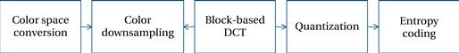
Figure 5.36 The typical JPEG compression process.
(We call this typical because the standard allows for several variations.) The first step puts the color image into a form that allows optimizations less likely to reduce image quality. Color can be represented by a number of color spaces or combinations of colors that, when combined, form the full range of colors. We saw the red/green/blue (RGB) color space in the color filter array. For compression, we convert to the Y’CRCB color space: Y’ is a luminance channel, CR is a red channel, and CB is a blue channel. The conversion between these two color spaces is defined by the JFIF standard [Ham92]:
Once in Y’CRCB form, the CR and CB is generally reduced by downsampling. The 4:2:2 method downsamples both CR and CB to half their normal resolution only in the horizontal direction. The 4:2:0 method downsamples both CR and CB both horizontally and vertically. Downsampling reduces the amount of data required and is justified by the human visual system’s lower acuity in chrominance. The three color channels, Y’, CR , and CB , are processed separately.
The color channels are next separately broken into 8 × 8 blocks (the term block specifically refers to an 8 × 8 array of values in JPEG). The discrete cosine transform is applied to each block. DCT is a frequency transform that produces an 8 × 8 block of transform coefficients. It is reversible, so that the original values can be reconstructed from the transform coefficients. DCT does not itself reduce the amount of information in a block. Many highly optimized algorithms exist to compute the DCT, and in particular an 8 × 8 DCT.
The lossiness of the compression process occurs in the quantization step. This step changes the DCT coefficients with the aim to do so in a way that allows them to be stored in fewer bits. Quantization is applied on the DCT rather than on the pixels because some image characteristics are easier to identify in the DCT representation. Specifically, because the DCT breaks up the block according to spatial frequencies, quantization often reduces the high frequency content of the block. This strategy tends to significantly reduce the data set size during compression while causing less noticeable visual artifacts.
The quantization is defined by an 8 × 8 quantization matrix Q. A DCT coefficient Gi,j is quantized to a value Bi,j using the Qi,j value from the quantization matrix:
The JPEG standard allows for different quantization matrices but gives a typical matrix that is widely used:
This matrix tends to zeroes in the lower-right coefficients. Higher spatial frequencies (and therefore finer detail) are represented by the coefficients in the lower and right parts of the matrix. Putting these to zero eliminates some fine detail from the block.
Quantization does not directly provide for a smaller representation of the image. Entropy coding (lossless encoding) recodes the quantized blocks in a form that requires fewer bits. JPEG allows multiple entropy coding algorithms to be used. The most common algorithm is Huffman coding. The encoding can be represented as a table that maps a fixed number of bits into a variable number of bits. This step encodes the difference between the current coefficient and the previous coefficient, not the coefficient itself. Several different styles of encoding are possible: baseline sequential codes one block at a time; baseline progressive encodes corresponding coefficients of every block.
Coefficients are read from the coefficient matrix in the zig-zag pattern shown in Figure 5.37. This pattern reads along diagonals from the upper left to the lower right, which corresponds to reading from lowest spatial frequency to highest spatial frequency. If fine detail is reduced equally in both horizontal and vertical dimensions, then zero coefficients are also arranged diagonally. The zig-zag pattern increases the length of sequences of zero coefficients in such cases. Long strings of zeroes can be coded in a very small number of bits.
Figure 5.37 Zig-zag pattern for reading coefficients.
The requirements for the digital still camera are given in Figure 5.38.
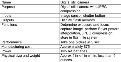
Figure 5.38 Requirements for the digital still camera.
5.12.2 Specification
A digital still camera must comply with a number of standards. These standards generally govern the format of output generated by the camera. Standards in general allow for some freedom of implementation in certain aspects while still adhering to the standard.
File formats
The Tagged Image File Format (TIFF) [Ado92] is often used to store uncompressed images, although it also supports several compression methods as well. Baseline TIFF specifies a basic format that also provides flexibility on image size, bits per pixel, compression, and other aspects of image storage.
The JPEG standard itself allows a number of options that can be followed in various combinations. A set of operations used to generate a compressed image is known as a process. The JFIF standard [Ham92] is a widely used file interchange format. It is compatible with the JPEG standard but specifies a number of items in more detail.
The Exchangeable Image File Format (EXIF) standard is widely used to further extend the information stored in an image file. As shown in Figure 5.39, an EXIF file holds several types of data:
• The metadata section provides a wide range of information: date, time, location, and so on. The metadata is defined as attribute/value pairs. An EXIF file need not contain all possible attributes.
• A thumbnail is a smaller version of a file used for quick display. Thumbnails are widely used both by cameras to display the image on a small screen and on desktop computers to more quickly display a sample of the image. Storage of the thumbnail avoids the need to regenerate the thumbnail each time, saving both computation time and energy.
• JPEG compression data includes tables, such as entropy coding and quantization tables, used to encode the image.
• The compressed JPEG image itself takes up the bulk of the space in the file.
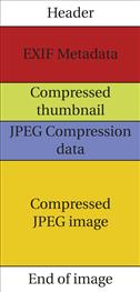
Figure 5.39 Structure of an EXIF file.
The entire image storage process is defined by yet another standard, the Design rule for Camera File (DCF) standard [CIP10]. DCF specifies three major steps: JPEG compression, EXIF file generation, and DOS FAT image storage. DCF specifies a number of aspects of file storage:
• The DCF image root directory is kept in the root directory and is named DCIM (for “digital camera images”).
• The directories within DCIM have names of eight characters, the first three of which are numbers between 100 and 999, giving the directory number. The remaining five characters are required to be upper-case alphanumeric.
• File names in DCF are eight characters long. The first four characters are uppercase alphanumeric, followed by a four digit number between 0001 and 9999.
• Basic files in DCF are in EXIF version 2 format. The standard specifies a number of properties of these EXIF files.
The Digital Print Order Format (DPOF) standard [DPO00] provides a standard way for camera users to order prints of selected photographs. Print orders can be captured in the camera, a home computer, or other devices and transmitted to a photofinisher or printer.
Camera operating modes
Even a simple point-and-shoot camera provides a number of options and modes. Two basic operations are fundamental: display a live view of the current image and capture an image.
Figure 5.40 shows a state diagram for the display. In normal operation, the camera repeatedly displays the latest image from the image sensor. After an image is captured, it is briefly shown on the display.
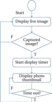
Figure 5.40 State diagram for display operation.
Figure 5.41 shows a state diagram for the picture-taking process. Depressing the shutter button half-way signals the camera to evaluate exposure and focus. Once the shutter is fully depressed, the image is captured, developed, compressed, and stored.
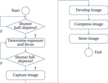
Figure 5.41 State diagram for picture taking.
5.12.3 System Architecture
The basic architecture of a digital still camera uses a controller to provide the basic sequencing for picture taking and camera operation. The controller calls on a number of other units to perform the various steps in each process.
Figure 5.42 shows the basic classes in a digital still camera. The controller class implements the state diagrams for camera operation. The buttons and display classes provide an abstraction of the physical user interface. The image sensor abstracts the operation of the sensor. The picture developer provides algorithms for mosaicing, sharpening, etc. The compression unit generates compressed image data. The file generator takes care of aspects of the file generation beyond compression. The file system performs basic file functions. Cameras may also provide other communication ports such as USB or Firewire.
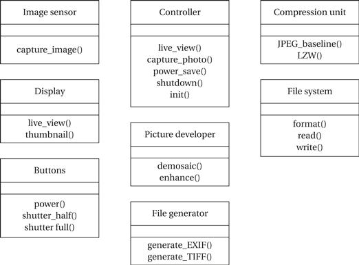
Figure 5.42 Basic classes in the digital still camera.
Figure 5.43 shows a typical block diagram for digital still camera hardware. While some cameras will use the same processor for both system control and image processing, many cameras rely on separate processors for these two tasks. The DSP may be programmable or custom hardware.
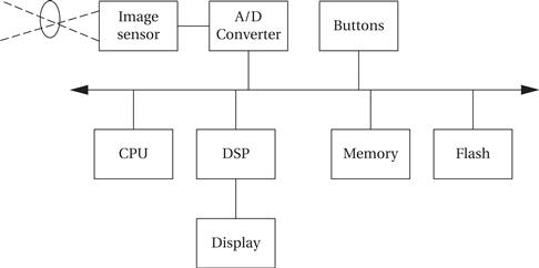
Figure 5.43 Computing platform for a digital still camera.
A sequence diagram for taking a photo is shown in Figure 5.44. This sequence diagram maps the basic operations onto the units in the hardware architecture.
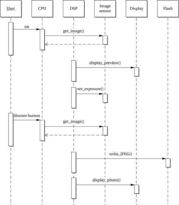
Figure 5.44 Sequence diagram for taking a picture with a digital still camera.
The design of buffering is very important in a digital still camera. Buffering affects the rate at which pictures can be taken, the energy consumed, and the cost of the camera. The image exists in several versions at different points in the process: the raw image from the image sensor; the developed image; the compressed image data; and the file. Most of this data is buffered in system RAM. However, displays may have their own memory to ensure adequate performance.
5.12.4 Component Design and Testing
Components based on standards, such as JPEG or FAT, may be implemented using modules developed elsewhere. JPEG compression in particular may be implemented with special-purpose hardware. DCT accelerators are common. Some digital still camera engines use hardware units that produce a complete JFIF file from an image.
The multiple buffering points in the picture taking process can help to simplify testing. Test file inputs can be introduced into the buffer by test scaffolding, then run with results in the output buffer checked against reference output.
5.12.5 System Integration and Testing
Buffers help to simplify system integration, although care must be taken to ensure that the buffers do not overlap in main memory.
Some tests can be performed by substituting pixel value streams for the sensor data. Final tests should make use of a target image so that qualities such as sharpness and color fidelity can be judged.
5.13 Summary
The program is a very fundamental unit of embedded system design and it usually contains tightly interacting code. Because we care about more than just functionality, we need to understand how programs are created. Because today’s compilers do not take directives such as “compile this to run in less than 1 microsecond,” we have to be able to optimize programs ourselves for speed, power, and space. Our earlier understanding of computer architecture is critical to our ability to perform these optimizations. We also need to test programs to make sure they do what we want. Some of our testing techniques can also be useful in exercising the programs for performance optimization.
What we Learned
• We can use data flow graphs to model straight-line code and CDFGs to model complete programs.
• Compilers perform numerous of tasks, such as generating control flow, assigning variables to registers, creating procedure linkages, and so on.
• Remember the performance optimization equation: execution time = program path + instruction timing
• Memory and cache optimizations are very important to performance optimization.
• Optimizing for power consumption often goes hand in hand with performance optimization.
• Optimizing programs for size is possible, but don’t expect miracles.
• Programs can be tested as black boxes (without knowing the code) or as clear boxes (by examining the code structure).
Further reading
Aho, Sethi, and Ullman [Aho06] wrote a classic text on compilers, and Muchnick [Muc97] describes advanced compiler techniques in detail. A paper on the ATOM system [Sri94] provides a good description of instrumenting programs for gathering traces. Cramer et al. [Cra97] describe the Java JIT compiler. Li and Malik [Li97D] describe a method for statically analyzing program performance. Banerjee [Ban93, Ban94] describes loop transformations. Two books by Beizer, one on fundamental functional and structural testing techniques [Bei90] and the other on system-level testing [Bei84], provide comprehensive introductions to software testing and, as a bonus, are well written. Lyu [Lyu96] provides a good advanced survey of software reliability. Walsh [Wal97] describes a software modem implemented on an ARM processor.
Questions
Q5-1 Write C code for a state machine that implements a four-cycle handshake.
Q5-2 Use the circular buffer functions to write a C function that accepts a new data value, puts it into the circular buffer, and then returns the average value of all the data values in the buffer.
Q5-3 Write C code for a producer/consumer program that takes one value from one input queue, another value from another input queue, and puts the sum of those two values into a separate queue.
Q5-4 For each basic block given below, rewrite it in single-assignment form, and then draw the data flow graph for that form.
a. x = a + b;
y = c + d;
z = x + e;
b. r = a + b − c;
s = 2 * r;
t = b − d;
r = d + e;
c. a = q − r;
b = a + t;
a = r + s;
c = t − u;
d. w = a − b + c;
x = w − d;
y = x − 2;
w = a + b − c;
z = y + d;
y = b * c;
Q5-5 Draw the CDFG for the following code fragments:
a. if (y == 2) {r = a + b; s = c − d;}
else r = a − c
b. x = 1;
if (y == 2) { r = a + b; s = c − d; }
else { r = a − c; }
c. x = 2;
while (x < 40) {
x = foo[x];
}
d. for (i = 0; i < N; i++)
x[i] = a[i]*b[i];
e. for (i = 0; i < N; i++) {
if (a[i] == 0)
x[i] = 5;
else
x[i] = a[i]*b[i];
}
Q5-6 Show the contents of the assembler’s symbol table at the end of code generation for each line of the following programs:
a. ORG 200
p1: ADR r4,a
LDR r0,[r4]
ADR r4,e
LDR r1,[r4]
ADD r0,r0,r1
CMP r0,r1
BNE q1
p2: ADR r4,e
b. ORG 100
p1: CMP r0,r1
BEQ x1
p2: CMP r0,r2
BEQ x2
p3: CMP r0,r3
BEQ x3
c. ORG 200
S1: ADR r2,a
LDR r0,[r2]
S2: ADR r2,b
LDR r2,a
ADD r1,r1,r2
Q5-7 Your linker uses a single pass through the set of given object files to find and resolve external references. Each object file is processed in the order given, all external references are found, and then the previously loaded files are searched for labels that resolve those references. Will this linker be able to successfully load a program with these external references and entry points?
| Object file | Entry points | External references |
| o1 | a, b, c, d | s, t |
| o2 | r, s, t | w, y, d |
| o3 | w, x, y, z | a, c, d |
Q5-8 Determine whether each of these programs is reentrant.
a. int p1(int a, int b) {
retun( a + b);
}
b. int x, y;
int p2(int a) {
return a + x;
}
c. int x, y;
int p3(int a, int b) {
if (a > 0)
x = b;
return a + b;
}
Q5-9 Is the code for the FIR filter of Programming Example 5.3 reentrant? Explain.
Q5-10 Provide the required order of execution of operations in these data flow graphs. If several operations can be performed in arbitrary order, show them as a set: {a + b, c − d}.
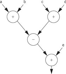
Q5-11 Draw the CDFG for the following C code before and after applying dead code elimination to the if statement:
#define DEBUG 0
proc1();
if (DEBUG) debug_stuff();
switch (foo) {
case A: a_case();
case B: b_case();
default: default_case();
}
Q5-12 Unroll the loop below:
Q5-13 Apply loop fusion or loop distribution to these code fragments as appropriate. Identify the technique you use and write the modified code.
a. for (i=0; i<N; i++)
z[i] = a[i] + b[i];
for (i=0; i<N; i++)
w[i] = a[i] − b[i];
b. for (i=0; i<N; i++) {
x[i] = c[i]*d[i];
y[i] = x[i] * e[i];
}
c. for (i=0; i<N; i++) {
for (j=0; j<M; j++) {
c[i][j] = a[i][j] + b[i][j];
x[j] = x[j] * c[i][j];
}
y[i] = a[i] + x[j];
}
Q5-14 Can you apply code motion to the following example? Explain.
for (i = 0; i < N; i++)
for (j = 0; j < M; j++)
z[i][j] = a[i] * b[i][j];
Q5-15 For each of the basic blocks of Q5-4, determine the minimum number of registers required to perform the operations when they are executed in the order shown in the code. (You can assume that all computed values are used outside the basic blocks, so that no assignments can be eliminated.)
Q5-16 For each of the basic blocks of Q5-4, determine the order of execution of operations that gives the smallest number of required registers. Next, state the number of registers required in each case. (You can assume that all computed values are used outside the basic blocks, so that no assignments can be eliminated.)
Q5-17 Draw a data flow graph for the code fragment of Example 5.6. Assign an order of execution to the nodes in the graph so that no more than four registers are required. Explain how you arrived at your solution using the structure of the data flow graph.
Q5-18 Determine the longest path through each code fragment, assuming that all statements can be executed in equal time and that all branch directions are equally probable.
a. if (i < CONST1) { x = a + b; }
else { x = c − d; y = e + f; }
b. for (i = 0; i < 32; i++)
if (a[i] < CONST2)
x[i] = a[i] * c[i];
c. if (a < CONST3) {
if (b < CONST4)
w = r + s;
else {
w = r − s;
x = s + t;
}
} else {
if (c > CONST5) {
w = r + t;
x = r − s;
y = s + u;
}
}
Q5-19 For each code fragment, list the sets of variable values required to execute each assignment statement at least once. Reaching all assignments may require multiple independent executions of the code.
a. if (a > 0)
x = 5;
else {
if (b < 0)
x = 7;
}
b. if (a == b) {
if (c > d)
x = 1;
else
x = 2;
x = x + 1;
}
Q5-20 Determine the shortest path through each code fragment, assuming that all statements can be executed in equal time and that all branch directions are equally probable. The first branch is always taken.
Q5-21 Write the branch tests for each conditional.
Q5-22 The loop appearing below is executed on a machine that has a 1-K-word data cache with four words per cache line.
a. How must x and a be placed relative to each other in memory to produce a conflict miss every time the inner loop’s body is executed?
b. How must x and a be placed relative to each other in memory to produce a conflict miss one out of every four times the inner loop’s body is executed?
c. How must x and a be placed relative to each other in memory to produce no conflict misses?
for (i = 0; i < 50; i++)
for (j = 0; j < 4; j++)
x[i][j] = a[i][j] * c[i];
Q5-23 Explain why the person generating clear-box program tests should not be the person who wrote the code being tested.
Q5-24 Find the cyclomatic complexity of the CDFGs for each of the code fragments given below.
a. if (a < b) {
if (c < d)
x = 1;
else
x = 2;
} else {
if (e < f)
x = 3;
else
x = 4;
}
b. switch (state) {
case A:
if (x = 1) { r = a + b; state = B; }
else { s = a − b; state = C; }
break;
case B:
s = c + d;
state = A;
break;
case C:
if (x < 5) { r = a − f; state = D; }
else if (x == 5) { r = b + d; state = A; }
else { r = c + e; state = D; }
break;
case D:
r = r + 1;
state = D;
break;
}
c. for (i = 0; i < M; i++)
for (j = 0; j < N; j++)
x[i][j] = a[i][j] * c[i];
Q5-25 Use the branch condition testing strategy to determine a set of tests for each of the following statements.
a. if (a < b || ptr1 == NULL) proc1();
else proc2();
b. switch (x) {
case 0: proc1(); break;
case 1: proc2(); break;
case 2: proc3(); break;
case 3: proc4(); break;
default; dproc(); break;
}
c. if (a < 5 && b > 7) proc1();
else if (a < 5) proc2();
else if (b > 7) proc3();
else proc4();
Q5-26 Find all the def-use pairs for each code fragment given below.
a. x = a + b;
if (x < 20) proc1();
else {
y = c + d;
while (y < 10)
y = y + e;
}
b. r = 10;
s = a − b;
for (i = 0; i < 10; i++)
x[i] = a[i] * b[s];
c. x = a − b;
y = c − d;
z = e − f;
if (x < 10) {
q = y + e;
z = e + f;
}
if (z < y) proc1();
Q5-27 For each of the code fragments of Q5-26, determine values for the variables that will cause each def-use pair to be exercised at least once.
Q5-28 Assume you want to use random tests on an FIR filter program. How would you know when the program under test is executing correctly?
Lab exercises
L5-1 Compare the source code and assembly code for a moderate-size program. (Most C compilers will provide an assembly language listing with the -S flag.) Can you trace the high-level language statements in the assembly code? Can you see any optimizations that can be done on the assembly code?
L5-2 Write C code for an FIR filter. Measure the execution time of the filter, either using a simulator or by measuring the time on a running microprocessor. Vary the number of taps in the FIR filter and measure execution time as a function of the filter size.
L5-3 Write C++ code for an FIR filter using a class to implement the filter. Implement as many member functions as possible as inline functions. Measure the execution time of the filter and compare to the C implementation.
L5-4 Generate a trace for a program using software techniques. Use the trace to analyze the program’s cache behavior.
L5-5 Use a cycle-accurate CPU simulator to determine the execution time of a program.
L5-6 Measure the power consumption of your microprocessor on a simple block of code.
L5-7 Use software testing techniques to determine how well your input sequences to the cycle-accurate simulator exercise your program.
L5-8 Generate a set of functional tests for a moderate-size program. Evaluate your test coverage in one of two ways: Have someone else independently identify bugs and see how many of those bugs your tests catch (and how many tests they catch that were not found by the human inspector); or inject bugs into the code and see how many of those are caught by your tests.