4
Failure Criterion: The Micromechanical Basis of Coulomb Criterion

Chapter 3 is focused on essential consequences of the tensor structures induced by contact friction in the pseudo-continuum, related to internal movements. Chapters 4, 5 and 6 are focused on another set of essential consequences, related to internal forces, and particularly the failure criterion.

Since the historical publication of Coulomb about two and a half centuries ago, the “Coulomb Failure Criterion” emerged progressively and stood out as a reference to efficiently describe the mechanical behavior at macro-scale of frictional materials in geomechanics, playing a key role in numerous methods for the design and verification of civil engineering works.

However, the direct link of general significance between this failure criterion and elementary physics of micromechanical behavior still remains to be established.

This direct link is the object of this chapter, at a critical state.

Under wide three-dimensional stress conditions, the eventuality of a failure criterion is investigated inside the macroscopic dissipation equation, under stationary specific volume condition.

The explicitly found minimum shear strength solution occurs to be the 3D pyramid of the Coulomb Failure Criterion. This Coulomb Criterion appears explicitly either as the least shear strength criterion or as the envelope of least dissipation criteria found under different sets of boundary conditions.

Moreover, this energy-based approach also provides a clear insight over the strain modes naturally attached to this Coulomb Failure Criterion, bringing a new perspective on the implementation of this criterion in plasticity.

Finally, considering the critical state as an asymptotic regime, the consequences of small deviations from the minimum resistance solution are analyzed. The resulting failure criterion, a kind of smoothed Coulomb Criterion pyramid, displays a shape not far from the shapes of experimental failure criteria measured in the past in extensive 3D testings.

4.1. Background and framework of the analysis

The concept of failure criterion, and specifically the Coulomb Criterion, plays a key role in Soil Mechanics and its applications in civil engineering (Figure 4.1)¹, particularly to design and verify geotechnical works with a specified safety margin against shear failure, such as:

– slope stability through limit equilibrium methods;
– active and passive thrusts and design of retaining structures;
– bearing capacity of foundations through plasticity methods.

In solid materials like concrete or rocks, “failure” corresponds to the development of microcracks and flaws up to the emergence of macro-scale discontinuities, and the Coulomb Criterion appears explicitly in the micromechanical analysis of the onset of microcrack propagation [LIN 80]. In geotechnical materials such as granular materials, already densely discontinuous even at small scale, the concept of “failure criterion” is different. Here, the “failure” is related either to stress conditions providing a maximum of shear resistance or to stress conditions making very large strains possible.

The “Coulomb Failure Criterion” we know today emerged progressively through successive works, first from Coulomb [COU 73], followed by Navier [NAV 33], Rankine [RAN 57], Mohr [MOH 00], Caquot [CAQ 34], Terzaghi [TER 48], and followers.

**Figure 4.1.** Coulomb Failure Criterion and key geomechanical issues in Civil Engineering. (a) Coulomb Failure Criterion. (b) Stability of slopes. (c) Thrusts on retaining structures. (d) Bearing capacity of foundations

However, as pointed out by Handin [HAN 69]: “The physics of the Coulomb equation is obscure…” Thus, a direct link of general reach between this failure criterion and elementary features of the mechanical behavior at micro-scale in geotechnical materials still remains to be established.

Since Coulomb’s publication, many investigations have tracked the role of physical contact sliding friction inside of the granular media macroscopic behavior. Despite remarkable advances such as Rowe “stress–dilatancy” theory (1962), reworked by Horne (1965–1969), or works by Cambou (1985), the subject still lacks an achieved clarification suited to general situations of practical interest, such as 3D failure criterion (or stress–strain relationship), which is the objective of this section.

4.2. Failure criterion at a critical state: the Coulomb Criterion

4.2.1. Specificity of “failure” under large shear strains – an analytical framework

When large shear strains develop in granular materials under monotonic conditions, volume changes, which usually denote the beginning of motion, fade and tend toward stationary specific volume conditions of motion: the “critical state” outlined earlier by Casagrande [CAS 36], later extended by Schofield and Wroth [SCH 80]. Indeed, if very large shear strains are compatible with the nature intrinsically discontinuous of these materials, volume changes are physically constrained by geometric restrictions: dilation is limited by the fact that particles shall remain in contact; contraction is limited by the steric arrangement of particles.

Thus, shear under large monotonic strains will be considered here as associated with the stationary specific volume condition, i.e. the trace of strain rate tensor is null

[4.1]

The common failure criteria are commonly represented by a surface in the principal stress space. In the present situation, the structure of the two available conditions, dissipation equation [1.30] and the above constant volume condition [4.1], shows that such a surface, if any, is conical, with the apex at the origin and with the isotropic stress line as the ternary symmetry axis.

However, as outlined in the previous simplified analysis of the subject [FRO 86], these two available conditions are insufficient to completely determine the failure criterion surface under common boundary conditions: an additional condition is required to “close” the problem, which may be represented as a functional relationship between the deviators of both stress and strain rate tensors, designated by “deviatoric relation.”

In our framework of simple coaxiality, this sought deviatoric relation may be written as a simple functional relationship between the two scalar parameters defining deviatoric stress state images (with 0 ≤ b ≤ 1 under our numbering convention σ₁ ≥ σ₂ ≥ σ₃ > 0), and deviatoric strain rate state images (with no special restriction here, as we consider simple coaxiality).

At this point it remains to be determined, within the mechanical behavior, what are the physical bases for such a “deviatoric relation”, and what it is precisely.

4.2.2. The criterion of least shear resistance

4.2.2.1. Framework and basic results

In this section, we investigate whether the shear resistance has a lower bound among all the possible solutions of the dissipation equation [1.30] near minimal dissipation with stationary specific volume.

In the space of principal stresses, if the surface of failure criterion is conical and regular, with ternary symmetry around the isotropic axis, the least resistance in stresses is the one achieving a minimum of Sup(σ₁, σ₂, σ₃)/Inf(σ₁, σ₂, σ₃). The principal stresses being ordered in descending order, this ratio becomes merely σ₁/σ₃, which may depend on deviatoric parameters {b, c}.

In terms of strain motions to be considered, among the six generally allowed strain modes (see section 1.3.4), two strain modes result in being discarded under stationary specific volume, on the condition of positive dissipation Tr{π} > 0 (Appendix A.4): these excluded modes are Mode I Reverse (−,−,+) and Mode II Reverse (−,+,+). Therefore, four strain modes remain to be investigated (Table 4.1).

The detailed analysis of these four modes is summarized in Appendix A.4.1. Figure 4.2 shows the map of allowed situations with stationary specific volume in the deviatoric plane {b, c}, with limitations due to the condition of no-tensile stresses (or no-tension).

**Figure 4.2.** *Mapping of Table 4.1 strain modes in the deviatoric plane {b, c}. (a) Ordered coaxiality domain. (b) Limitations resulting from the dissipation relation*

This analysis shows that, in all these allowed strain modes, based on the dissipation equation:

– The ratio σ₁/σ₃ may be expressed with the deviatoric parameters (b, c).
– This ratio is always found to be .
– The set of the results may be represented by a three-dimensional “surface of relative internal friction”, of which coordinates {x,y,z} are defined by (z coordinate definition being selected to avoid infinite branches, corresponding to crossing the limit of tensile stresses on σ₃)
[4.2]

– This surface, shown in Figure 4.3(a), is made up of a set of different sheets corresponding to the different allowed strain mode situations.
– These sheets either join along curvilinear ridges or wrinkles corresponding to crossing plane strain conditions (c = –1 for for , and c = 2 for = 0), or show crest lines z = 1 corresponding to infinite values of the ratio σ₁/σ₃ associated with reaching the limit of tensile stresses (σ₃/σ₁ = 0), and thalweg lines corresponding to the minimum values of the ratio σ₁/σ₃, all situated at z = 0.
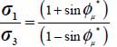
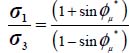
– The locus of points (b, c) corresponding to these minima, shown on the map of strain modes in Figure 4.3(b), constitutes the sought “deviatoric relation”, and generally corresponds only to plane strain upon the intermediate principal stress direction (c = 1/2, for = 0), for which stresses satisfy .
– Out of these plane strain conditions, the case of Mode I under axisymmetric stresses b = 0 (i.e. usual “triaxial” compression test) is part of this minima locus, for which a wide range of strain regimes satisfy this minimum (for −1 ≤ c ≤ 1/2), with the same stress relation .

**Figure 4.3.** Critical state least shear resistance solution and failure criterion (with associated micro-scale polarization features). (a) In the {b,c,z} coordinates space. (b) On the plane {b,c}: minimum solution “deviatoric relation.” (c) Resulting failure criterion (octahedral plane section): the Coulomb Criterion pyramid

– Out of these plane strain conditions, symmetrically the case of Mode II under axisymmetric stresses, b = 1 (i.e. “triaxial” extension test) is part of this minima locus, for which a wide range of strain regimes also satisfy this minimum (for ½ ≤ c ≤ 2), with the same stress relation .

4.2.2.2. Resulting failure criterion: the Coulomb Criterion

The corresponding failure criterion is

[4.3]

It is the pyramid of the Coulomb Criterion built with the angle images :

– This failure criterion is generally associated with plane strain appearing spontaneously upon the intermediate principal stress direction (Figure 4.3(c)). This explains why intermediate principal stress has disappeared in the criterion [4.3], despite the perfect symmetry of key relations [1.30] and [4.1]: as there is no mechanical work on this direction n°2 (since = 0), the corresponding principal stress σ₂ disappears from the work rate balance and derived relations:
– Apparent inter-granular friction angle takes a new physical significance from [4.3]: it is the constant volume internal friction φ_CV
[4.4]

– Difference between φ_CV and φ_μ (relation [1.19]) is clearly related to the parameter R representing an internal statistical disorder within the granular media in motion.
– Although the initial assumption considers general (disordered) simple coaxiality, the set of minimal solutions constituting the failure criterion are found to fully achieve ordered coaxiality.
– This least shear resistance failure criterion is found to be independent of boundary conditions’ particularities (provided that these boundary conditions allow the material motion to remain near minimal dissipation solutions).

4.2.3. Link with least dissipation criterion

As discussed above, the failure criterion for least shear resistance has been found, resulting from the dissipation equation, near minimal dissipation regimes. This section highlights the link between least shear resistance and least dissipation: if a criterion of least dissipation is investigated, it is found to correspond mostly with the criterion of least shear resistance. However, as the least dissipation analysis involves the boundary conditions, these must be specified. Such boundary conditions allow for coaxiality, maintain control of motion (quasi-equilibrium), maintain the material under controlled confinement, and allow for enough freedom in motion to leave the material to remain in the vicinity of “minimum dissipation” solutions.

Thus, in this section, we consider the following sets of controlled boundary conditions and variables:

– Boundary conditions “A” which can be called “controlled monotonic multi-axial compression” corresponding to classical testing procedures in 3D multi-axial testing [LAD 73, SHI 10, XIA 14] include also usual “triaxial compression” tests
[4.5a]
– Boundary conditions “B” which can be called “controlled monotonic multi-axial extension,” a kind of reciprocal of the preceding one, include also the “triaxial extension” tests
[4.5b]

In the Mohr circles plane of principal stresses σ₁, σ₂, σ₃, the above sets of boundary conditions, starting from an isotropic initial stress state σ₀, can be illustrated in Figure 4.4: the development of solicitations under boundary conditions A and B shows some similarity with the development of active and passive equilibriums.

**Figure 4.4.** *Investigated boundary conditions A and B*

Within the above framework, we show that physical bases for the sought deviatoric relation may also be attributed once again to the minimum energy dissipation rule: among all the solutions of the dissipation relation [1.30], with the stationary volume condition [4.1], we investigate the existence of a solution dissipating less energy than others.

However, absolute values in the dissipation relation have discontinuous derivatives, so a strategy has been adopted here to find that minimum value. For that, a reference solution is chosen, and the energy dissipation rate of any other solution is compared to the dissipation rate of reference solution under the same boundary conditions [4.5]: the ratio between both dissipation rates allows us to look for a possible minimum. The reference solution chosen for this purpose is the plane strain solution with images = 0 (so, images > 0 and images < 0, to get the positive dissipation rate).

Of the six generally allowed strain modes (see section 1.3.4), two results are discarded by the boundary conditions on the strain rate sign (either images > 0 or images < 0), and one is excluded by the positive dissipation condition and simultaneously boundary condition on the strain rate sign, for each of the boundary condition sets A and B. Therefore, only Modes I and II Direct, and one Transverse Mode remain for boundary conditions A and B (Table 4.2).

Mode designation	Signature	Restrictions of boundary conditions A	Restrictions of boundary conditions B
Mode I Direct	+,−,−	Allowed	Allowed
M. I Transverse	−,+,−	Discarded by bound. cond. > 0	Allowed
M. I Reverse	−,−,+	Excluded by positive dissipation condition and bound. cond. > 0	Excluded by positive dissipation condition and bound. cond. < 0
Mode II Direct	+,+,−	Allowed	Allowed
M. II Transverse	+,−,+	Allowed	Discarded by bound. cond. < 0
M. II Reverse	−,+,+	Discarded by bound. cond. > 0	Discarded by bound. cond. < 0

4.2.3.1. Basic results

Boundary conditions A

A detailed analysis of Appendix A.4.2 shows the following for all three allowable strain mode situations:

– The energy rate dissipated by any solution Tr{π}, and the energy rate dissipated by the reference solution Tr{π₀}, can be expressed exclusively in function of deviatoric parameters (b and c), and fixed boundary conditions ( and σ₃); their ratio Tr{π}/Tr{π₀} depends only on deviatoric parameters b and c.
– This ratio is found as , i.e. there is no allowable solution dissipating less energy than the reference plane strain solution.
– The set of results can be represented by a three-dimensional “surface of relative dissipation”, for which coordinates {x,y,z} are defined by (z coordinate definition being selected to avoid infinite branches)
– This surface, shown in Figure 4.5(a), is constituted of a set of different sheets corresponding to the different allowed strain mode situations.
– These sheets either join along curvilinear ridges or wrinkles corresponding to crossing plane strain conditions (c = –1 for = 0, c = ½ for = 0, and c = 2 for = 0), or show crest lines z = 1 corresponding to infinite values of the ratio Tr{π}/Tr{π₀} associated with reaching the limit of tensile stresses (σ₃/σ₁ = 0), and thalweg lines corresponding to minimum values of the ratio Tr{π}/Tr{π₀}, all situated at z = 0.
– The locus of points (b, c) corresponding to these minima, displayed on the map of strain modes in Figure 4.5(b), constitutes the sought “deviatoric relation”, and generally corresponds only to plane strain upon the intermediate principal stress direction (c = 1/2, for = 0), for which stresses satisfy .
– Out of these plane strain conditions, the case of Mode I under axisymmetric stresses b = 0 (i.e. usual “triaxial” compression test) remains a part of this minima locus, for which a wide range of strain regimes do satisfy this minimum (for –1 ≤ c ≤ ½), with the same stress relation
– Out of these plane strain conditions, another case of Mode II under axisymmetric stresses b = 1, (i.e. “triaxial” extension test) is not part of this minimal dissipation locus, although in this case the stress relation is still satisfied.

**Figure 4.5.** Least dissipation criterion for boundary conditions A. (a) In the {b,c,z} coordinates space. (b) On the {b,c} diagram: minimum solution “deviatoric relation.” (c) Resulting failure criterion (octahedral plane section): the Coulomb Criterion pyramid

Boundary conditions B

A similar detailed analysis for all three allowable strain modes situations is summarized in Appendix A.4.2; however, in this situation, the discussion is more delicate than the above, because the confining stress σ₃ is left unbounded. Nevertheless, the results rather show similar main trends and features, with some differences:

– out of the predominant plane strain conditions, this time the case of Mode II under axisymmetric stresses b = 1 (i.e. “triaxial” extension test) is part of this least dissipation locus;
– symmetrically, the case of Mode I under axisymmetric stresses (i.e. classical “triaxial” compression tests) is no longer part of this minimum dissipation locus, although in this case the stress relation is still satisfied.

4.2.3.2. Comparison with the least shear resistance criterion

The above results are shown in Figure 4.6: in the pseudo-continuum representation, within the tensor structures induced by contact friction and condensed into the dissipation equation [1.30], the Coulomb Criterion explicitly appears either as the least shear strength criterion or as the envelope of least dissipation criterions found under different sets of boundary conditions.

Basic analytical reasons for this kind of equivalence may be found in the structure of the work rate of internal forces, here equal to the dissipation rate in the dissipation relation, so the least dissipation is also the minimum of this work rate of internal forces:

– Under plane strain ( = 0) and stationary specific volume (), the work rate of internal forces may be written in specific forms related to each set of boundary conditions A and B, isolating the variables set as constants for each set of boundary conditions:

Thus, under plane strain, the minimum of dissipation is equivalent to the minimum of shear resistance: minimum of the ratio σ₁/σ₃ for boundary conditions A, and a maximum of the ratio σ₃/σ₁ for boundary conditions B.

**Figure 4.6.** *The link between least shear strength and least dissipation criteria (with their respective deviatoric relations)*

– Under asymmetric stresses b = 0 (i.e. σ₂ = σ₃) in Mode I and stationary specific volume (), the internal work rate may be written in a similar way, but the following are only for boundary conditions A:

Thus, for axisymmetric stress conditions b = 0, the minimum of dissipation is equivalent to the minimum of the ratio σ₁ / σ₃ for boundary conditions A; however, this equivalence cannot be written here for boundary conditions B, which is the reason this part of the criterion is no longer a part of least dissipation solutions under boundary conditions B.

– Under axisymmetric stresses b = 1 (i.e. σ₁ = σ₂) in Mode II, a symmetrical analysis explains why it is part of least dissipation solutions for boundary conditions B, but not for boundary conditions A.

The practical consequence of this situation is that, under given experimental boundary conditions allowing the material to come close to minimal dissipation conditions, the “critical state failure criterion” observed may not display some part of the criterion (case of edge strain regimes under axisymmetric stresses excluded above), depending on the kind of boundary condition imposed.

4.2.3.4. Relative configuration of internal actions, stresses, and strain rates

Figure 4.7 shows the relative configuration of the three tensors (normalized with our tensor norm N for this comparison) π, σ, and images associated with this failure criterion.

**Figure 4.7.** *Relative arrangement of tensors σ, , and π, for critical state failure criterion. (a) Projections on an octahedral plane. (b) On the “unit ball” (octahedron) of tensorial norm N*

– As projected onto the octahedral plane (Figure 4.7(a)), the geometric figure associated with results from the stationary volume condition [4.1], the one associated with π results from the dissipation relation [1.30], and the one associated with σ is the failure criterion [4.3].
– On the unit ball (octahedron) of our norm N, inherited from the analysis of discontinuous granular mass, the relative arrangement is shown in Figure 4.7(b).

4.2.4. Incidence of small deviations from least shear resistance solution

The critical state can be considered as an asymptotic regime, so experimental data may still include some remaining deviations from that asymptotic minimal solution. If a given “deviatoric relation” b = f(c) is considered with some small deviations from minimal solution, the resulting failure criterion may be computed by injecting the numerical values {b, c} in the principal stress ratio relations detailed in Appendix A.4.1.

Figure 4.8(a) shows such a curvilinear “deviatoric relation” (see Appendix A.4.3) designed to secure deviations within 6% on the principal stress ratio, as compared with the Coulomb Criterion. The resulting failure criterion (Figure 4.8(b)) appears as made by smooth convex conical surfaces with rounded apexes, separated by a slightly non-convex undulation corresponding to the plane strain mode, at the border between Modes I and II.

That shape is quite close to the shapes of experimental failure criteria measured earlier in extensive 3D testings [LAD 73, ART 77], displaying similar slight undulations in some diagrams.

This general shape, made of convex sheets corresponding to each 3D strain mode in Mode I or II, separated by a non-convexity corresponding to crossing the border mode in plane strain between two 3D strain modes, results from the general features of minimal dissipation modes (see Chapter 1): the set of solutions for minimum dissipation is continuous, but only piecewise convex (each convex subset corresponding separately to each 3D mode).

Note that the Coulomb Criterion pyramid (Figure 4.3), among all allowable solutions of the dissipation relation [1.30], is the only solution achieving complete convexity, as well as being ordered coaxially. It may also be observed how these macroscopic features are naturally associated with micro-scale polarization patterns of elementary contacts sliding motions (Figures 4.3, 4.5, and 4.8) using the present dissipative approach.

**Figure 4.8.** Critical state failure criterion – incidence of small deviations from minimal solution. (a) Assumed “deviatoric relation.” (b) Resulting failure criterion. For a color version of the figure, please see www.iste.co.uk/frossard/geomaterials.zip

Mode designation	Mode I Direct	M. I Transverse	Mode II Direct	M. II Transverse
Signature	+,−,−	−,+,−	+,+,−	+,−,+