For a vector editor, one of the most important bitmap-related capabilities is converting bitmap objects to vectors (tracing) and vice versa (bitmap export). Inkscape offers rich and powerful tools for these conversions, which the rest of this chapter will cover in detail.
The most straightforward approach to creating vector art from a bitmap image does not involve any tools except those we already know. Just switch to the Pen tool (14.1 The Pen Tool), zoom in on your bitmap, and do a series of clicks around or along an area that you want to turn into a vector path, then double-click or press  to finish the path. Use click-and-release in a sharp corner to create a cusp node; for smooth curved edges, use a series of click-and-drags in critical nodes:
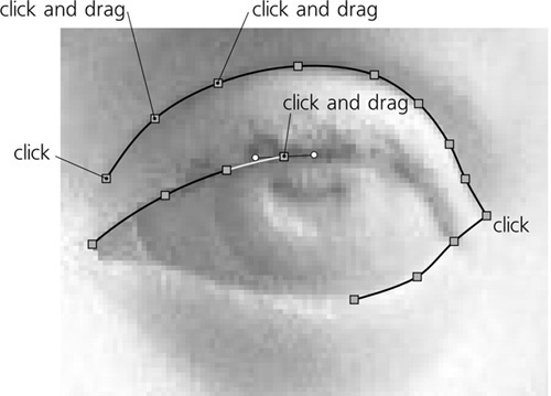
You can vary the density of your clicks depending on how precisely you want to trace a specific area. If you want the shape to be extra smooth, switch to the Spiro mode (13.1.7 Spiro Spline); in this mode, it does not matter in which direction you drag after clicking, just as long as you drag a bit somewhere to create a smooth node. If you’re tracing a polygon without any curves at all, it is convenient to use the Straight lines mode so that an accidental drag does not create an undesired smooth node.
While this technique may seem time-consuming at first, once you get the hang of it, you will be able to trace complex art very quickly. Like any manual technique, its main advantage is the complete creative control—you decide what parts to trace and what to ignore, how to simplify complex shapes, where to diverge from the bitmap blueprint, and where to place each node. Depending on your skill, the result will likely look much more satisfying than either an automatic trace or a fully manual drawing.
Inkscape’s tool for automatic bitmap tracing is very powerful; based on the standalone Potrace open source tracer (http://potrace.sourceforge.net), it is acknowledged to be one of the best tools of its kind in modern vector editors. With it, you can trace anything from a simple black-and-white logo that needs just a few nodes to a complex photo that produces dozens of colored paths with thousands of nodes.
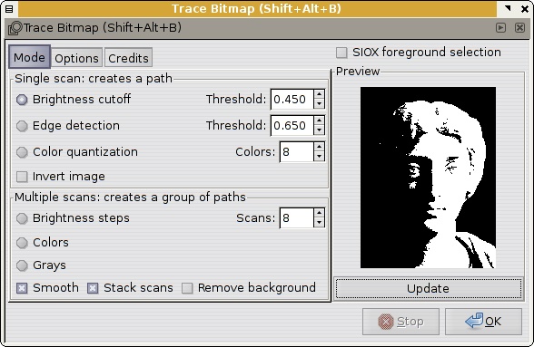
The Trace Bitmap dialog ( ) has two main areas: the options panel on the left and the preview panel on the right. Note, however, that the preview panel does not show you the traced vector path (that may be time-consuming to create); instead, you see the bitmap you’re tracing with all the color reduction and filtering steps as specified in the options panel. To update the preview after the options have changed, click Update.
To perform the actual trace of the selected bitmap object, click OK. For a large bitmap, this may be slow; watch the status bar for progress messages. You can interrupt tracing at any time by clicking the Stop button.
The Mode tab of the dialog chooses the principal mode of operation of the tracing tool. The available modes are divided into two groups: the single-scan modes create a single path, while the multiple-scan modes create multiple paths (grouped together).
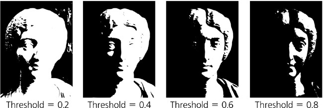
Brightness cutoff is the simplest and most common approach to tracing a path: The resulting path covers anything that is darker than the threshold you set. This trace path, while a single object, can consist of multiple nonoverlapping subpaths (12.1.1 Subpaths). The Threshold is set as a fraction of the entire brightness range of the image; for example, when set to 0.6, the trace path covers all the areas in the darkest 60 percent of the image. If you click Invert, the meaning of Threshold is inverted (i.e., the path will cover the brightest 40 percent of the image).
Usually, this is the best tracing mode for simple monochrome shapes such as logos, text, vignettes, and so on.
Even if the bitmap you’re tracing is a rendition of a vector path, the trace will never exactly reproduce that original path. Rendering a vector into a bitmap always incurs some loss of information, and Inkscape’s tracer cannot restore this lost information other than by guessing. Although it is generally pretty good at it, there will be cases where you will be disappointed by its failure to recognize some features (arcs, straight lines, corners) that you can easily “see” in the bitmap. This is especially evident when tracing low-resolution bitmaps or those containing text.
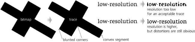
Perhaps the best piece of advice in this situation is to obtain the highest possible resolution bitmap. It is nearly impossible to get a decent trace from a bitmap where some crucial features are several pixels across; tracing a higher-resolution version of an image often makes a big difference. Also, you can try to adjust the Threshold and experiment with the contents of the Options page of the dialog (it applies to all modes, both single-scan and multiple-scan):
The Suppress speckles option removes any color blobs that are smaller than the specified number of pixels across. This suppresses creating small superfluous subpaths when tracing dirty or “dithered” bitmaps.
Increasing the Smooth corners parameter makes the trace algorithm less inclined to recognize sharp corners in the image. This may be useful when tracing a naturally smooth shape from a highly pixelated, low-resolution bitmap where you don’t want accidental pixel cusps to become sharp corners in the traced path. Conversely, lowering this parameter is appropriate when you are tracing geometric shapes without any curved lines; when Smooth corners is zero, the resulting path almost entirely consists of straight line segments with cusp nodes between them.
The Optimize paths parameter tries to reduce the number of nodes in the trace path, much like the Simplify command does (12.3 Simplifying). Raising this value decreases the number of nodes you get, but it also increases the chance of introducing visible distortions or losing some important details of the shape.
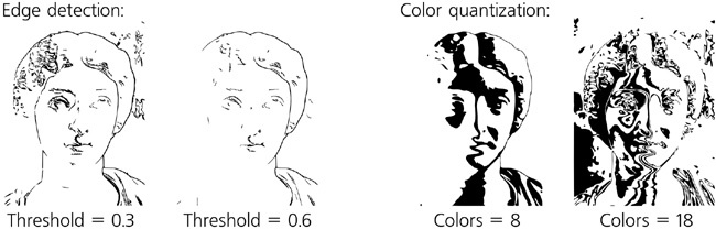
The Edge detection mode applies the edge detection filter to the bitmap before tracing it. As a result, the trace path will contain narrow strips that follow the color boundaries in the source bitmap. The lower the Threshold is, the more edges will be detected and traced.
The Color quantization mode first quantizes (divides) the image into the given number of areas (Colors), each with its own dominant color, much like when reducing a full-color image to a fixed palette using a bitmap editor. It then traces every other such area, which results in a stripped appearance for color gradients.
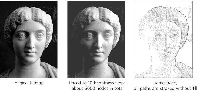
Like the Color quantization mode we’ve just seen, each multiple-scan mode starts by quantizing the image into the given number of areas (specified by Scans). It then traces each area separately, assigns an appropriate color or gray level to the trace path, and groups all such paths together. With a sufficient number of quantization steps, the result may look very similar to the original bitmap, faithfully reproducing its color gradients, blur, natural textures, and so on.
The three multiple-scan modes differ only in the way the image is quantized. The Brightness steps option is the best one for grayscale images; it ignores any hue or saturation differences and groups pixels into areas based solely on their brightness (Figure 18-14). The Colors mode considers all aspects of the colors when performing quantization, which results in the most faithful reproduction of full-color images (see Figure 14 on the color insert). Finally, the Grays option works the same as Colors, except that the resulting paths are painted with approximating shades of gray instead of the original colors.
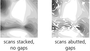
The Smooth option applies a certain amount of blur to the image before quantizing it; this may produce better results in complex photographic images. The Stack scans option is best kept on; it makes sure that each area’s path covers not only that area but also all areas below it in z-order, which means there will be no gaps between the scans:
The Remove background option simply removes the bottommost scan path from the group, which is useful when you are tracing a photo of something on a flat-color background and want the result to only contain the object itself, not the background.