
OTHER TECHNIQUES
14.2Compositing / Blending / Transparency
14.3User-Defined Clipping Planes
14.6Noise Application – Marble
14.8Noise Application – Clouds
14.9Noise Application – Special Effects

In this chapter we explore a variety of techniques utilizing the tools we have learned throughout the book. Some we will develop fully, while for others we will offer a more cursory description. Graphics programming is a huge field, and this chapter is by no means comprehensive, but rather an introduction to just a few of the creative effects that have been developed over the years.
14.1FOG
Usually when people think of fog, they think of early misty mornings with low visibility. In truth, atmospheric haze (such as fog) is more common than most of us think. The majority of the time, there is some degree of haze in the air, and although we have become accustomed to seeing it, we don’t usually realize it is there. So we can enhance the realism in our outdoor scenes by introducing fog—even if only a small amount.
Fog also can enhance the sense of depth. When close objects have better clarity than distant objects, it is one more visual cue that our brains can use to decipher the topography of a 3D scene.
Figure 14.1
Fog: blending based on distance.
There are a variety of methods for simulating fog, from very simple ones to sophisticated models that include light scattering effects. However, even very simple approaches can be effective. One such method is to blend the actual pixel color with another color (the “fog” color, typically gray or bluish-gray—also used for the background color), based on the distance the object is from the eye.
Figure 14.1 illustrates the concept. The eye (camera) is shown at the left, and two red objects are placed in the view frustum. The cylinder is closer to the eye, so it is mostly its original color (red); the cube is further from the eye, so it is mostly fog color. For this simple implementation, virtually all of the computations can be performed in the fragment shader.
Program 14.1 shows the relevant code for a very simple fog algorithm that uses a linear blend from object color to fog color based on the distance from the camera to the pixel. Specifically, this example adds fog to the height mapping example from Program 10.4.
Program 14.1 Simple Fog Generation

The variable fogColor specifies a color for the fog. The variables fogStart and fogEnd specify the range (in eye space) over which the output color transitions from object color to fog color, and can be tuned to meet the needs of the scene. The percentage of fog mixed with the object color is calculated in the variable fogFactor, which is the ratio of how close the vertex is to fogEnd to the total length of the transition region. The GLSL clamp() function is used to restrict this ratio to being between the values 0.0 and 1.0. The GLSL mix() function then returns a weighted average of fog color and object color, based on the value of fogFactor. Figure 14.2 shows the addition of fog to a scene with height mapped terrain. (A rocky texture from [LU16] has also been applied.)
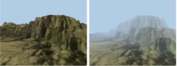
Figure 14.2
Fog example.
14.2COMPOSITING / BLENDING / TRANSPARENCY
We have already seen a few examples of blending—in the supplementary notes for Chapter 7, and just previously in our implementation of fog. However, we haven’t yet seen how to utilize the blending (or compositing) capabilities that follow after the fragment shader during pixel operations (recall the pipeline sequence shown in Figure 2.2). It is there that transparency is handled, which we look at now.
Throughout this book we have made frequent use of the vec4 data type, to represent 3D points and vectors in a homogeneous coordinate system. You may have noticed that we also frequently use a vec4 to store color information, where the first three values consist of red, green, and blue, and the fourth element is—what?
The fourth element in a color is called the alpha channel, and specifies the opacity of the color. Opacity is a measure of how non-transparent the pixel color is. An alpha value of 0 means “no opacity,” or completely transparent. An alpha value of 1 means “fully opaque,” not at all transparent. In a sense, the “transparency” of a color is 1-α, where α is the value of the alpha channel.
Recall from Chapter 2 that pixel operations utilize the Z-buffer, which achieves hidden surface removal by replacing an existing pixel color when another object’s location at that pixel is found to be closer. We actually have more control over this process—we may choose to blend the two pixels.
When a pixel is being rendered, it is called the “source” pixel. The pixel already in the frame buffer (presumably rendered from a previous object) is called the “destination” pixel. OpenGL provides many options for deciding which of the two pixels, or what sort of combination of them, ultimately is placed in the frame buffer. Note that the pixel operations step is not a programmable stage—so the OpenGL tools for configuring the desired compositing are found in the C++ application, rather than in a shader.
The two OpenGL functions for controlling compositing are glBlendEquation(mode) and glBlendFunc(srcFactor, destFactor). Figure 14.3 shows an overview of the compositing process.
The compositing process works as follows:
1.The source and destination pixels are multiplied by source factor and destination factor respectively. The source and destination factors are specified in the blendFunc() function call.
Figure 14.3
OpenGL compositing overview.
2.The specified blendEquation is then used to combine the modified source and destination pixels to produce a new destination color. The blend equation is specified in the glBlendEquation() call.
The most common options for glBlendFunc() parameters (i.e., srcFactor and destFactor) are shown in the following table:
Those options that indicate a “blendColor” (GL_CONSTANT_COLOR, etc.) require an additional call to glBlendColor() to specify a constant color that will be used to compute the blend function result. There are a few additional blend functions that aren’t shown in the previous list.
The possible options for the glBlendEquation() parameter (i.e., mode) are as follows:
| mode | blended color |
| GL_FUNC_ADD | result = sourceRGBA + destinationRGBA |
| GL_FUNC_SUBTRACT | result = sourceRGBA – destinationRGBA |
| GL_FUNC_REVERSE_SUBTRACT | result = destinationRGBA – sourceRGBA |
| GL_MIN | result = min(sourceRGBA, destinationRGBA) |
| GL_MAX | result = max(sourceRGBA, destinationRGBA) |
The glBlendFunc() defaults are GL_ONE (1.0) for srcFactor and GL_ZERO (0.0) for destFactor. The default for glBlendEquation() is GL_FUNC_ADD. Thus, by default, the source pixel is unchanged (multiplied by 1), the destination pixel is scaled to 0, and the two are added—meaning that the source pixel becomes the frame buffer color.
There are also the commands glEnable(GL_BLEND) and glDisable(GL_BLEND), which can be used to tell OpenGL to apply the specified blending, or to ignore it.
We won’t illustrate the effects of all of the options here, but we will walk through some illustrative examples. Suppose we specify the following settings in the C++/OpenGL application:
•glBlendFunc(GL_SRC_ALPHA, GL_ONE_MINUS_SRC_ALPHA)
•glBlendEquation(GL_FUNC_ADD)
Compositing would proceed as follows:
1.The source pixel is scaled by its alpha value.
2.The destination pixel is scaled by 1-srcAlpha (the source transparency).
3.The pixel values are added together.
For example, if the source pixel is red, with 75% opacity: [1, 0, 0, 0.75], and the destination pixel contains completely opaque green: [0, 1, 0, 1], then the result placed in the frame buffer would be:
srcPixel * srcAlpha = [0.75, 0, 0, 0.5625]
destPixel * (1-srcAlpha) = [0, 0.25, 0, 0.25]
resulting pixel = [0.75, 0.25, 0, 0.8125]
That is, predominantly red, with some green, and mostly solid. The overall effect of the settings is to let the destination show through by an amount corresponding to the source pixel’s transparency. In this example, the pixel in the frame buffer is green, and the incoming pixel is red with 25% transparency (75% opacity). So some green is allowed to show through the red.
It turns out that these settings for blend function and blend equation work well in many cases. Let’s apply them to a practical example in a scene containing two 3D models: a torus and a pyramid in front of the torus. Figure 14.4 shows such a scene, on the left with an opaque pyramid, and on the right with the pyramid’s alpha value set to 0.8. Lighting has been added.
For many applications—such as creating a flat “window” as part of a model of a house—this simple implementation of transparency may be sufficient. However, in the example shown in Figure 14.4, there is a fairly obvious inadequacy. Although the pyramid model is now effectively transparent, an actual transparent pyramid should reveal not only the objects behind it, but also its own back surfaces.
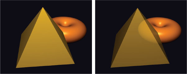
Figure 14.4
Pyramid with alpha=1.0 (left), and alpha=0.8 (right).
Actually, the reason that the back faces of the pyramid did not appear is because we enabled back-face culling. A reasonable idea might be to disable back-face culling while drawing the pyramid. However, this often produces other artifacts, as shown in Figure 14.5 (on the left). The problem with simply disabling back-face culling is that the effects of blending depend on the order that surfaces are rendered (because that determines the source and destination pixels), and we don’t always have control over the rendering order. It is generally advantageous to render opaque objects first, as well as objects that are in the back (such as the torus) before any transparent objects. This also holds true for the surfaces of the pyramid, and in this case the reason that the two triangles comprising the base of the pyramid appear different is that one of them was rendered before the front of the pyramid and one was rendered after. Artifacts such as this are sometimes called “ordering” artifacts, and they can manifest in transparent models because we cannot always predict the order in which its triangles will be rendered.
We can solve the problem in our pyramid example by rendering the front and back faces separately, ourselves, starting with the back faces. Program 14.2 shows the code for doing this. We specify the alpha value for the pyramid by passing it to the shader program in a uniform variable, then apply it in the fragment shader by substituting the specified alpha into the computed output color.
Note also that for lighting to work properly, we must flip the normal vector when rendering the back faces. We accomplish this by sending a flag to the vertex shader, where we then flip the normal vector.
Program 14.2 Two-Pass Blending for Transparency
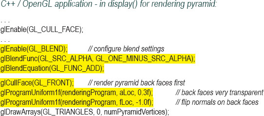
The result of this “two-pass” solution is shown in Figure 14.5, on the right.
Although it works well here, the two-pass solution shown in Program 14.2 is not always adequate. For example, some more complex models may have hidden surfaces that are front-facing, and if such an object were made transparent, our algorithm would fail to render those hidden front-facing portions of the model. Alec Jacobson describes a five-pass sequence that works in a large number of cases [JA12].
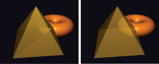
Figure 14.5
Transparency and back faces: ordering artifacts (left) and two-pass correction (right).
14.3USER-DEFINED CLIPPING PLANES
OpenGL includes the capability to specify clipping planes beyond those defined by the view frustum. One use for a user-defined clipping plane is to slice a model. This makes it possible to create complex shapes by starting with a simple model and slicing sections off of it.
A clipping plane is defined according to the standard mathematical definition of a plane:
ax + by + cz + d = 0
where a, b, c, and d are parameters defining a particular plane in 3D space with X, Y, and Z axes. The parameters represent a vector (a,b,c) normal to the plane, and a distance d from the origin to the plane. Such a plane can be specified in the vertex shader using a vec4, as follows:
vec4 clip_plane = vec4(0.0, 0.0, -1.0, 0.2);
This would correspond to the plane:
(0.0) x + (0.0) y + (-1.0) z + 0.2 = 0
The clipping can then be achieved, also in the vertex shader, by using the built-in GLSL variable gl_ClipDistance[ ], as in the following example:
gl_ClipDistance[0] = dot(clip_plane.xyz, vertPos) + clip_plane.w;
In this example, vertPos refers to the vertex position coming into the vertex shader in a vertex attribute (such as from a VBO); clip_plane was defined above. We then compute the signed distance from the clipping plane to the incoming vertex (shown in Chapter 3), which is either 0 if the vertex is on the plane, or is negative or positive depending on which side of the plane the vertex lies. The subscript on the gl_ClipDistance array enables multiple clipping distances (i.e., multiple planes) to be defined. The maximum number of user clipping planes that can be defined depends on the graphics card’s OpenGL implementation.
User-defined clipping must then be enabled in the C++/OpenGL application. There are built-in OpenGL identifiers GL_CLIP_DISTANCE0, GL_CLIP_DISTANCE1, and so on, corresponding to each gl_ClipDistance[ ] array element. The 0th user-defined clipping plane can be enabled, for example, as follows:
glEnable(GL_CLIP_DISTANCE0);
Figure 14.6
Clipping a torus.
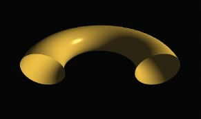
Figure 14.7
Clipping with back faces.
Applying the previous steps to our lighted torus results in the output shown in Figure 14.6, in which the front half of the torus has been clipped. (A rotation has also been applied to provide a clearer view.)
It may appear that the bottom portion of the torus has also been clipped, but that is because the inside faces of the torus were not rendered. When clipping reveals the inside surfaces of a shape, it is necessary to render them as well, or the model will appear incomplete (as it does in Figure 14.6).
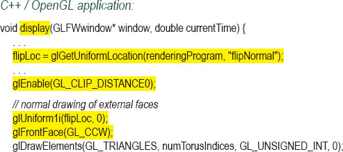
Rendering the inner surfaces requires making a second call to gl_DrawArrays(), with the winding order reversed. Additionally, it is necessary to reverse the surface normal vector when rendering the back-facing triangles (as was done in the previous section). The relevant modifications to the C++ application and the vertex shader are shown in Program 14.3, with the output shown in Figure 14.7.
Program 14.3 Clipping with Back Faces
14.43D TEXTURES
Whereas 2D textures contain image data indexed by two variables, 3D textures contain the same type of image data, but in a 3D structure that is indexed by three variables. The first two dimensions still represent width and height in the texture map; the third dimension represents depth.
Because the data in a 3D texture is stored in a similar manner as for 2D textures, it is tempting to think of a 3D texture as a sort of 3D “image.” However, we generally don’t refer to 3D texture source data as a 3D image, because there are no commonly used image file formats for this sort of structure (i.e., there is nothing akin to a 3D JPEG, at least not one that is truly three-dimensional). Instead, we suggest thinking of a 3D texture as a sort of substance into which we will submerge (or “dip”) the object being textured, resulting in the object’s surface points obtaining their colors from the corresponding locations in the texture. Alternatively, it can be useful to imagine that the object is being “carved” out of the 3D texture “cube,” much like a sculptor carves a figure out of a single solid block of marble.
OpenGL has support for 3D texture objects. In order to use them, we need to learn how to build the 3D texture and how to use it to texture an object.
Unlike 2D textures, which can be built from standard image files, 3D textures are usually generated procedurally. As was done previously for 2D textures, we decide on a resolution—that is, the number of texels in each dimension. Depending on the colors in the texture, we may build a three-dimensional array containing those colors. Alternatively, if the texture holds a “pattern” that could be utilized with various colors, we might instead build an array that holds the pattern, such as with 0s and 1s.
For example, we can build a 3D texture that represents horizontal stripes by filling an array with 0s and 1s corresponding to the desired stripe pattern. Suppose that the desired resolution of the texture is 200x200x200 texels, and the texture is comprised of alternating stripes that are each 10 texels high. A simple function that builds such a structure by filling an array with appropriate 0s and 1s in a nested loop (assuming in this case that width, height, and depth variables are each set to 200) would be as follows:
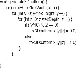
The pattern stored in the tex3Dpattern array is illustrated in Figure 14.8 with the 0s rendered in blue and the 1s rendered in yellow.
Texturing an object with the striped pattern as shown in Figure 14.8 requires the following steps:
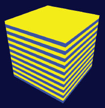
Figure 14.8
Striped 3D texture pattern.
1.generating the pattern as already shown
2.using the pattern to fill a byte array of desired colors
3.loading the byte array into a texture object
4.deciding on appropriate 3D texture coordinates for the object vertices
5.texturing the object in the fragment shader using an appropriate sampler
Texture coordinates for 3D textures range from 0 to 1, in the same manner as for 2D textures.
Interestingly, step #4 (determining 3D texture coordinates) is usually a lot simpler than one might initially suspect. In fact, it is usually simpler than for 2D textures! This is because (in the case of 2D textures) since a 3D object was being textured with a 2D image, we needed to decide how to “flatten” the 3D object’s vertices (such as by UV-mapping) to create texture coordinates. But when 3D texturing, both the object and the texture are of the same dimensionality (three). In most cases, we want the object to reflect the texture pattern, as if it were “carved” out of it (or dipped into it). So the vertex locations themselves serve as the texture coordinates! Usually all that is necessary is to apply some simple scaling to ensure that the object’s vertices’ location coordinates map to the 3D texture coordinates’ range [0..1].
Since we are generating the 3D texture procedurally, we need a way of constructing an OpenGL texture map out of generated data. The process for loading data into a texture is similar to what we saw earlier in Section 5.12. In this case, we fill a 3D array with color values, then copy them into a texture object.
Program 14.4 shows the various components for achieving all of the previous steps in order to texture an object with blue and yellow horizontal stripes from a procedurally built 3D texture. The desired pattern is built in the generate3Dpattern() function, which stores the pattern in an array named “tex3Dpattern”. The “image” data is then built in the function fillDataArray(), which fills a 3D array with byte data corresponding to the RGB colors R, G, B, and A, each in the range [0..255], according to the pattern. Those values are then copied into a texture object in the load3DTexture() function.
Program 14.4 3D Texturing: Striped Pattern
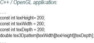
In the C++/OpenGL application, the load3Dtexture() function loads the generated data into a 3D texture. Rather than using SOIL2 to load the texture, it makes the relevant OpenGL calls directly, in a manner similar to that explained earlier in Section 5.12. The image data is expected to be formatted as a sequence of bytes corresponding to RGBA color components. The function fillDataArray() does this, applying the RGB values for yellow and blue corresponding to the striped pattern built by the generate3Dpattern() function and held in the tex3Dpattern array. Note also the specification of texture type GL_TEXTURE_3D in the display() function.
Since we wish to use the object’s vertex locations as texture coordinates, we pass them through from the vertex shader to the fragment shader. The fragment shader then scales them so that they are mapped into the range [0..1] as is standard for texture coordinates. Finally, 3D textures are accessed via a sampler3D uniform, which takes three parameters instead of two. We use the vertex’s original X, Y, and Z coordinates, scaled to the correct range, to access the texture. The result is shown in Figure 14.9.
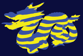
Figure 14.9
Dragon object with 3D striped texture.
More complex patterns can be generated by modifying generate3Dpattern(). Figure 14.10 shows a simple change that converts the striped pattern to a 3D checkerboard. The resulting effect is then shown in Figure 14.11. It is worth noting that the effect is very different from what the case would be if the dragon’s surface had been textured with a 2D checkerboard texture pattern. (See Exercise 14.3.)
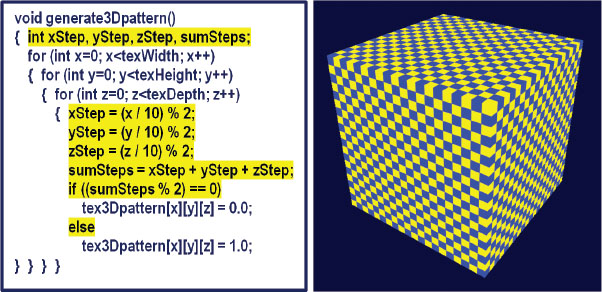
Figure 14.10
Generating a checkerboard 3D texture pattern.
Many natural phenomena can be simulated using randomness, or noise. One common technique, Perlin Noise [PE85], is named after Ken Perlin, who in 1997 received an Academy Award1 for developing a practical way to generate and use 2D and 3D noise. The procedure described here is based on Perlin’s method.
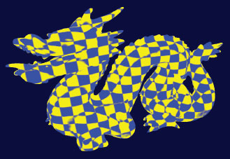
Figure 14.11
Dragon with 3D checkerboard texture.
There are many applications of noise in graphics scenes. A few common examples are clouds, terrain, wood grain, minerals (such as veins in marble), smoke, fire, flames, planetary surfaces, and random movements. In this section, we focus on generating 3D textures containing noise, and then subsequent sections illustrate using the noise data to generate complex materials such as marble and wood, and to simulate animated cloud textures for use with a cube map or skydome. A collection of spatial data (e.g., 2D or 3D) that contains noise is sometimes referred to as a noise map.
We start by constructing a 3D texture map out of random data. This can be done using the functions shown in the previous section, with a few modifications. First, we replace the generate3Dpattern() function from Program 14.4 with the following simpler generateNoise() function:

Next, the fillDataArray() function from Program 14.4 is modified so that it copies the noise data into the byte array in preparation for loading into a texture object, as follows:
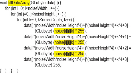
The rest of Program 14.4 for loading data into a texture object and applying it to a model is unchanged. We can view this 3D noise map by applying it to our simple cube model, as shown in Figure 14.12. In this example, noiseHeight = noiseWidth = noiseDepth = 256.
This is a 3D noise map, although it isn’t a very useful one. As is, it is just too noisy to have very many practical applications. To make more practical, tunable noise patterns, we will replace the fillDataArray() function with different noise-producing procedures.

Figure 14.12
Cube textured with 3D noise data.
Suppose that we fill the data array by “zooming in” to a small subsection of the noise map illustrated in Figure 14.12, using indexes made smaller by integer division. The modification to the fillDataArray() function is shown below. The resulting 3D texture can be made more or less “blocky” depending on the “zooming” factor used to divide the index. In Figure 14.13, the textures show the result of zooming in by dividing the indices by zoom factors 8, 16, and 32 (left to right respectively).
Figure 14.13
“Blocky” 3D noise maps with various “zooming in” factors.
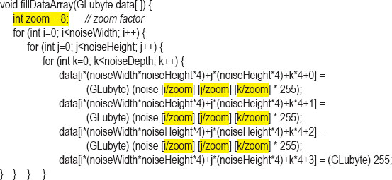
The “blockiness” within a given noise map can be smoothed by interpolating from each discrete grayscale color value to the next one. That is, for each small “block” within a given 3D texture, we set each texel color within the block by interpolating from its color to its neighboring blocks’ colors. The interpolation code is shown as follows in the function smoothNoise(), along with the modified fillDataArray() function. The resulting “smoothed” textures (for zooming factors 2, 4, 8, 16, 32, and 64—left to right, top to bottom) then follow in Figure 14.14. Note that the zoom factor is now a double, because we need the fractional component to determine the interpolated grayscale values for each texel.

The smoothNoise() function computes a grayscale value for each texel in the smoothed version of a given noise map by computing a weighted average of the eight grayscale values surrounding the texel in the corresponding original “blocky” noise map. That is, it averages the color values at the eight vertices of the small “block” the texel is in. The weights for each of these “neighbor” colors are based on the texel’s distance to each of its neighbors, normalized to the range [0..1].
Next, smoothed noise maps of various zooming factors are combined. A new noise map is created in which each of its texels is formed by another weighted average, this time based on the sum of the texels at the same location in each of the “smoothed” noise maps, with the zoom factor serving as the weight. The effect was dubbed “turbulence” by Perlin [PE85], although it is really more closely related to the harmonics produced by summing various waveforms. A new turbulence() function and a modified version of fillDataArray() that specifies a noise map that sums zoom levels 1 through 32 (the ones that are powers of two) are shown as follows, along with an image of a cube textured with the resulting noise map.
Figure 14.14
Smoothing of 3D textures, at various zooming levels.
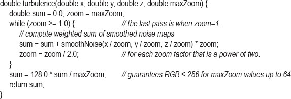
3D noise maps, such as the one shown in Figure 14.15, can be used for a wide variety of imaginative applications. In the next sections, we will use them to generate marble, wood, and clouds. The distribution of the noise can be adjusted by various combinations of zoom-in levels.
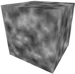
Figure 14.15
3D texture map with combined “turbulence” noise.
14.6NOISE APPLICATION – MARBLE
By modifying the noise map and adding Phong lighting with an appropriate ADS material as described previously in Figure 7.3, we can make the dragon model appear to be made of a marble-like stone.
We start by generating a striped pattern somewhat similar to the “stripes” example from earlier in this chapter—the new stripes differ from the previous ones, first because they are diagonal, and also because they are produced by a sine wave and therefore have blurry edges. We then use the noise map to perturb those lines, storing them as grayscale values. The changes to the fillDataArray() function are as follows:

The variable veinFrequency is used to adjust the number of stripes, turbSize adjusts the zoom factor used when generating the turbulence, and turbPower adjusts the amount of perturbation in the stripes (setting it to zero leaves the stripes unperturbed). Since the same sine wave value is used for all three (RGB) color components, the final color stored in the image data array is grayscale. Figure 14.16 shows the resulting texture map for various values of turbPower (0.0, 0.5, 1.0, and 1.5, left to right).
Since we expect marble to have a shiny appearance, we incorporate Phong shading to make a “marble” textured object look convincing. Program 14.5 summarizes the code for generating a marble dragon. The vertex and fragment shaders are the same as used for Phong shading, except that we also pass through the original vertex coordinates for use as 3D texture coordinates (as described earlier). The fragment shader combines the noise result with the lighting result using the technique described previously in Section 7.6.

Figure 14.16
Building 3D “marble” noise maps.
Program 14.5 Building a Marble Dragon
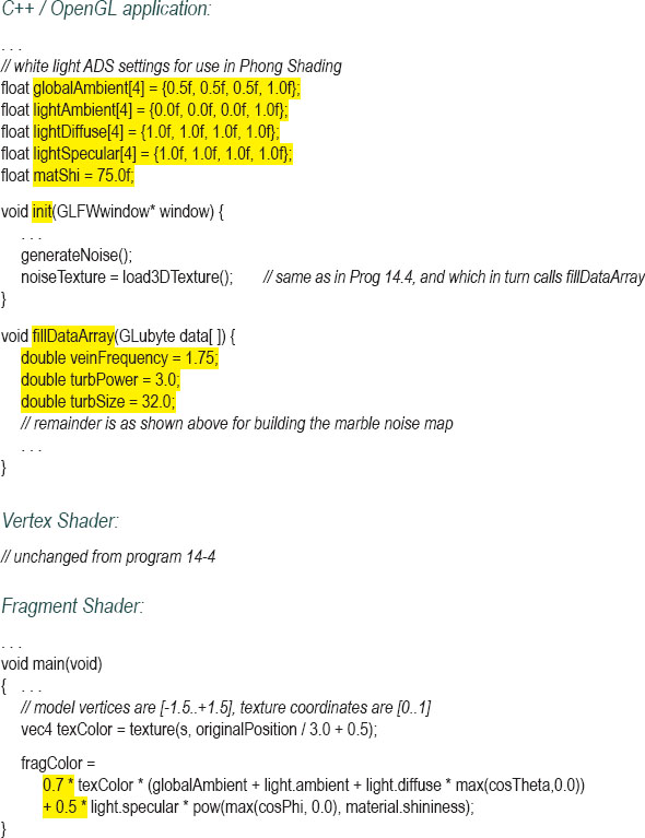
There are various ways of simulating different colors of marble (or other stones). One approach for changing the colors of the “veins” in the marble is by modifying the definition of the Color variable in the fillDataArray() function; for example, by increasing the green component:
float redPortion = 255.0f * (float)sineValue;
float greenPortion = 255.0f * (float)min(sineValue*1.5 - 0.25, 1.0);
float bluePortion = 255.0f * (float)sineValue;
We can also introduce ADS material values (i.e., specified in init()) to simulate completely different types of stone, such as “jade.”
Figure 14.17 shows four examples, the first three using the settings shown in Program 14.5, and the fourth incorporating the “jade” ADS material values shown earlier in Figure 7.3.
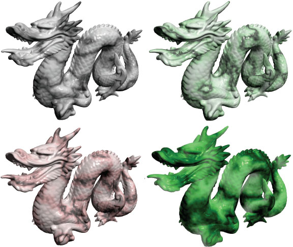
Figure 14.17
Dragon textured with 3D noise maps – three marble and one jade.
Creating a “wood” texture can be done in a similar way as was done in the previous “marble” example. Trees grow in rings, and it is these rings that produce the “grain” we see in objects made of wood. As trees grow, environmental stresses create variations in the rings, which we also see in the grain.
We start by building a procedural “rings” 3D texture map, similar to the “checkerboard” from earlier in this chapter. We then use a noise map to perturb those rings, inserting dark and light brown colors into the ring texture map. By adjusting the number of rings, and the degree to which we perturb the rings, we can simulate wood with various types of grain. Shades of brown can be made by combining similar amounts of red and green, with less blue. We then apply Phong shading with a low level of “shininess.”
We can generate rings encircling the Z-axis in our 3D texture map by modifying the fillDataArray() function, using trigonometry to specify values for X and Y that are equidistant from the Z axis. We use a sine wave to repeat this process cyclically, raising and lowering the red and green components equally based on this sine wave to produce the varying shades of brown. The variable sineValue holds the exact shade, which can be adjusted by slightly offsetting one or the other (in this case increasing the red by 80, and the green by 30). We can create more (or fewer) rings by adjusting the value of xyPeriod. The resulting texture is shown in Figure 14.18.
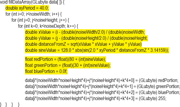
The wood rings in Figure 14.18 are a good start, but they don’t look very realistic—they are too perfect. To improve this, we use the noise map (more specifically, turbulence) to perturb the distanceFromZ variable so that the rings have slight variations. The computation is modified as follows:

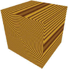
Figure 14.18
Creating rings for 3D wood texture.
Again, the variable turbPower adjusts how much turbulence is applied (setting it to 0.0 results in the unperturbed version shown in Figure 14.18), and maxZoom specifies the zoom value (32 in this example). Figure 14.19 shows the resulting wood textures for turbPower values 0.05, 1.0, and 2.0 (left to right).
We can now apply the 3D wood texture map to a model. The realism of the texture can be further enhanced by applying a rotation to the originalPosition vertex locations used for texture coordinates; this is because most items carved out of wood don’t perfectly align with the orientation of the rings. To accomplish this, we send an additional rotation matrix to the shaders for rotating the texture coordinates. We also add Phong shading, with appropriate wood-color ADS values, and a modest level of shininess. The complete additions and changes for creating a “wood dolphin” are shown in Program 14.6.

Figure 14.19
“Wood” 3D texture maps with rings perturbed by noise map.
Program 14.6 Creating a Wood Dolphin
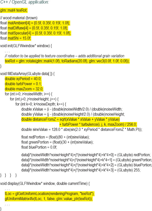
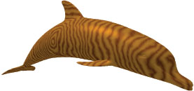
Figure 14.20
Dolphin textured with “wood” 3D noise map.
The resulting 3D textured wood dolphin is shown in Figure 14.20.
There is one additional detail in the fragment shader worth noting. Since we are rotating the model within the 3D texture, it is sometimes possible for this to cause the vertex positions to move beyond the required [0..1] range of texture coordinates as a result of the rotation. If this were to happen, we could adjust for this possibility by dividing the original vertex positions by a larger number (such as 4.0 rather than 2.0), and then adding a slightly larger number (such as 0.6) to center it in the texture space.
14.8NOISE APPLICATION – CLOUDS
The “turbulence” noise map built earlier in Figure 14.15 already looks a bit like clouds. Of course, it isn’t the right color, so we start by changing it from grayscale to an appropriate mix of light blue and white. A straightforward way of doing this is to assign a color with a maximum value of 1.0 for the blue component and varying (but equal) values between 0.0 and 1.0 for the red and green components, depending on the values in the noise map. The new fillDataArray() function follows:
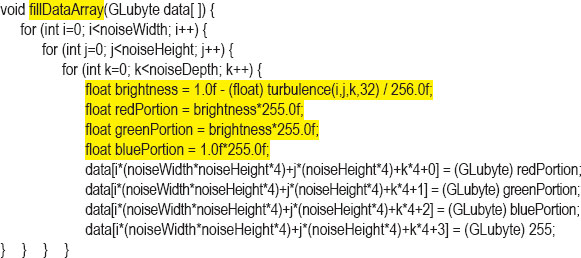
The resulting blue version of the noise map can now be used to texture a skydome. Recall that a skydome is a sphere or half-sphere that is textured, rendered with depth-testing disabled, and placed so that it surrounds the camera (similar to a skybox).
One way of building the skydome would be to texture it in the same way as we have for other 3D textures, using the vertex coordinates as texture coordinates. However, in this case, it turns out that using the skydome’s 2D texture coordinates instead produces patterns that look more like clouds, because the spherical distortion slightly stretches the texture map horizontally. We can grab a 2D slice from the noise map by setting the third dimension in the GLSL texture() call to a constant value. Assuming that the skydome’s texture coordinates have been sent to the OpenGL pipeline in a vertex attribute in the standard way, the following fragment shader textures it with a 2D slice of the noise map:
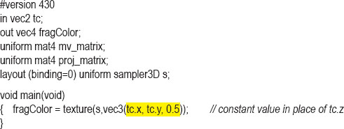
Figure 14.21
Skydome textured with misty clouds.
The resulting textured skydome is shown in Figure 14.21. Although the camera is usually placed inside the skydome, we have rendered it here with the camera outside, so that the effect on the dome itself can be seen. The current noise map leads to “misty-looking” clouds.
Although our misty clouds look nice, we would like to be able to shape them—that is, make them more or less hazy. One way of doing this is to modify the turbulence() function so that it uses an exponential, such as a logistic function,2 to make the clouds look more “distinct.” The modified turbulence() function is shown in Program 14.7, along with an associated logistic() function. The complete Program 14.7 also incorporates the smooth(), fillDataArray(), and generateNoise() functions described earlier.
Program 14.7 Cloud Texture Generation
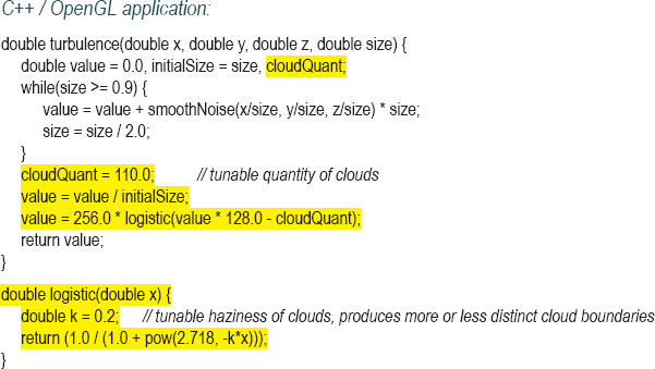
The logistic function causes the colors to tend more toward white or blue, rather than values in between, producing the visual effect of there being more distinct cloud boundaries. The variable cloudQuant adjusts the relative amount of white (versus blue) in the noise map, which in turn leads to more (or fewer) generated white regions (i.e., distinct clouds) when the logistic function is applied. The resulting skydome, now with more distinct cloud formations, is shown in Figure 14.22.
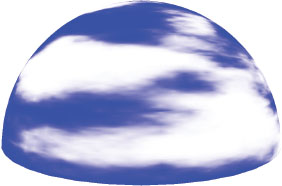
Figure 14.22
Skydome with exponential cloud texture.
Lastly, real clouds aren’t static. To enhance the realism of our clouds, we should animate them by (a) making them move or “drift” over time and (b) gradually changing their form as they drift.
One simple way of making the clouds “drift” is to slowly rotate the skydome. This isn’t a perfect solution, as real clouds tend to drift in a straight direction rather than rotating around the observer. However, if the rotation is slow and the clouds are simply for decorating a scene, the effect is likely to be adequate.
Having the clouds gradually change form as they drift may at first seem tricky. However, given the 3D noise map we have used to texture the clouds, there is actually a very simple and clever way of achieving the effect. Recall that although we constructed a 3D texture noise map for clouds, we have so far only used one “slice” of it, in conjunction with the skydome’s 2D texture coordinates (we set the “Z” coordinate of the texture lookup to a constant value). The rest of the 3D texture has so far gone unused.
Our trick will be to replace the texture lookup’s constant “Z” coordinate with a variable that changes gradually over time. That is, as we rotate the skydome, we gradually increment the depth variable, causing the texture lookup to use a different slice. Recall that when we built the 3D texture map, we applied smoothing to the color changes along all three axes. So, neighboring slices from the texture map are very similar, but slightly different. Thus, by gradually changing the “Z” value in the texture() call, the appearance of the clouds will gradually change.
The code changes to cause the clouds to slowly move and change over time are shown in Program 14.8.
Program 14.8 Animating the Cloud Texture
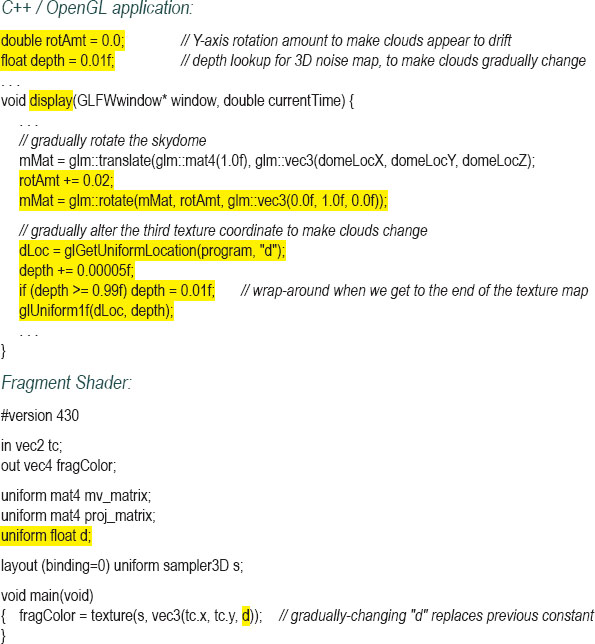
While we cannot show the effect of gradually changing drifting and animated clouds in a single still image, Figure 14.23 shows such changes in a series of snapshots of the 3D generated clouds as they drift across the skydome from right to left and slowly change shape while drifting.
Figure 14.23
3D clouds changing while drifting.
14.9NOISE APPLICATION – SPECIAL EFFECTS
Noise textures can be used for a variety of special effects. In fact, there are so many possible uses that its applicability is limited only by one’s imagination.
One very simple special effect that we will demonstrate here is a dissolve effect. This is where we make an object appear to gradually dissolve into small particles, until it eventually disappears. Given a 3D noise texture, this effect can be achieved with very little additional code.
To facilitate the dissolve effect, we introduce the GLSL discard command. This command is only legal in the fragment shader, and when executed, it causes the fragment shader to discard the current fragment (meaning not render it).
Our strategy is a simple one. In the C++/OpenGL application, we create a fine-grained noise texture map identical to the one shown back in Figure 14.12, and also a float variable counter that gradually increases over time. This variable is then sent down the shader pipeline in a uniform variable, and the noise map is also placed in a texture map with an associated sampler. The fragment shader then accesses the noise texture using the sampler—in this case we use the returned noise value to determine whether or not to discard the fragment. We do this by comparing the grayscale noise value against the counter, which serves as a sort of “threshold” value. Because the threshold is gradually changing over time, we can set it up so that gradually more and more fragments are discarded. The result is that the object appears to gradually dissolve. Program 14.9 shows the relevant code sections, which are added to the earth-rendered sphere from Program 6.1. The generated output is shown in Figure 14.24.
Program 14.9 Dissolve Effect Using discard Command
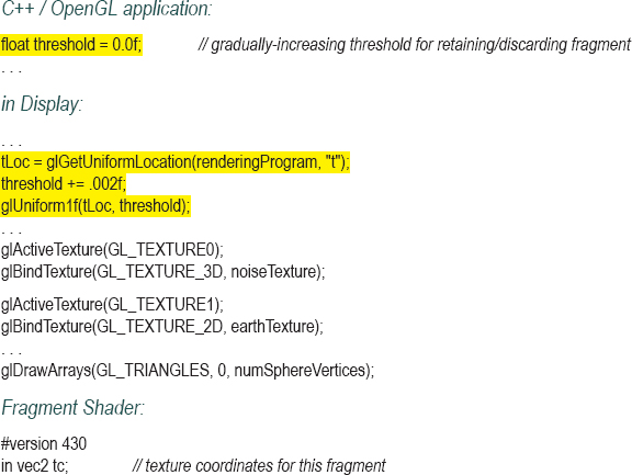
The discard command should, if possible, be used sparingly, because it can incur a performance penalty. This is because its presence makes it more difficult for OpenGL to optimize Z-buffer depth testing.
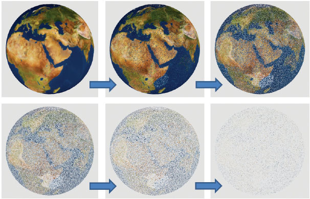
Figure 14.24
Dissolve effect with discard shader.
In this chapter, we used Perlin noise to generate clouds and to simulate both wood and a marble-like stone from which we rendered the dragon. People have found many other uses for Perlin noise. For example, it can be used to create fire and smoke [CC16, AF14], build realistic bump maps [GR05], and has been used to generate terrain in the video game Minecraft [PE11].
The noise maps generated in this chapter are based on procedures outlined by Lode Vandevenne [VA04]. There remain some deficiencies in our 3D cloud generation. The texture is not seamless, so at the 360° point there is a noticeable vertical line. (This is also why we started the depth variable in Program 14.8 at 0.01 rather than at 0.0—to avoid encountering the seam in the Z dimension of the noise map). Simple methods exist for removing the seams [AS04], if needed. Another issue is at the northern peak of the skydome where the spherical distortion in the skydome causes a pincushion effect.
The clouds we implemented in this chapter also fail to model some important aspects of real clouds, such as the way that they scatter the sun’s light. Real clouds also tend to be more white on the top and grayer at the bottom. Our clouds also don’t achieve a 3D “fluffy” look that many actual clouds have.
Similarly, more comprehensive models exist for generating fog, such as the one described by Kilgard and Fernando [KF03].
While perusing the OpenGL documentation, the reader might notice that GLSL includes some noise functions named noise1(), noise2(), noise3(), and noise4(), which are described as taking an input seed and producing Gaussian-like stochastic output. We didn’t use these functions in this chapter because, as of this writing, most vendors have not implemented them. For example, many NVIDIA cards currently return 0 for these functions, regardless of the input seed.
Exercises
14.1Modify Program 14.2 to gradually increase the alpha value of an object, causing it to gradually fade out and eventually disappear.
14.2Modify Program 14.3 to clip the torus along the horizontal, creating a circular “trough.”
14.3Modify Program 14.4 (the version including the modification in Figure 14.10 that produces a 3D cubed texture) so that it instead textures the Studio 522 dolphin. Then observe the results. Many people when first observing the result—such as that shown on the dragon, but also even on simpler objects—believe that there is some error in the program. Unexpected surface patterns can result from “carving” an object out of 3D textures, even in simple cases.
14.4The simple sine wave used to define the wood “rings” (shown in Figure 14.18) generate rings in which the light and dark areas are equal width. Experiment with modifications to the associated fillDataArray() function with the goal of making the dark rings narrower in width than the light rings. Then observe the effects on the resulting wood-textured object.
14.5(PROJECT) Incorporate the logistic function (from Program 14.7) into the marble dragon from Program 14.5, and experiment with the settings to create more distinct veins.
14.6Modify Program 14.9 to incorporate the zooming, smoothing, turbulence, and logistic steps described in prior sections. Observe the changes in the resulting dissolve effect.
References
[AF14] |
S. Abraham and D. Fussell, “Smoke Brush,” Proceedings of the Workshop on Non-Photorealistic Animation and Rendering (NPAR’14), 2014, accessed October 2018, https://www.cs.utexas.edu/~theshark/smokebrush.pdf |
[AS04] |
D. Astle, “Simple Clouds Part 1,” gamedev.net, 2004, accessed October 2018, http://www.gamedev.net/page/resources/_/technical/game-programming/simple-clouds-part-1-r2085 |
[CC16] |
A Fire Shader in GLSL for your WebGL Games (2016), Clockwork Chilli (blog), accessed October 2018, http://clockworkchilli.com/blog/8_a_fire_shader_in_glsl_for_your_webgl_games |
[GR05] |
S. Green, “Implementing Improved Perlin Noise,” GPU Gems 2, NVIDIA, 2005, accessed October 2018, https://developer.nvidia.com/gpugems/GPUGems2/gpugems2_chapter26.html |
[JA12] |
A. Jacobson, “Cheap Tricks for OpenGL Transparency,” 2012, accessed October 2018, http://www.alecjacobson.com/weblog/?p=2750 |
M. Kilgard and R. Fernando, “Advanced Topics,” The Cg Tutorial (Addison-Wesley, 2003), accessed October 2018, http://http.developer.nvidia.com/CgTutorial/cg_tutorial_chapter09.html | |
[LU16] |
F. Luna, Introduction to 3D Game Programming with DirectX 12, 2nd ed. (Mercury Learning, 2016). |
[PE11] |
M. Persson, “Terrain Generation, Part 1,” The Word of Notch (blog), Mar 9, 2011, accessed October 2018, http://notch.tumblr.com/post/3746989361/terrain-generation-part-1 |
[PE85] |
K. Perlin, “An Image Synthesizer,” SIGGRAPH ʻ85 Proceedings of the 12th annual conference on computer graphics and interactive techniques (1985). |
[VA04] |
L. Vandevenne, “Texture Generation Using Random Noise,” Lode’s Computer Graphics Tutorial, 2004, accessed October 2018, http://lodev.org/cgtutor/randomnoise.html |
1The Technical Achievement Award, given by the Academy of Motion Picture Arts and Sciences.
2A “logistic” (or “sigmoid”) function has an S-shaped curve with asymptotes on both ends. Common examples are hyperbolic tangent and f(x) = 1/(1+e-x). They are also sometimes called “squashing” functions.