Chapter 2. Genomics in a Nutshell: A Primer for Newcomers to the Field
Now that we’ve given you the broad context of the book in Chapter 1, it’s time to dive into the more specific scientific context of genomics. In this chapter, we run through a brief primer on key biological concepts and related practical information that you need to know in order to benefit fully from working through the exercises in this book. We review the fundamentals of genetics and build up to a definition of genomics that will frame the scientific scope of this book. With that frame in place, we then review the main types of genomics variation, with a focus on how they manifest in the genome. Finally, we go over the key processes, tools, and file formats involved in generating and processing high-throughput sequencing data for genomic analysis.
Depending on your background, this might serve as a quick refresher, or it might be your first introduction to many of these topics. The first couple of sections are aimed at readers who have not had much formal training in biology, genetics, and related life sciences. If you are a life-sciences student or professional, feel free to skim through until you encounter something that you don’t already know. In later sections, we progressively introduce more genomics-specific concepts and tools that should be useful to all but the most seasoned practitioners.
Introduction to Genomics
So what is genomics? The short answer, “it’s the science of genomes,” doesn’t really help if you don’t already know what a genome is and why it matters. So before we get into the gory details of “how to do genomics,” let’s take a step back and make sure we all agree on what we mean by genomics. First, let’s go over the fundamental concepts involved, including the basics of what a gene is and how it relates to DNA. Then, we progressively deepen our exploration to cover key types of data and analyses within the specific defined scope. Keep in mind that this will not be an exhaustive compilation of all things that could possibly be grouped under the term of genomics, given that (a) this is not meant to be a scientific textbook, and (b) the field is still evolving very rapidly, with so many exciting new methodologies and technologies being actively developed that it would be premature to attempt to codify them in a book like this one.
The Gene as a Discrete Unit of Inheritance (Sort Of)
Let’s start at the historical beginning—the gene. It’s a term that is almost universally recognized but not necessarily well understood, so it’s worth going into its origins and unrolling its evolution (so to speak).
The earliest mention of a gene was based on concepts formulated by key 19th-century thinkers such as Charles “Origin of Species” Darwin and Gregor “Pea Enthusiast” Mendel, at a time when the advent of molecular biology was still well more than a century away. They needed a way to explain the patterns of partial and combinatorial trait inheritance that they had observed in various organisms, so they postulated the existence of microscopic indivisible particles that are transmitted from parents to progeny and constitute the determinants of physical traits. These hypothetical particles were eventually dubbed genes by Wilhelm Johannsen in the early 20th century.
A fistful of decades later, Rosalind Franklin, Francis Crick, and James Watson elucidated the now famous double-helix structure of DNA: two complementary strands, each formed by a backbone of repeated units of a molecule called deoxyribose (the D in DNA), which carry the actual information content in the form of another type of molecule called nucleic acids (the NA in DNA). The four nucleic acids in DNA, more generally called bases, are famously referred to by their initials A, C, G, and T, which stand for adenine, cytosine, guanine, and thymine, respectively. The reason DNA works as a double helix is that the molecular structure of the bases makes the two strands pair up: if you put an A base across from a T base, their shapes match up, and they attract each other like magnets. The same thing happens with G and C, except they attract each other even more strongly than A and T, because G and C form three bonds, whereas A and T form only two bonds. The implications of this simple biochemical complementarity are enormous; sadly, we don’t have time to go into all of that, but we leave you with Crick and Watson’s classic understatement in their original paper on the structure of DNA:
It has not escaped our notice that the specific pairing we have postulated immediately suggests a possible copying mechanism for the genetic material.
Combine the concept of genes and the reality of DNA, and it turns out that the units we call genes correspond to fairly short regions that we delineate within immensely long strings of DNA. Those long strings of DNA are what make up our chromosomes, which most people recognize as the X-shaped squiggles in their high school biology textbooks. As illustrated in Figure 2-1, that X shape is a condensed form of the chromosome in which the DNA is tightly wound.
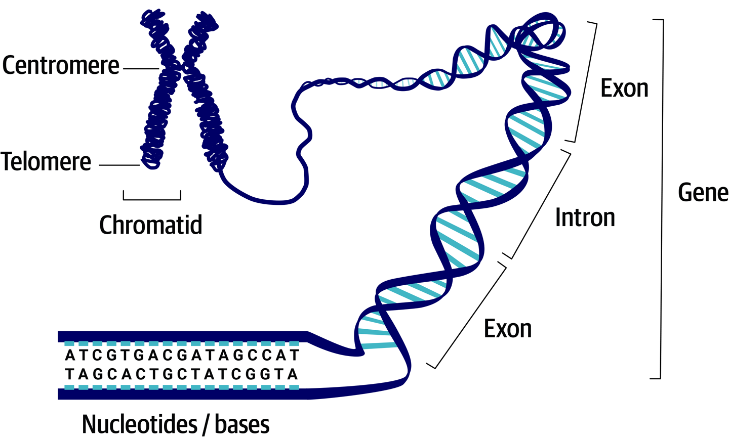
Figure 2-1. The chromosome (shown here in the form of two sister chromatids, each composed of one incredibly long molecule of double-stranded DNA) on which we delineate genes composed of exons and introns.
Like many other living creatures, human beings are diploid, which means that you have two copies of each chromosome: one inherited from each biological parent. As a result, you have two copies of every gene that is present on both chromosomes, which amounts to most of your genes. In a few cases, some genes might be present on one chromosome and absent from the other, but we won’t go into those here. For a given gene, your two copies are called alleles, and they’re typically not strictly identical in sequence to each other. If you produce a biological child, you pass on to them one chromosome from each of your 23 pairs and, accordingly, one of your two alleles for every gene. This concept of allele will be very important in the context of variant discovery, in which it will apply to individual variants instead of the overall gene.
Note
Although the X-shaped form is their most common representation in popular media, our chromosomes don’t spend much time looking like that. Most of the time they are in a rod-shaped form called a chromatid. When the single chromatid is copied ahead of a cell division event, the two identical chromatids are connected by a central region called the centromere, resulting in the popular X shape. Be careful not to confuse sister chromatids, which belong to the same chromosome, with the chromosome copies that you inherit from each biological parent.
If we look more closely at the span of a region of DNA that is defined as a gene, we see that the gene itself is split into smaller regions called exons and introns. When a particular gene is called into action, the exons are the parts that are going to contribute to its functionality, whereas the introns will be ignored. If you have a difficult time not mixing them up, try to remember that exons are the exciting parts, and introns are the bits in between.
All this suggests that genes are not really like the discrete particles that our forerunners originally envisioned. If anything, chromosomes are closer to being discrete units of inheritance, at least in the physical sense, given that each corresponds to an unbroken molecule of DNA. Indeed, many traits caused by different genes are inherited together because when you inherit one copy of a chromosome, there is a physical linkage between all the genes that it carries. Then again, the reality of chromosomal inheritance is more complex than you might expect. Just before the cell division that produces eggs and sperm cells, the parental chromosome copies pair up and swap segments with each other in a process called chromosomal recombination, which shuffles the combinations of physically linked traits that will be transmitted to the progeny. Heads-up: biology is messy that way.
Now that we have a handle on the basic terminology and mechanisms of genetic inheritance, let’s look into what genes actually do.
The Central Dogma of Biology: DNA to RNA to Protein
This central dogma is the next level in our understanding of what genes are and how they work. The idea is that the “blueprint” information encoded in genes in the form of DNA is transcribed into a closely related intermediate form called ribonucleic acid, or RNA, which our cells then use as a guide to string together amino acids into proteins. The main differences between DNA and RNA are that RNA has one different nucleotide (uracil instead of thymine, but it still sticks to adenine) and it’s a lot less stable biochemically. You can think of DNA as the master blueprint, and RNA as working copies of sections of the master blueprint. Those working copies are what the cell will use to build proteins. These proteins range in function from structural components (e.g., muscle fiber) to metabolic agents (e.g., digestive enzymes) and ultimately act as both the bricks and bricklayers of our bodies.
The process as a whole is called gene expression (see Figure 2-2). It makes a ton of sense and explains a lot—yet this is not the complete picture. As a description of a gene expression process, it would have been true, but for several decades the theory went on to state that this flow of information was strictly unidirectional and comprehensive. Yep, you guessed it: just like the gene concept, this turned out to be somewhat wrong. We have since discovered various ways in which life violates this long-held dogma: for example, through DNA-to-RNA-only as well as RNA-only pathways, which modify gene expression in a variety of fun and baffling ways. Pathways also exist that lead to protein synthesis without the guidance of an RNA template, called nonribosomal protein synthesis, which some bacteria use to produce small molecules that play various roles such as intercellular signaling and microbial warfare (i.e., antibiotics). Again, keep in mind that reality is more complicated than the cartoon version, though the cartoon version is still useful to convey the most common relationship between the major players: DNA, RNA, amino acids, and proteins.

Figure 2-2. The central dogma of biology: DNA leads to RNA; RNA leads to amino acids; amino acids lead to protein.
So how does that relationship work in practice? How do you go from DNA sequence to the amino acids that make up the proteins? First, the transcription of DNA to RNA uses a neat biochemical trick: as we mentioned earlier, the nucleotides are complementary to one another—A sticks to T/U, and C sticks to G—thus, if you have a string of DNA that reads TACTTGATC, the cell can generate a “messenger” RNA string by placing the appropriate (i.e., sticky) RNA base opposite each DNA base, to produce AUGAACUAG. Then, it’s time for the genetic code to come into play: each set of three letters constitutes a codon that corresponds to an amino acid, as shown in Figure 2-3. A cellular tool called a ribosome reads each codon and lines up the corresponding amino acid to add it to the chain, which will eventually become a protein. Our minimalist example sequence therefore codes for a very short amino acid chain: just methionine (AUG) followed by asparagine (AAC). The third codon (UAG) simply signals the ribosome to stop extending the chain.
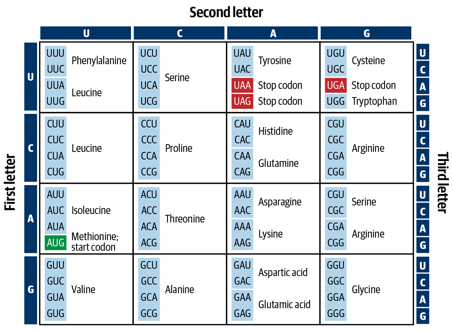
Figure 2-3. The genetic code connects three-letter codons in a messenger RNA sequence to specific amino acids.
We could explain a lot more about how all of this works, as it’s really quite fascinating, so we encourage you to look it up to learn more. For now, what we want to emphasize is the dependence of this mechanism on the DNA sequence: changing the sequence of the DNA can lead to changes in the amino acid sequence of the protein, which can affect its function. So let’s talk about genetic changes.
The Origins and Consequences of DNA Mutations
DNA is pretty stable, but sometimes it breaks (e.g., because of exposure to radiation or chemicals) and needs to be repaired. The enzymes that are responsible for repairing these breaks occasionally make mistakes and incorporate the wrong nucleic acid (e.g., a T instead of an A). The same applies for the enzymes responsible for making copies of DNA during cell division; they make mistakes, and sometimes those mistakes persist and are transmitted to progeny. Between these and other mechanisms of mutation that we won’t go into here, the DNA that each generation inherits from their parents diverges a little more over time. The overwhelming majority of these mutations do not have any functional effects, in part because some redundancy is present in the genetic code: you can change some letters without changing the meaning of the “word” that they spell out.
However, as illustrated in Figure 2-4, some mutations do have effects that cause an alteration in gene function, gene expression, or related processes. These effects might be positive; for example, improving the efficiency of an enzyme that degrades toxins and thereby protects your body from damage. Others will be negative; for example, reducing that same enzyme’s efficiency. Some changes might have dual effects depending on context; for example, one well-known example of a mutation contributes to sickle-cell disease but protects against malaria. Finally, some changes can have functional effects that are not obviously associated with a direct positive or negative outcome, like hair or eye color.
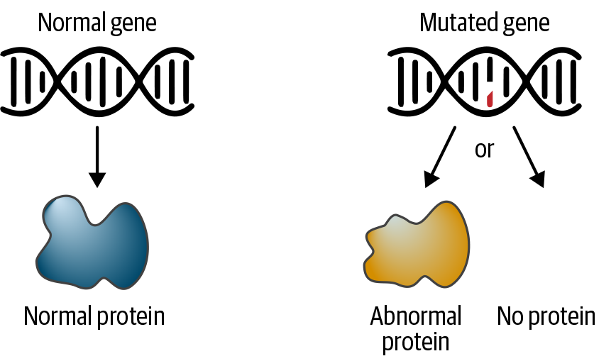
Figure 2-4. A mutation in the DNA sequence can cause the gene’s protein product to function abnormally or disable its production entirely.
Again, this topic is vastly more complex than we show here; our goal is mainly to illustrate why we care so much about determining the exact sequence of people’s genomes.
Genomics as an Inventory of Variation in and Among Genomes
Now that we’ve gone over the fundamentals, we can step back and take another stab at defining genomics. Let’s say the relationship between DNA and genes can be roughly summarized as “genes are made of DNA, but your DNA overall comprises both genes and nongenes.” This is an awkward formulation, so we’re going to use the term genome to refer to “your DNA overall.” But if genome means “all of your DNA including (but not limited to) your genes,” what should genomics encompass as “the science of genomes”?
The US-based NHGRI website declares:
Genetics refers to the study of genes and the way that certain traits or conditions are passed down from one generation to another. Genomics describes the study of all of a person’s genes (the genome).
The problem with that definition (beyond the rather cavalier omission of “all the DNA that is not part of genes”) is that the minute you begin looking for something specific in the genome, it becomes a question of genetics. For example, out of all the human genome, what are the genes involved in the development of type 2 diabetes? Is that genomics or genetics? Technically you need to look at all of the genes first in order to narrow down your search to the genes that will be meaningful to your research. So the “some genes” versus “all the genes” distinction is a rather fuzzy one that is not entirely helpful, at least not in the context of our book. We therefore define genomics more narrowly as the discipline tasked with identifying the contents of genomes, whether at the level of individuals, families, or populations. In this view, the goal of genomics is to produce the information that feeds into the downstream genetic analyses that will ultimately yield biological insights.
This definition includes the process of identifying which genomic contents are specific to individuals, which are shared among individuals and populations, and which are different among individuals and populations. A few related disciplines complement this subdivision, including transcriptomics, which is the study of gene expression at the genome scale. The term genomics is sometimes used as a catch-all for these disciplines, though it has now become more common to use the more generic term omics for that purpose. We won’t go into the details of those either, except to note the points of connection when the opportunity arises.
Note
We can use genome in the individual sense (as in “my personal genome”) and in the collective sense (as in “the human genome”).
The Challenge of Genomic Scale, by the Numbers
Approximately three billion base pairs are in a human genome, or three gigabases (GB), representing an enormous amount of biochemically encoded informational content. The technology we use to decipher this content generates hundreds of millions of very short sequences for a single genome. Specifically, about 40 million sequences of ~200 bases, which amounts to a 100 GB file per genome. If you do the math, you’ll realize that this dataset is redundant by a factor of 30 times! This is intentional, because the data is full of errors—some random, some systematic—so we need the redundancy to have enough confidence in our findings. Within that mass of data that is redundant but full of errors, we need to identify the four to five million small differences that are real (relative to a reference framework, which we discuss in the next section). That information can then be used to perform the genetic analysis that will determine which differences actually matter to a particular research question. Oh, and that’s for just one person; but we might want to apply this to cohorts of hundreds, thousands, tens of thousands of people, or more. (Spoiler alert: definitely more.)
Given the scale involved, we’re going to need some very robust procedures for analyzing this data. But before we begin tackling the computational methods, let’s take a deeper look at the topic of genomic variation to define more precisely what we’re going to be looking for.
Genomic Variation
Genomic variation can take multiple forms and can arise at different times in the life cycles of organisms and populations. In this section, we review the way variants are described and classified. We begin by discussing the concept of a reference genome that is used as a common framework for cataloging variants. Then, we go over the three major classes of variants that are defined on the basis of the physical change that is involved: short sequence variants, copy-number variants, and structural variants. Finally, we discuss the difference between germline variants and somatic alterations, and where de novo mutations fit into the picture.
The Reference Genome as Common Framework
When it comes to comparing variation between genomes, whether it’s between cells or tissues of the same individual, or between individuals, families, or entire populations, almost all analyses rely on using a common genome reference sequence.
Why? Let’s look at a similar, if simpler problem. We have three modern-day sentences that we know evolved from a common ancestor:
-
The quick brown fax jumped over the lazy doge.
-
The quick _ fox jumped over their lazy doge.
-
The quick brown fox jumps over the lazy brown dog.
We’d like to inventory their differences in a way that is not biased toward any single one of them, and is robust to the possibility of adding new mutant sentences as we encounter them. So we create a synthetic hybrid that encapsulates what they have most in common, yielding this:
The quick brown fox jumped over the lazy doge.
We can use this as a common reference coordinate system against which we can plot what is different (if not necessarily unique) in each mutant:
-
Fourth word, o → a substitution; ninth word, deleted e
-
Third word deleted; seventh word, added ir; ninth word, added e
-
Fifth word ed → s substitution; duplication of the third word located after the eighth word
It’s obviously not a perfect method, and what it gives us is not the true ancestral sentence: we suspect that’s not how dog was originally spelled, and we’re unsure of the original tense (jumps versus jumped). But it enables us to distinguish what is commonly observed in the population we have access to from what is divergent.
The more sentences we can involve in the initial formulation of this reference and the more representative the sampling, the more appropriate it will be for describing the variations we encounter in the future.
Similarly, we use a reference genome in order to chart sequence variation in individuals against a common standard rather than attempting to chart differences between genome sequences relative to one another. That enables us to identify what subset of variations in sequence are commonly observed versus unique to particular samples, individuals, or populations.
So whose genome do we use as a common framework? In the simplest case, any individual genome can be used as a reference genome. However, our analysis will produce better results if we can use a reference genome that is representative of the widest group of individuals that we might want to study.
That leads to a complicated problem: for our reference to be representative of many individuals, we need to evaluate the most commonly observed sequence across available individual genomes, which we call a haplotype, for each segment of the genome reference. Then, we can use that information to compose a synthetic hybrid sequence. The result is a sequence that is never actually observed wholesale in any particular individual genome.
Researchers are trying to address these limitations using more advanced representations of genomes, such as graphs for which nodes represent different possible sequences, and edges between them allow you to trace a given genome. However, for the purposes of our analysis presented in this book, we use a high-quality reference genome derived from the efforts of the scientific community starting with the Human Genome Project (HGP).
It’s important to understand that the effectiveness of the common reference is limited by the diversity of the original samples used in its development. When the HGP was declared complete in 2003, the genome sequence that the HGP consortium published was, in fact, a synthetic reference based on a very small number of people, all from European background. This limited its effectiveness as a reference for non-European populations because, as we learned later, some of these populations have substantial enough differences that cannot be adequately mapped back to the original Euro-centric reference.
Successive “versions” of the human genome reference, commonly called assemblies or builds, have been published since then. In addition to delivering higher quality through purely technological advances, these updates to the common genome reference have also increased its representativeness by including more data from historically underrepresented populations. It is worth emphasizing that these efforts to compensate for historical bias in the selection of participants in genomic studies are very necessary. Indeed, lack of representation in research data leads to real inequalities in clinical outcomes because it affects our ability to identify meaningful variation in an individual’s genome sequence if that person belongs to an underrepresented population.
In humans, the most significant improvements to date have been made in the representation of so-called alternate haplotypes, regions that are sometimes dramatically different in different populations. The latest build of the human reference genome, officially named GRCh38 (for Genome Research Consortium human build 38) but commonly nicknamed Hg38 (for human genome build 38), greatly expanded the repertoire of alternate (ALT) contigs representing the alternate haplotypes. These have a significant impact on our power to detect and analyze genomic variation that is specific to populations carrying alternate haplotypes.
As a final plot twist, note that all current standard reference genome sequences are haploid, meaning they represent only one copy of each chromosome (or contig). The most immediate consequence is that in diploid organisms such as humans, which have two copies of each autosome (i.e., any chromosome that is not a sex chromosome, X or Y), the choice of standard representation of sites that are most often observed in heterozygous state (manifesting two different alleles; e.g., A/T) is largely arbitrary. This is obviously even worse in polyploid organisms, such as many plants including wheat and strawberries, which have higher numbers of chromosome copies. Although it is possible to represent reference genomes using graph-based representations, which would address this problem, few genome analysis tools are able to handle such representations at this time, and it will likely take years before graph-based genomes gain traction in the field.
Physical Classification of Variants
Now that we have a framework for describing variation, let’s talk about the kinds of variation we’ll be considering. We distinguish three major classes of variants based on the physical change they represent, which are illustrated in Figure 2-5. Short sequence variants (single-base changes and small insertions or deletions) are small changes in DNA sequence compared to a reference genome; copy-number variants are relative changes in the amount of a particular fragment of DNA; and structural variants are changes in the location or orientation of a particular fragment of DNA compared to a reference genome.
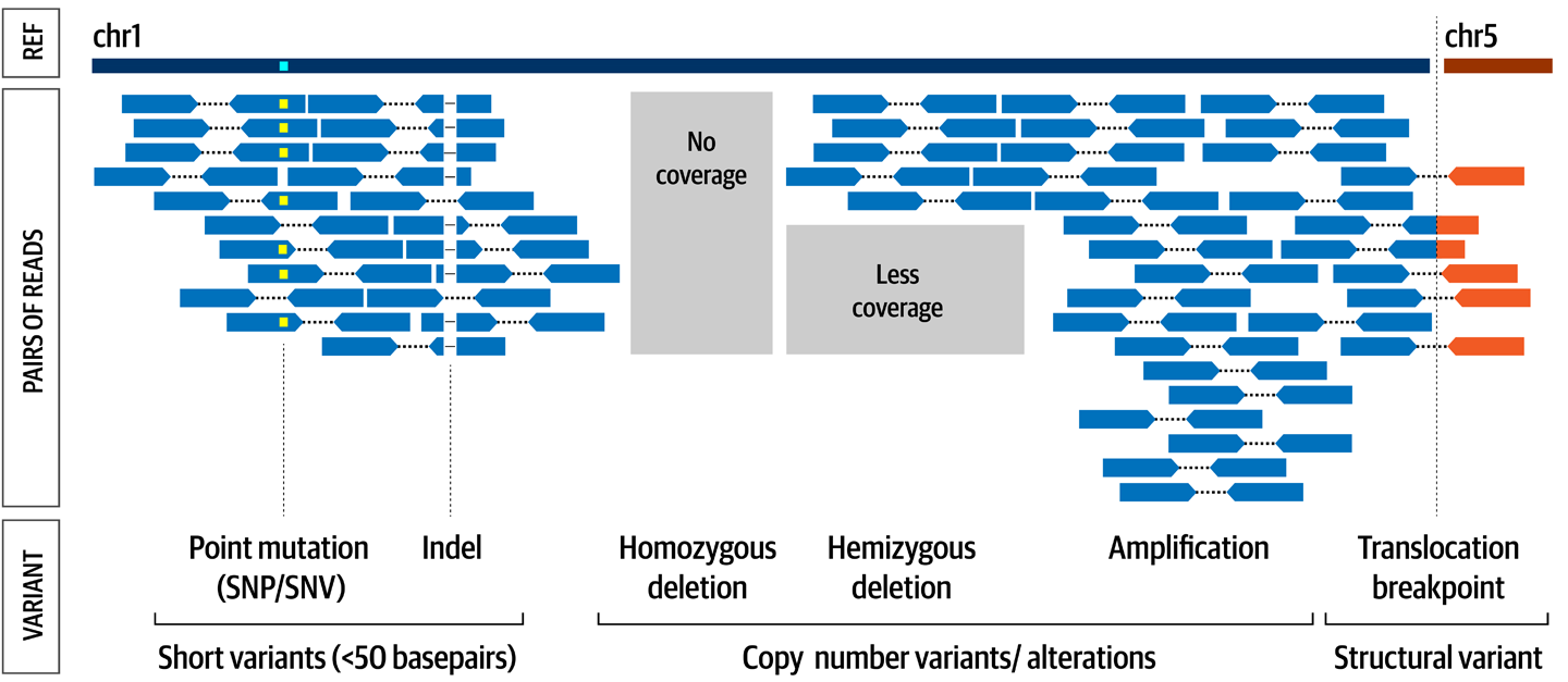
Figure 2-5. The major types of variant classified by physical changes to the DNA.
Single-nucleotide variants
Earlier, we examined the hybrid sentence: “The quick brown fox jumped over the lazy doge.” Within the list of three sentences, the first sentence used fax instead of fox. Here we might say there was a single-letter substitution in the word fox, where the o was substituted with an a because the “reference” says fox.
When we apply this to DNA sequence—for example, when we encounter a G nucleotide instead of the A we expect based on the reference—we’ll call it a single-nucleotide variant (Figure 2-6). Some variation exists in the exact terminology used to refer to these variants, and appropriately enough, the difference is a single-letter substitution: depending on context, we’ll call them either single-nucleotide polymorphism (SNP; pronounced “snip”), which is most appropriate in population genetics, or single-nucleotide variant (SNV; usually spelled out but sometimes pronounced “sniv”), which is more general in meaning yet is mostly used in cancer genomics.
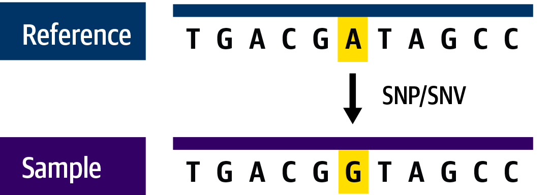
Figure 2-6. A single-nucleotide variant.
SNVs are the most common type of variation encountered in nature because the various mechanisms that cause them are fairly commonplace and their consequences are often minimal. Biological functions tend to be robust to such small changes because, as we saw earlier in our overview, the genetic code has multiple codons that code for the same amino acid, so single base changes don’t always lead to changes in the protein.
Insertions and deletions
In the second sentence of our example, “The quick _ fox jumps over their lazy doge,” we see the two primary types of small insertions and deletions: we’ve lost the word brown, and one instance of the has become their through the insertion of two letters. We also have one complex substitution in the replacement of jumped by jumps, which is interesting because without additional information we can’t say whether the change happened in a single event, ed becoming s, or whether the ed was lost first and the s was tacked on later. Or, the original ancestor of both jumped and jumps could have been jump, and both forms evolved later through independent insertions! That latter scenario seems more likely because it involves a simpler chain of events, but we can’t know for sure without seeing more data.
Applied to DNA sequence, indels are insertions or deletions of one or more bases compared to the reference sequence, as shown in Figure 2-7. Interestingly, multiple studies have reported that insertions occur more commonly than deletions (at least in humans). This observation has not been fully explained but could be related to naturally occurring mobile genetic elements, a kind of molecular parasite that is fascinating but sadly out of scope for this book.

Figure 2-7. Indels can be insertions (left) or deletions (right).
Note
The term indel is a portmanteau created by combining insertion and deletion.
Most indels observed in nature are fairly short, measuring less than 10 bases in length, but there is no maximum length of sequence than can be inserted or deleted. In practice, indels longer than a few hundred bases are generally classified as copy-number or structural variants, which we discuss next. Compared to single-nucleotide changes, indels are more likely to disrupt biological function, because they are more likely to cause phase shifts, where adding or removing bases shifts the three-letter reading frame used by the ribosome to read the codons. This can completely change the meaning of the sequence downstream of the indel. They can also cause protein folding changes when inserted into coding regions, for example.
Copy-number variants
With copy-number variation (Figure 2-8), we’re moving into a more complex territory because the game is no longer just a matter of playing “spot the difference.” Previously, the question was “What do I see at this location?” Now it shifts to “How many copies do I see of any given region?” For example, the third sentence in our evolved text example, “The quick brown fox jumps over the lazy brown dog” has two copies of the word brown.

Figure 2-8. Example of copy-number variant caused by a duplication.
In the biological context, if you imagine that each word is a gene that produces a protein, this means that we could produce twice as much “Brown” protein from this sentence’s DNA compared to the other two. That could be a good thing if the protein in question has, for instance, a protective effect against exposure to dangerous chemicals. But it could also be a bad thing if the amount of that protein present in the cell affects the production of another protein: increasing one could upset the balance of the other and cause a deleterious chain reaction that disrupts cellular processes.
Another case is the alteration of allelic ratio, the balance between two forms of the same gene. Imagine that you inherited a defective copy of a particular gene, which is supposed to repair damaged DNA, from your father, but it’s OK because you inherited a functional copy from your mother. That single functional copy is sufficient to protect you, because it makes enough protein to repair any damage to your DNA. Great. Now imagine that you have a for-now benign tumor in which one part suffers a copy-number event: it loses the functional copy from your mom, and now all you have is your dad’s broken copy, which is unable to produce the DNA repair protein. Those cells are no longer able to repair any DNA breaks (which can happen randomly) and begin to accumulate mutations. Eventually, that part of the tumor starts proliferating and becomes cancerous. Not so great.
These are called dosage effects and illustrate the biological complexity of genetic pathways that regulate cell metabolism and health. The DNA copy number can affect biological function in other ways, and in all cases the degree of severity of the effects depends on a lot of factors.
As an example, trisomies are genetic disorders in which patients have an extra copy of an entire chromosome. The most well-known is Down syndrome, which is caused by an extra copy of chromosome 21. It is associated with multiple intellectual and physical disabilities, but the people who carry them can live healthy and productive lives if they are supported appropriately. Trisomies affecting sex chromosomes (X and Y) tend to have fewer negative consequences; for example, most individuals with triple X syndrome experience no medical issues as a result. In contrast, several trisomies affecting other chromosomes are tragically incompatible with life and always result in either miscarriage or early infant death.
Structural variants
This last class of variants is a superset that includes copy-number variants and large indels in addition to various copy-neutral structural alterations such as translocations and inversions, as shown in Figure 2-9.
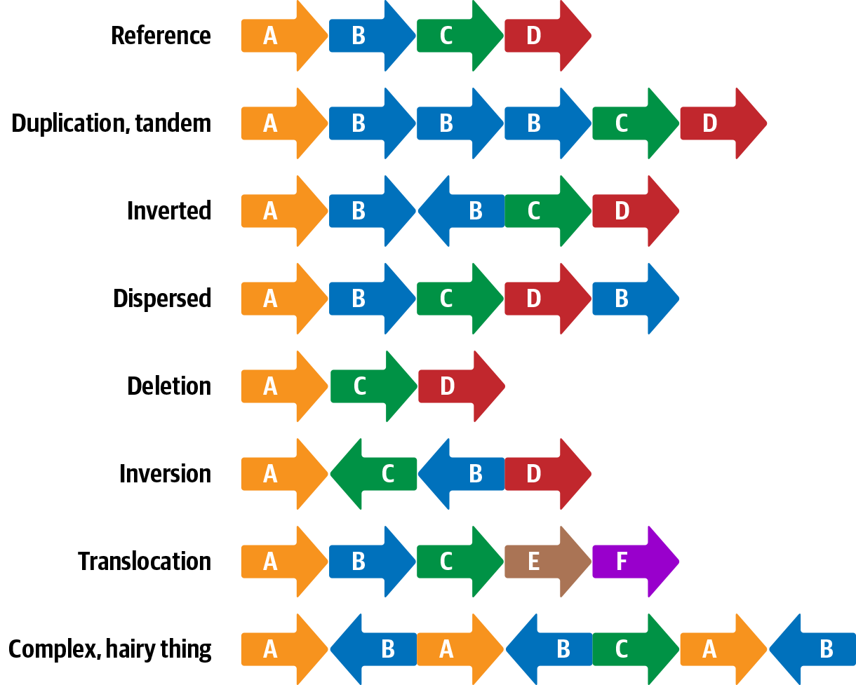
Figure 2-9. Examples of structural variants.
As you can see from the examples in Figure 2-9, structural variants can be rather complex because they cover a range of physical transformations of the genetic material. Some can span large distances, even affecting multiple chromosomes in some cases. We won’t cover structural variation in this book because this is still an area of very active development and the relevant methods are far from settled.
Germline Variants Versus Somatic Alterations
The fundamental biological distinction between germline variants and somatic alterations has major consequences for the way we approach variant discovery, depending on the specific purpose of the analysis. Wrapping your head around this can be a bit tricky because it’s tied to concepts of inheritance and embryo development. Let’s start from the definitions of the terms germline and somatic.
Germline
The term germline is a combination of two related aspects of biological inheritance. The germ part refers to the concept of germination of a seed, and doesn’t have anything to do directly with microbes, although it’s the same idea that causes us to call microbes germs. The line part refers to the fact that all cells that eventually turn into either eggs or sperm cells come from a single cell line, a population of cells with a common ancestor that get differentiated early in the development of the embryo.
In fact, the term germline is often used to refer to that entire population of cells as the germline of an individual. So in principle, your germline variants are variants that were present in your biological parents’ germline cells, typically the egg and/or sperm cell that produced you, before fertilization happened. As a result, your germline variants are expected to be present in every cell in your body. In practice, variants that arise very shortly after fertilization will be difficult or impossible to distinguish from germline variants.
Researchers are interested in germline variants for a variety of reasons: diagnosing diseases with a genetic component, predicting risk of developing disorders, understanding the origin of physical traits, mapping the origins and evolution of human populations—and that’s just on the human side! Germline variation within populations of organisms is also of great interest in agriculture, livestock improvement, ecological research, and even epidemiological monitoring of microbial pathogens.
Somatic
The term somatic is derived from the Greek word soma, meaning body. It’s used as an exclusionary term to refer to all cells that are not part of the germline, as illustrated in Figure 2-10. Somatic alterations are produced by mutation events in individual cells during the course of your life (including during embryo development, prior to birth), and are present only in subsets of cells in your body.
These mutations can be caused by a variety of factors, from genetic predispositions to environmental exposure to mutagens such as radiation, cigarette smoke, and other harmful chemicals. A great many of these mutations arise in your body but stay confined to one or a few cells and cause no noticeable effects. In some cases, the mutations can cause domino effects within the affected cells, damaging their ability to regulate growth and causing the formation of a cell tumor. Many tumors are thankfully benign; however, some become malignant and cause negative chain reactions, fueling the occurrence of many additional somatic mutations and resulting in metabolic diseases, which we ultimately group under the label of cancer.
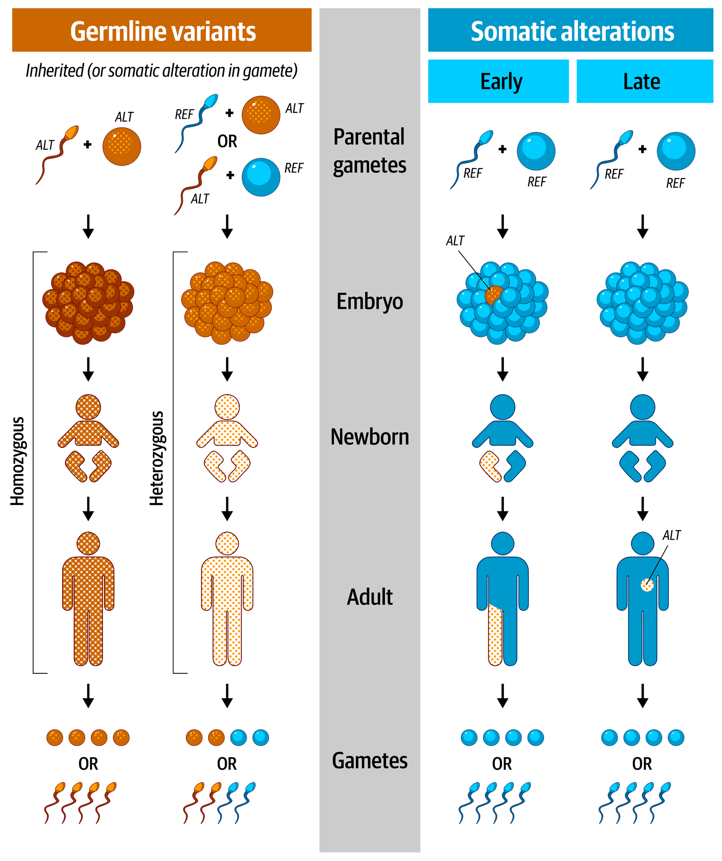
Figure 2-10. Germline variants are present in all cells of the body (left) while somatic alterations are present only in a subset of cells (right).
That being said, even though cancer research is one of the major applications of somatic variation analysis, the effects of somatic variation are not limited to tumor growth and cancer. They also include various developmental disorders such as Down syndrome, which, as we alluded to earlier, is caused by an erroneous duplication of chromosome 21; in other words, a form of CNV. Although Down syndrome can be inherited through the germline, it is most commonly observed as the result of an abnormal cell division event that occurs early on during the development of the embryo. Most of the time this happens so early that virtually all of the individual’s cells are affected.
This is where the line between germline variation and somatic alteration becomes a bit blurry. As we’ve just discussed, you can have a child born with a variant that arose very early on during their development. As far as its origin is concerned, it’s a somatic alteration; however, in the analysis of your child’s genome, it will manifest as a germline variant because it’s present in all of their cells. Along similar lines, you can get somatic mutations within your germline cells during the course of your life; for example, if something goes wrong during the cell division that produces an egg or sperm cell. The resulting variants are clearly somatic in origin, but if you go on to have a child who develops from one of the affected cells, that child will carry the new variants in all cells in their body. And so those variants will be germline variants as far as the child is concerned; doubly so, given that in this case they’ll have inherited them from you. In both cases, we qualify those variants as de novo variants from the Latin de novo meaning “newly arisen,” because in the child they appear to have come out of nowhere. In this book, we treat early somatic mutations as germline mutations.
High-Throughput Sequencing Data Generation
Now that we know what we’re looking for, let’s talk about how we’re going to generate the data that will allow us to identify and characterize variants: high-throughput sequencing.
The technology we use to sequence DNA has evolved dramatically since the pioneering work of Allan Maxam, Walter Gilbert, and Fred Sanger. A lot of ink, electronic or otherwise, has been spent on classifying the successive waves, or generations, of sequencing techniques. The most widely used technology today is short read sequencing-by-synthesis popularized by Illumina, which produces very large numbers of reads; that is strings of DNA sequence (originally approximately 30 bases, now going up to roughly 250 bases). This is often called next-generation sequencing (NGS) in contrast to the original Sanger sequencing. However, that term has arguably become obsolete with the development of newer “third-generation” technologies that are based on different biochemical mechanisms and typically generate longer reads.
So far, these new technologies are not a direct replacement for Illumina short read sequencing, which still dominates the field for resequencing applications, but some such as PacBio and Oxford Nanopore have become well established for applications like de novo genome assembly that prioritize read length. Nanopore, in particular, is also increasingly popular for point-of-care and fieldwork applications because of the availability of a pocket-size version, the MinION, which can be used with minimal training and connects to a laptop through a USB port. Although the MinION device cannot produce the kind of throughput required for routine analysis of human and other large genomes, it is well suited for applications like microbial detection for which smaller yields are sufficient.
Exciting developments have also occurred in the field of single-cell sequencing, in which microfluidics devices are used to isolate and sequence the contents of individual cells. These are generally focused on RNA with the goal of identifying biological phenomena such as differences in gene expression patterns between tissues. Here, we focus on classic Illumina-style short read DNA sequencing for the sake of simplicity, but we encourage you to check out the latest developments in the field.
From Biological Sample to Huge Pile of Read Data
So how do we sequence someone’s DNA using short read technology? First we need to collect biological material (most commonly blood or a cheek swab) and extract the DNA. Then, we “prepare a DNA library,” which involves shredding whole DNA into fairly small fragments and then preparing these fragments for the sequencing process. At this stage, we need to choose whether to sequence the whole genome or just a subset. When we talk, for example, about whole genome sequencing versus exome sequencing, what differs isn’t the sequencing technology, but the library preparation: the way the DNA is prepared for sequencing. We go over the main types of libraries and their implications for analysis in the next section. For now, let’s assume that we can retrieve all of the DNA fragments that we want to sequence; we then add molecular tags for tracking and adapter sequences that will make the fragments stick in the correct place in the sequencing flowcell, as illustrated in Figure 2-11.

Figure 2-11. Library preparation process for bulk DNA (top); alternative pathway for bulk RNA (bottom).
The flowcell is a sort of glass slide with fluidic channels in which the sequencing chemistry takes place when the appropriate reagents are pumped through it in cycles. During that process, which you can learn more about in Illumina’s online documentation, the sequencing machine uses lasers and cameras to detect the light emitted by individual nucleotide binding reactions. Each nucleotide corresponds to a specific wavelength, so by capturing the images produced from each reaction cycle, the machine can read out strings of bases called reads from each fragment of DNA that is stuck to the flowcell, as illustrated in Figure 2-12.

Figure 2-12. Overview of Illumina short read sequencing.
Typically, the reactions are set up to produce one read from each end of each DNA fragment, and the resulting data remains associated as read pairs. As you’ll see later in this chapter, having pairs of reads per fragment rather than single reads gives us information that can be useful in several ways.
High-throughput sequencing data formats
The data generated by the Illumina sequencer is initially stored on the machine in a format called Basecall (BCL), but you don’t normally interact with that format directly. Most sequencers are configured to output FASTQ, a straightforward if voluminous text file format that holds the name of each read (often called queryname), its sequence and the corresponding string of base quality scores in Phred-scaled form, as illustrated in Figure 2-13.

Figure 2-13. FASTQ and Phred scale.
The Phred scale is a log-based scale for expressing very small quantities such as probabilities and likelihoods in a form that is more intuitive than the original decimal number; most Phred-scaled values we’ll encounter are between 0 and 1,000 and rounded to the nearest integer.
When the read data is mapped to a reference genome, it is transformed into Sequence Alignment Map (SAM), the format of choice for mapped read data because it can hold mapping and alignment information, as illustrated in Figure 2-14. It can additionally hold a variety of other important metadata that analysis programs might need to add on top of the sequence itself. Like FASTQ, SAM is a structured text file format, and because it holds more information, those files can become very large indeed. You’ll generally encounter both formats in their compressed forms; FASTQ is typically simply compressed using the gzip utility, whereas SAM can be compressed using specialized utilities into either Binary Alignment Map (BAM) or CRAM, which offers additional degrees of lossy compression.
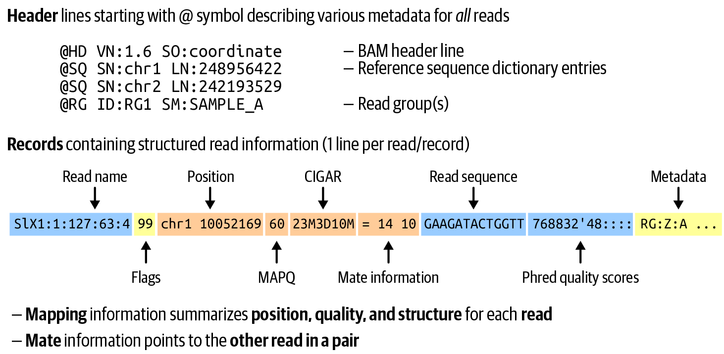
Figure 2-14. Key elements of the SAM format: file header and read record structure.
Note
Unlike SAM and BAM, CRAM is not a real acronym; it was so named to follow the SAM/BAM naming pattern and as a play on the verb to cram, but the CR does not spell out to anything meaningful.
In the SAM/BAM/CRAM format, the read’s local alignment is encoded in the Concise Idiosyncratic Gapped Alignment Report (CIGAR) string. Yes, someone really wanted it to spell out CIGAR. Briefly, this system uses single-letter operators to represent the alignment relationship of one or more bases to the reference with a numerical prefix that specifies how many positions the operator describes in such a way that the detailed alignment can be reconstructed based solely on the starting position information, the sequence, and the CIGAR string.
For example, Figure 2-15 shows a read that starts with one soft-clipped (ignored) base (1S), then four matching positions (4M), one deletion gap (1D), another two matches (2M), one insertion gap (1I), and, finally, one last match (1M). Note that this is a purely structural description that is not intended to describe sequence content: in the first stretch of matches (4M), the third base does not match the reference, so all it means is that “there is a base in position 4.”
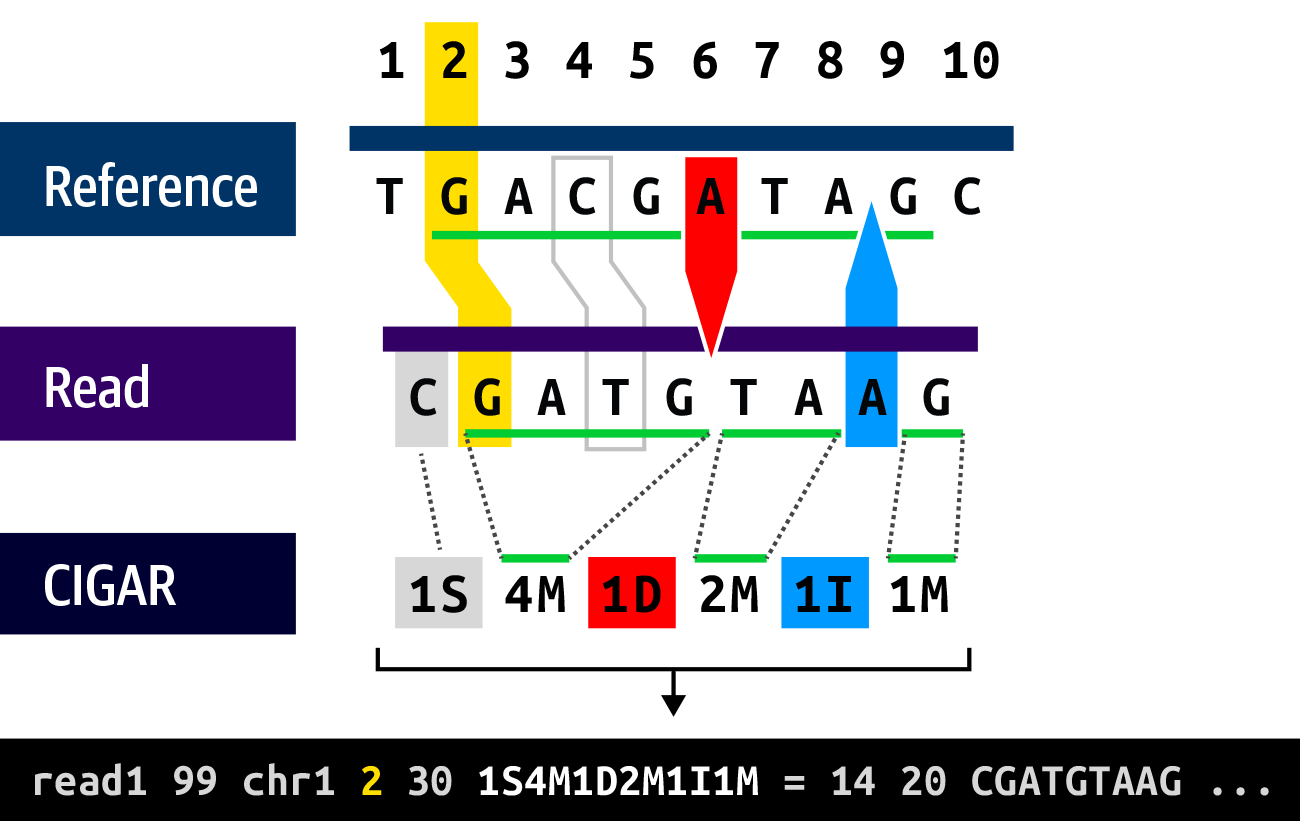
Figure 2-15. The CIGAR string describes the structure of the read alignment.
Let’s come back briefly to that soft clip shown in Figure 2-15, which we qualified as “ignored.” Soft clips happen at the beginning and/or at the end of a read when the mapper isn’t able to align one or more bases to its satisfaction. The mapper basically gives up and uses the soft clip symbol to indicate that those bases do not align to the reference and should be ignored in downstream analysis. As you’ll see in Chapter 5, some of the data that ends up in soft clips is recoverable and can be useful.
Note
Technically, it is possible to store read data in BAM format without including mapping information, as we describe in Chapter 6.
Note that the long-term storage of large amounts of sequence data is a problem that preoccupies large sequencing centers and many funding agencies, and has prompted various groups to propose alternative formats to FASTQ and SAM/BAM/CRAM. However, none has so far managed to gain traction with the wider community.
The amount of read data produced for a single experiment varies according to the type of library as well as the target coverage of the experiment. Coverage is a metric that summarizes the number of reads overlapping a given position of the reference genome. Roughly, this rolls up to the number of copies of the original DNA represented in the DNA library. If this confuses you, remember that the library preparation process involves shredding DNA isolated from many cells in a biological sample, and the shredding is done randomly (for most library preparation techniques), so for any given position in the genome, we expect to obtain read pairs from multiple overlapping fragments.
Speaking of libraries, let’s take a closer look at our options on that front.
Types of DNA Libraries: Choosing the Right Experimental Design
There are about as many ways to prepare DNA libraries as there are molecular biology reagents companies. Generally, though, we can distinguish three main approaches that determine the genomic territory made available to sequencing and the major technical properties of the resulting data: amplicon generation, whole genome preparation, and target enrichment, which is used to produce gene panels and exomes, as depicted in Figure 2-16.
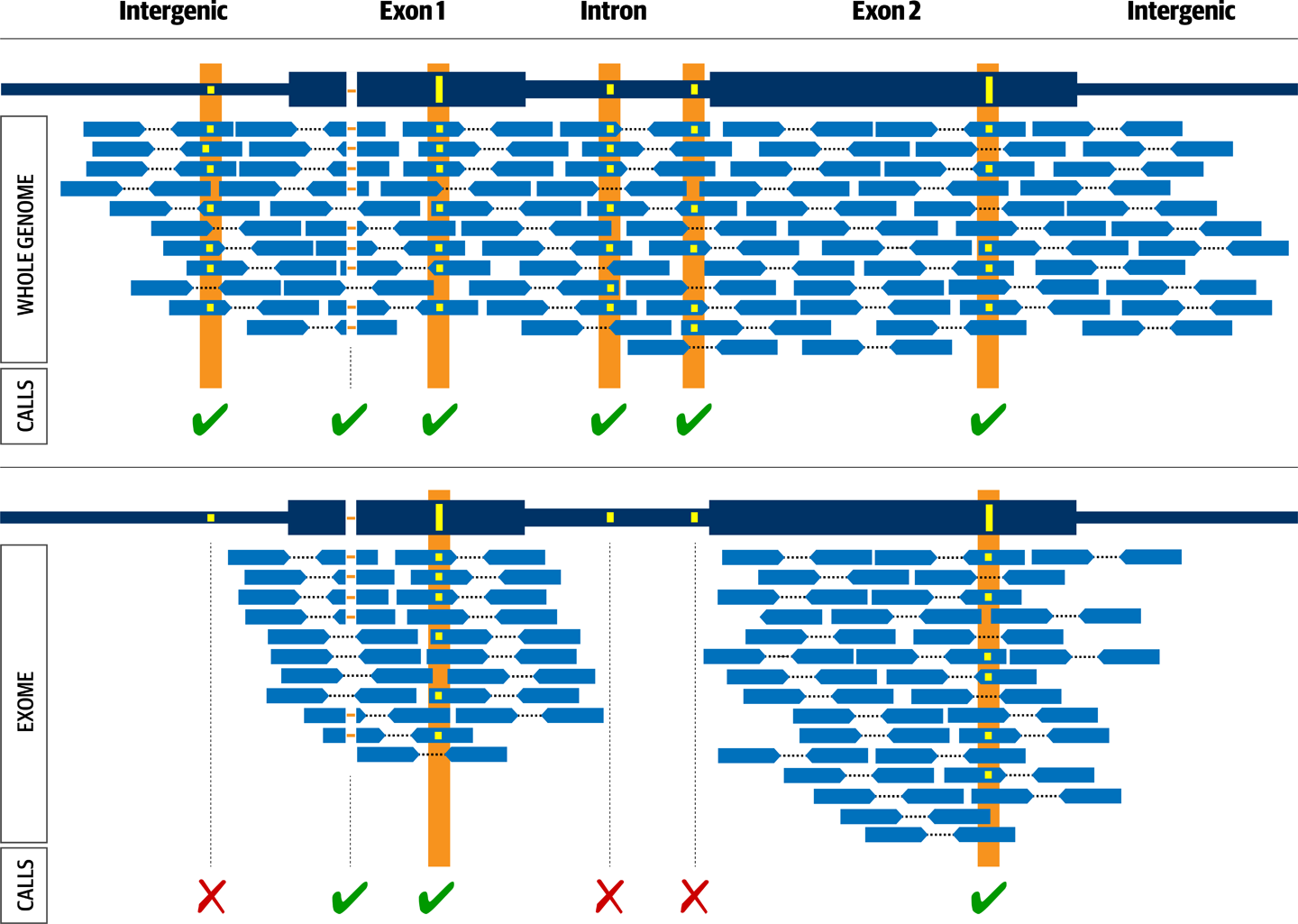
Figure 2-16. Experimental design comparison between whole genome (top) and exome (bottom).
The whole genome library shown in Figure 2-16 will lead to sequence coverage across all regions (exon, intron and intergenic), while the exome library will only lead to coverage across the targeted regions, typically corresponding to exons.
Amplicon preparation
This family of DNA preparation techniques relies on classic polymerase chain reaction (PCR) amplification (either using specifically designed primers or using restriction enzyme sites) to produce amplicons, fragments of DNA present in large numbers of copies that start and stop at the same positions. This means that the territory made available for sequencing is typically very small and dependent on the starting and stopping points we predetermine with our primers or restriction enzymes.
This approach is fairly economical for small-scale experiments and does not require a reference genome, making it a popular option for the study of nonmodel organisms. However, it produces data with enormous PCR-related technical biases. As a result, this approach lends itself very poorly to variant discovery analysis when done with the GATK and related tools; thus, we don’t cover it further in this book.
Whole genome preparation
As the name implies, the goal of whole genome preparation is to sequence the entire genome. It involves putting the DNA through a mechanical shearing process that rips it into a multitude of small fragments and then “filtering” the fragments based on their size to keep only those within a certain range, typically 200 to 800 base pairs. Because a DNA sample contains many copies of the genome and the shearing process is random, we expect that the resulting fragments will be tiled redundantly across the entire genome. If we sequence each fragment once, we should see every base in the genome multiple times.
In practice, some parts of the genome are still very difficult to make available to the sequencing process. Within our cells, our DNA isn’t simply floating around, loosely unfurled; much of it is tightly rolled up and packaged with protein complexes. We can relax it to a point with biochemical persuasion, but some areas remain quite difficult to “liberate.” In addition, some parts of the chromosomes such as the centromere (the middle bit) and telomeres (the bits at the ends) contain vast stretches of highly repetitive DNA that is difficult to sequence and assemble faithfully. The human genome reference is actually incomplete in those areas, and specialized techniques are necessary to probe them. All this to say, when we talk about whole genome sequencing, we mean all of the parts that we can readily access. Nevertheless, even with those limitations, the amount of territory covered by whole genome sequencing is enormous.
Target enrichment: gene panels and exomes
Target enrichment approaches are an attempt at a best-of-both-worlds solution: they allow us to focus on the subset of the genome that we care about, but in a way that is more efficient than amplicon techniques and, to some extent, less prone to technical issues. Briefly, the first step is the same as for whole genome preparation: the genome is sheared into fragments, but then the fragments are filtered not based on size but on whether they match a location we care about. This involves using bait sequences, which are designed very much like PCR primers but immobilized on a surface to capture targets of interest, typically a subset of genes (for gene panels) or all annotated exons (for exomes). The result is that we produce patches of data that can inform us about only those regions that we managed to capture.
One often overlooked downside of this very popular approach is that the manufacturers of commercial kits for generating panel and exome data use different sets of baits, sometimes with important differences in the targeted regions, as illustrated in Figure 2-17. This causes batch effects and makes it more difficult to compare the results of separate experiments that used different target regions.

Figure 2-17. Different exome preparation kits can lead to important differences in coverage location and quantity.
Note
Exome sequencing is sometimes referred to as Whole Exome Sequencing (WES) out of a misguided attempt to contrast it with Whole Genome Sequencing (WGS). It’s misguided, because the contrast is already in the name: the point of the exome is that it’s a subset of the whole genome. Calling it the whole exome is simply unnecessary and arguably inaccurate, to boot.
Whole genome versus exome
So which one is better? The most balanced thing we can say is that these approaches yield qualitatively and quantitatively different information, and each comes with specific limitations. Exome sequencing has proved extremely popular because for a long time it was much cheaper and faster than genomes, and for many common applications such as clinical diagnostics, it was usually sufficient to provide the necessary information. However, this approach suffers from substantial technical issues, including reference bias and unevenness of coverage distribution, which introduce many confounding factors into downstream analyses.
From a purely technical perspective, the data produced by WGS is superior to targeted datasets. It also empowers us to discover biologically important sequence conformations that lurk in the vast expanses of genomic territory that do not encode genes. Thanks to falling costs, whole genome sequencing is now becoming popular, though the downside is that the much larger amount of data produced is more challenging to manage. For example, a standard human exome sequenced at 50X coverage takes about 5 GB to store in BAM format, whereas the same person’s whole genome sequenced at 30X coverage takes about 120 GB.
If you have not worked with exomes or whole genomes before, the difference between them can seem a bit abstract when we’re talking about amounts of data, file sizes, and coverage distributions. It can be really helpful to look at a few files in a genome browser to see what this means in practice. As shown in Figure 2-18, the whole genome sequencing data is distributed almost uniformly across the genome, whereas the exome sequencing data is concentrated in localized piles. If you look at the coverage track in the genome viewer, you’ll see the coverage profile for the whole genome looks like a distant mountain range, whereas the profile for the exome looks like a volcanic island in the middle of a flat ocean. This is an easy and surprisingly effective way to distinguish the two data types by the naked eye. We show you how to view sequencing data in the Integrated Genome Viewer (IGV) in Chapter 4.
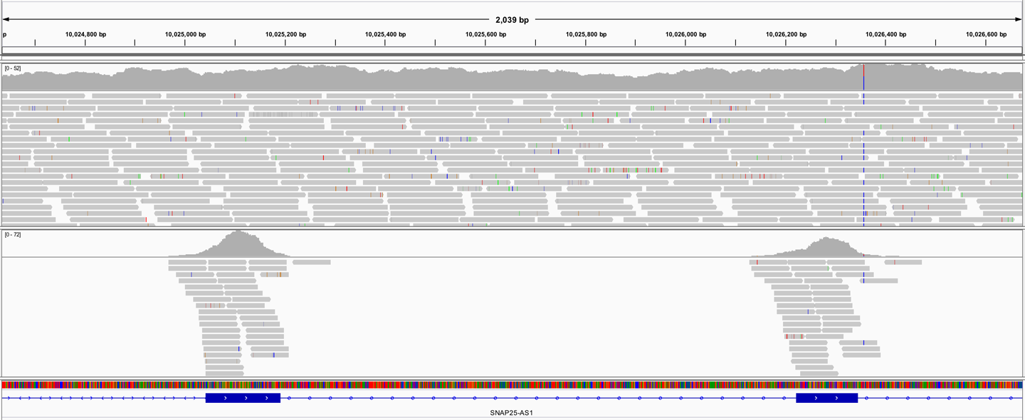
Figure 2-18. Visual appearance of whole genome sequence (WGS, top) and exome sequence (bottom) in a genome browser.
Most of the exercises in this book use whole genome sequencing data, but we also provide pointers to resources for analyzing exome data, and in Chapter 14 we go through a case study involving exomes.
Data Processing and Analysis
Finally, we get to the computational part! Now, you might think that as soon as we have the sequence data in digital form, the real fun begins. However, there is a twist: the data produced by the sequencers is not directly usable for variant discovery analysis: it’s a huge pile of short reads, and we don’t know where they came from in the original genome. In addition, there are sources of bias and errors that are likely to cause problems in downstream analysis if left untreated. So we’re going to need to apply a few preprocessing steps before we can get to the genomic analysis proper. First, we map the read data to a reference genome and then we apply a couple of data cleanup operations to correct for technical biases and make the data suitable for analysis. Next, we’ll finally be able to apply our variant discovery analysis workflows. In this section, we go over the core concepts involved in genome mapping (aka alignment) and variant calling, but we leave the rest for Chapter 6. We also touch briefly on data quality issues that can interfere in variant discovery analysis.
Mapping Reads to the Reference Genome
Ideally, we’d like to reconstruct the entire genome of the individual we’re working on to compare it to the reference, but we don’t have the sample in one piece—it’s more like a million pieces, as illustrated in Figure 2-19!
Well, actually 360 million for a standard 30X WGS, and 30 million for a standard 50X Exome, according to the Lander-Waterman equation. It’s quite the jigsaw puzzle. And, by the way, the pieces overlap 30 to 50 times (depending on target depth).
So the goal of the mapping step is to match each read to a specific stretch of the reference genome. The output is a BAM file that has mapping and alignment information encoded in each read record, as described in “High-Throughput Sequencing Data Generation”.
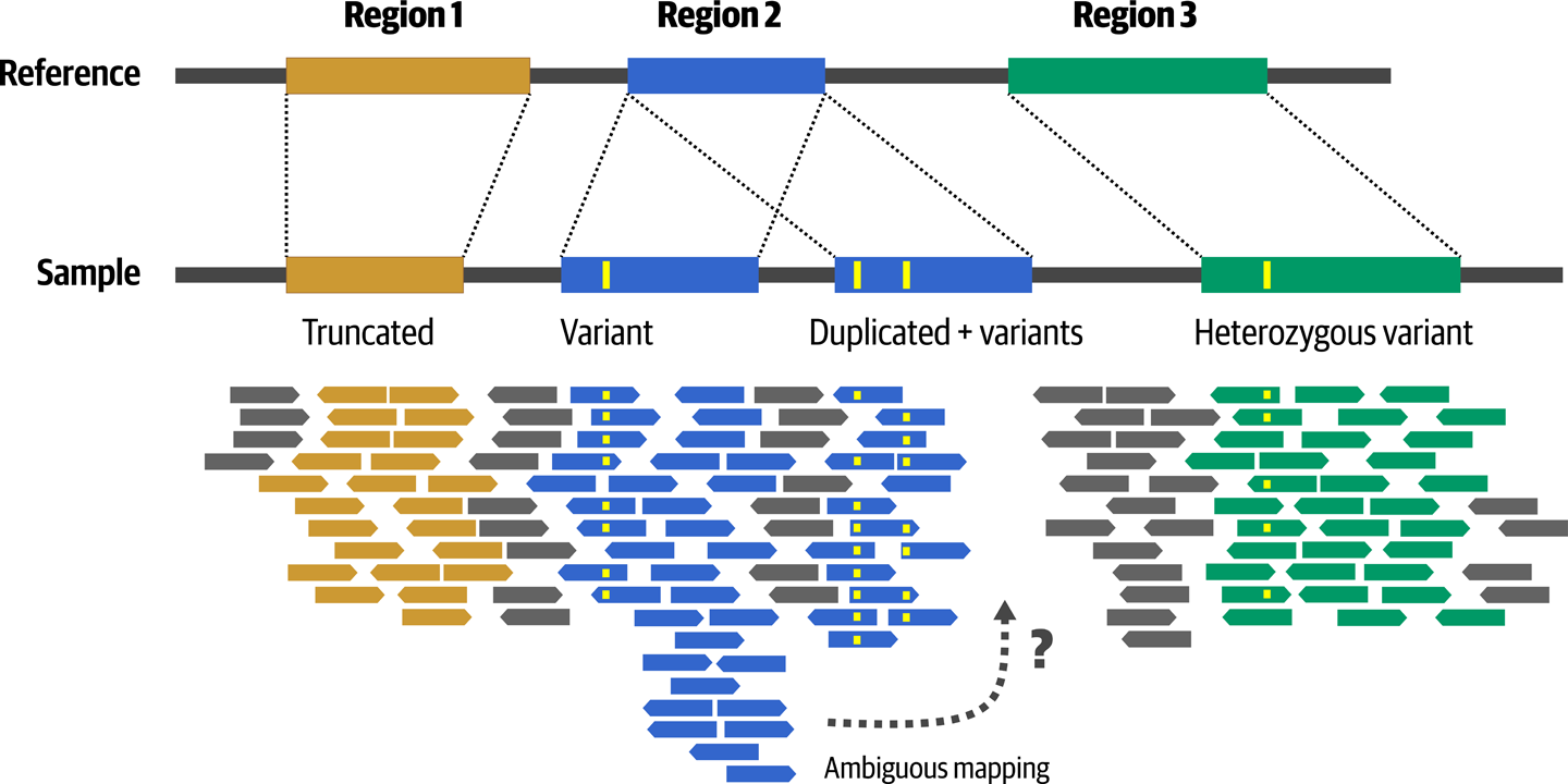
Figure 2-19. Sequence divergence introduces mapping challenges and ambiguity.
This is often called alignment because it outputs detailed alignment information for each read, but it is arguably more appropriate to call it mapping. Genome mapping algorithms are primarily designed to solve that fundamental problem of identifying the best matching location for a very small string of letters (typically ~150 to ~250) against an enormously huge one (about three billion for humans, not counting alternate contigs). Among other neat tricks, this involves using a scoring system that penalizes gaps. However, this has drawbacks when it comes to producing the fine-grained letter-by-letter alignment. The mapper works on one read at a time, so it is not well equipped to deal with naturally occurring sequence features like large insertions and deletions, and it will often prefer to clip sequences off the end of a read rather than introduce a large indel. We look at an example of this in Chapter 5 when we introduce GATK and its flagship germline short variant caller, HaplotypeCaller. What is important to understand at this point is that we trust the mapper to place the reads in the appropriate places most of the time, but we can’t always trust the exact sequence alignments it produces.
As noted in Figure 2-19, an additional complication is that some genomic regions are copies of ancestral regions that were duplicated. The sequence of copies may be more or less divergent depending on how long ago the duplication happened and how many other mutation events produced variants in the copies. This makes the mapper’s job more difficult because the existence of competing copies introduces ambiguity as to where a particular read might belong. Thankfully, most short read sequencing is now done using paired-end sequencing, which helps resolve ambiguity by providing additional information to the mapper. Based on the protocol used for library preparation, we know that we can expect DNA fragments to be within a certain size range, so the mapper can evaluate the likelihood of possible mapping locations based on the distance between the two reads in the pair, as shown in Figure 2-20. This does not apply for long-read sequencing technologies such as PacBio and Oxford Nanopore, for which the longer length of the reads typically leaves less opportunity for ambiguity by reading all the way through repeat regions.
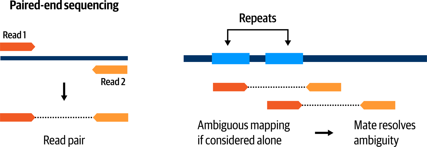
Figure 2-20. Paired-end sequencing helps resolve mapping ambiguity.
Note
Fragments of DNA generated during library preparation are sometimes called inserts because older preparation techniques involved inserting each fragment into a small circular piece of DNA called a plasmid. As a result, the relevant quality-control metric is usually called insert size even though nowadays the library preparation no longer involves insertion into plasmid vectors.
As noted a moment ago, a few other processing steps are needed to clean up the aligned data before we would normally move on to variant calling. We cover them later; for now, it’s time to finally tackle the beast that is going to follow us through just about every chapter in this book.
Variant Calling
The term variant calling is thrown around a lot and is sometimes used to refer to the entire variant discovery process. Here we’re defining it narrowly as the specific step in which we identify potential variants by looking for evidence of a particular type of variation in the available sequence data. The output of this step is a raw callset, or set of calls, in which each call is an individual record for a potential variant, describing its position and various properties. The standard format for this is the VCF, which we describe in the next sidebar.
The nature of the evidence we use to identify variants is different depending on the type of variant we’re looking for.
For short sequence variants (SNVs and indels), we’re comparing the specific bases in short stretches of sequence. In principle, it’s quite straightforward: we produce a pileup of reads, compare them to the reference sequence, and identify where there are mismatches. Then we simply count the numbers of reads supporting each allele to determine genotype: if it’s half and half, the sample is heterozygous; if it’s all one or the other, the sample is homozygous reference or homozygous variant. For example, the IGV screenshot in Figure 2-22 shows a probable 10-base deletion (left), a homozygous variant SNP (middle right), and a heterozygous variant SNP (rightmost) in whole genome sequence data.
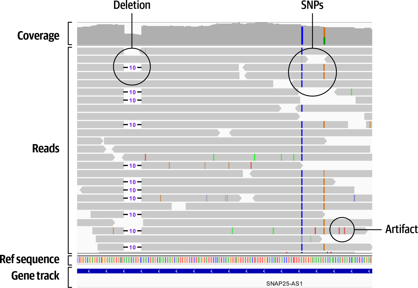
Figure 2-22. Pileup of reads in IGV showing several probable short variants.
For copy-number variants, we’re looking at the relative number of sequence reads produced across multiple regions. Again, it’s a fairly simple reasoning on the surface: if a region of the genome is duplicated in a sample, when we go to sequence that sample, we’re going to generate twice as many reads that align to that region, as demonstrated in Figure 2-23.
And for structural variants, we’re looking at a combination of both base-pair resolution sequence comparisons as well as relative amounts of sequence.
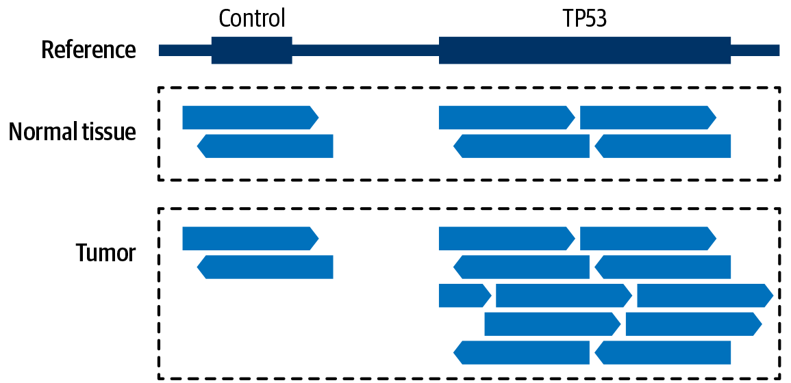
Figure 2-23. Relative amounts of coverage provide evidence for copy-number modeling.
In practice, the process for identifying each of the variant types confidently is rather more complicated than the simple logic that we just outlined, largely because of various sources of error and uncertainty that muddy the waters, which we touch on shortly. That’s why we’ll want to apply more robust statistical approaches that take various sources of error into account; some through empirically derived heuristics, and others through modeling processes that do not require prior knowledge of what kinds of errors might be present in the data.
We can rarely say definitively, “this call is correct” or “this call is an error,” so we express results in probabilistic terms. For each variant call output by the program, the caller will assign scores that represent how confident we can be in the result. In the earlier indel example, the variant quality (QUAL) score of 50 means “there is a 0.001% chance that this variant is not real” and the genotype quality (GT) score of 17 for the second sample means “there is a 1.99% chance that this genotype assignment is incorrect.” (We cover the distinction between variant quality and genotype quality in more detail in Chapter 5.)
Variant calling tools typically use some internal cutoffs to determine when to emit a variant call or not emit one depending on these scores. This avoids cluttering the output with calls that are grossly unlikely to be real. However, it’s important to understand that those cutoffs are usually designed to be very permissive in order to achieve a high degree of sensitivity. This is good because it minimizes the chance of missing real variants, but it does mean that we should expect the raw output to still contain a number of false positives—and that number can be quite large. For that reason, we need to filter the raw callset before proceeding to further downstream analysis.
Filtering variants is ultimately a classification problem: we’re trying to distinguish variants that are more likely to be real from those that are more likely to be artifacts. The more clearly we can make this distinction, the better chance we have of eliminating most of the artifacts without losing too many real variants. Therefore, we’ll evaluate every filtering method based on how favorable a trade-off it enables us to make, expressed in terms of sensitivity, or recall (percentage of the real variants that we’re able to identify), and specificity, or precision (the percentage of the variants we called that are actually real), as depicted in Figure 2-24.
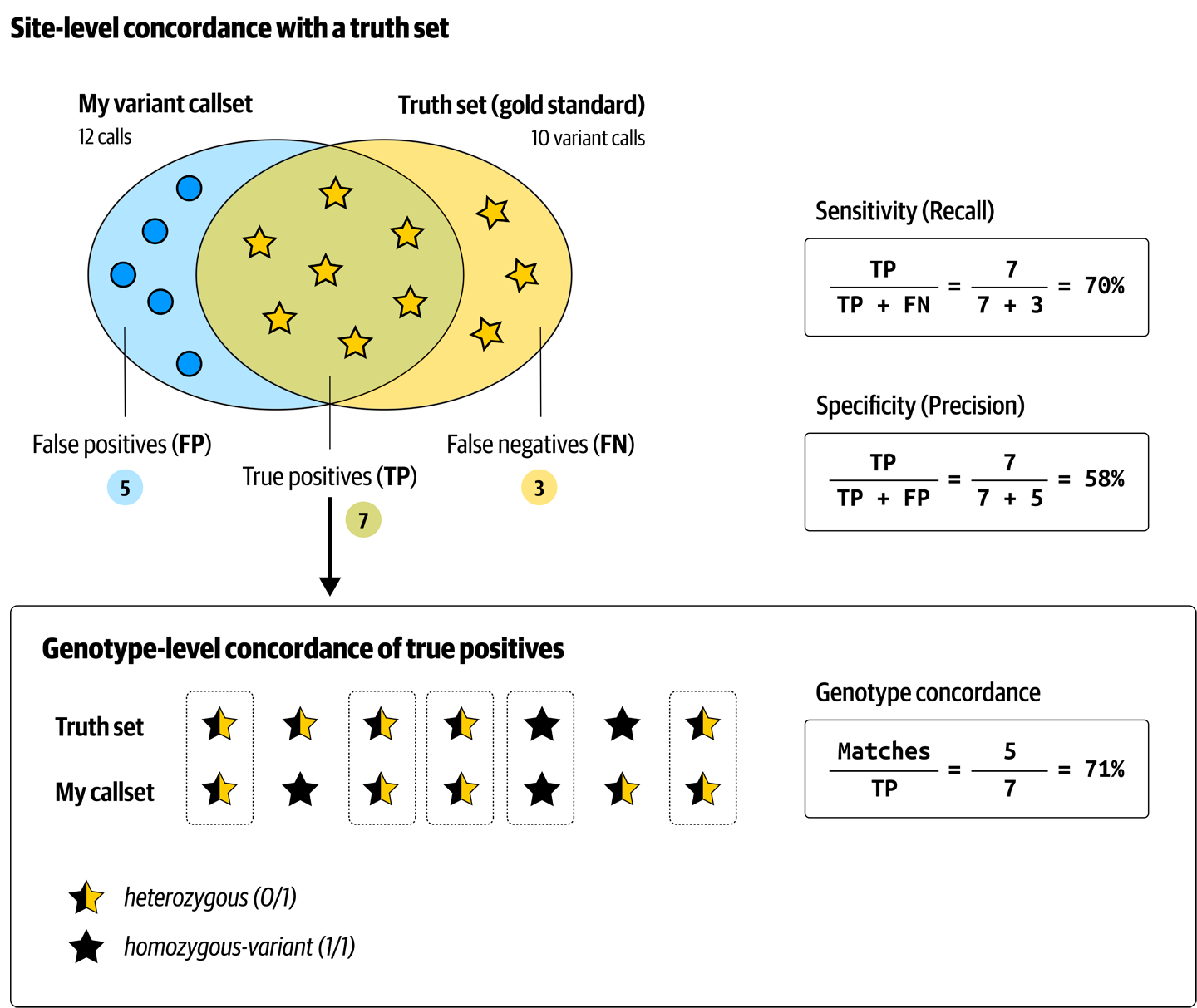
Figure 2-24. Cheat sheet of variant metrics.
There are many approaches to filtering variants, and the choice of what is appropriate depends not only on the variant class we’re looking at, but also on the type and quality of the prior knowledge we have about genomic variation in the organism we study. For example, in humans we have extensive catalogs of variants that have been previously identified and validated, which we can use as a basis for filtering variant calls in new samples, so we can use modeling approaches that rely on the availability of training data from that same organism. In contrast, if we’re looking at a nonmodel organism that is being studied for the very first time, we do not have that luxury and will need to fall back on other methods.
Data Quality and Sources of Error
A lot of things can go wrong (Figure 2-25) during the entire process, from initial sample collection all the way to the application of computational algorithms, with multiple sources of error and confounding factors creeping in at each stage. Let’s review the most common, which are important for understanding many of the procedures that we’ll apply in the course of genomic analysis.
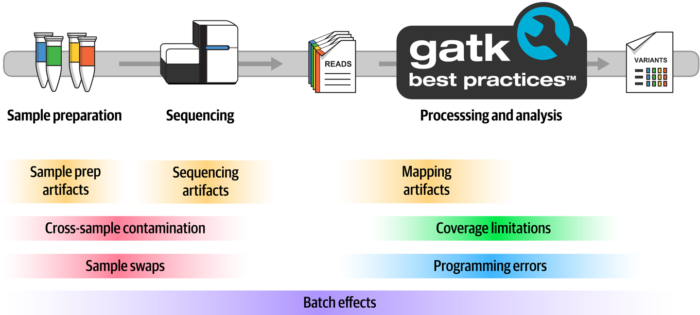
Figure 2-25. Common sources of error in variant discovery.
Contamination and sample swaps
At the earliest stages of sample collection and preparation, we are vulnerable to several types of contamination. The most difficult to prevent is contamination by foreign material, especially in the case of cheek swabs and saliva samples. Think about what’s going on in your own mouth right now. When is the last time you brushed your teeth? What did you have for lunch? Any chance you have a bit of a cold at the moment, maybe a runny nose? If we were to try to sequence your genome based on a saliva sample or cheek swab, whatever is in your mouth is going to be sequenced along with your own DNA. At the very least, this means some of the resulting sequence data will be useless noise; in worst-case scenarios, it can cause errors in the downstream analysis results.
Then there’s cross-sample contamination, which people don’t like to talk about because it implies something went wrong either with the quality of equipment or the skill of the person doing the work. But the reality is that cross-contamination between samples happens often enough that it should be addressed in the analysis. It can happen during the initial sample collection, especially when sampling is done in the field in less than ideal conditions, or during library preparation steps. The result in either case is that some genetic material from person A ends up in the tube for sample B. When the level of contamination is low, it’s typically not a problem for germline variant analysis, but as you’ll see in Chapter 7, it can have major implications for somatic analysis. Also in Chapter 7, we discuss how we can detect and handle cross-sample contamination in the somatic short variant pipeline.
Finally, sample swaps generally come down to mislabeling—either the label ending up on the wrong tube, or handwritten labels with ambiguous lettering—or metadata handling errors during processing. To detect any sample swaps that occur during processing, the best practice recommendation is to put inbound samples through a fingerprinting procedure and then check processed data against the original fingerprints to detect any swaps.
Biochemical, physical, and software artifacts
Various physical and biochemical effects that occur during sample preparation (such as shearing and oxidation) can cause DNA damage that ultimately translates into having the wrong sequence in the output data. Library preparation protocols that involve a PCR amplification step introduces similar errors because our good friend, the polymerase, is wonderfully productive but prone to incorporating the wrong base. And, of course, sometimes the sequencing machine fails to read the light signals bouncing off the DNA accurately, producing either low-confidence BCLs or outright errors. So the data we have might not always be of the highest quality.
Some biochemical properties of sequence context affect the efficiency of library preparation, flowcell loading, and sequencing processes. This results in producing artificially inflated coverage in some areas and inadequate coverage in others. For example, and as Figure 2-26 shows, we know that stretches of DNA with high GC content (areas with lots of G and C bases) will generally show less coverage compared to the rest of the genome. Highly repetitive regions are also associated with coverage abnormalities.
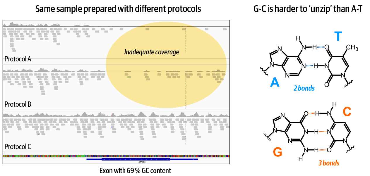
Figure 2-26. Some biochemical properties of the DNA itself cause biases in certain regions.
Then, after the data has been generated and we go to process it, we run into other sources of error. For example, mapping artifacts caused by the biological complexity of the genome (spoiler: it’s a mess) can lead to reads ending up in the wrong place, supporting apparent variants that are not real. Shortcuts in algorithms made to improve performance can cause small approximations to balloon into errors. And although we’re sad to say this, software bugs are inevitable.
The cherry on the cake, finally, consists of batch effects—because we can deal with a certain amount of error as long as it’s consistent across all the samples we’re comparing, but the minute we begin comparing results from samples that were processed differently, we’re in the danger zone. If we’re not careful, we could end up ascribing biological impact to an artifact that just happens to be present in a subset of our samples because of how they were processed.
Functional Equivalence Pipeline Specification
The data preprocessing phase that takes place before variant calling is probably the part of genomic analysis that has the most heterogeneity in terms of valid alternative implementations. There are many ways you can “do it right” depending on how you want to handle the logistics side, whether you care more about cost or runtime, and so on. For each step, several alternative software tools (some open source, some proprietary) are available for you to use—especially for mapping. It’s almost a rite of passage for newly minted bioinformatics developers to write a new mapping algorithm.
However, there is a dark side to this abundance of choice. Differences between implementations can cause subtle batch effects in downstream analyses that compare datasets produced by those variant pipelines, sometimes with important consequences for the scientific results. That is why historically the Broad Institute teams have always chosen to redo the preprocessing on genomic data coming in from external sources. They would systematically revert any aligned read data back to an unmapped state and scrub it clean of any tagging or any reversible modifications. Then, they would put the reverted data through their internal preprocessing pipeline.
That strategy is unfortunately no longer sustainable given the huge increase in the amount of data being produced and used in large aggregation projects such as gnomAD. To address this issue, the Broad Institute teamed up with several of the other largest genome sequencing and analysis centers in North America (New York Genome Center, Washington University, University of Michigan, Baylor College of Medicine) to define a standard for standardizing pipeline implementations. The idea is that any data processed through a pipeline that conforms with the specification will be compatible, so that any datasets aggregated from multiple conformant sources can be analyzed together without fear of batch effects.
The consortium published the Functional Equivalence specification and encourages all genome centers as well as anyone else who is producing data, even at a small scale, to adopt the specification in order to promote interoperability and eliminate batch effects from joint studies.
Wrap-Up and Next Steps
This concludes our genomics primer; you now know everything you need on the scientific side to get started with GATK and variant discovery. Next up, we do the equivalent exercise on the computational side with a technology primer that takes you through the key concepts and terminology you need to know to run the tools involved.