Chapter 7. GATK Best Practices for Somatic Variant Discovery
In this chapter, we tackle somatic variant discovery, mainly as it applies to cancer research. This is going to introduce new challenges and, correspondingly, new experimental and computational designs. We begin with somatic short variants, which still have a lot in common with germline short variants, with enough new challenges to keep things interesting. Then we expand our horizons to include copy-number variation, which involves a very different approach from what we’ve taken so far.
Challenges in Cancer Genomics
Before we get into the weeds, let’s make one thing clear: everything is more difficult with respect to cancer. Consider what is happening in the body before a tumor even begins to develop. Living cells in our bodies are not static; they are metabolically active, taking in nutrients, doing work, and pumping out waste. Some of them are dividing at various rates. Enzymes are unraveling DNA to transcribe it and/or copy and repackage it. At the scale of a single cell, very few of those molecular transactions ever go wrong, but because this is happening all the time in millions of cells, the numbers add up to a lot of little things going wrong, causing mutations across the board.
Most of the time, these mutations have no discernible effect whatsoever. But from time to time, a mutation arises that destabilizes the affected cell’s metabolism in a way that causes it to begin dividing more rapidly and produce a tumor. That’s still not cancer yet, mind you; most tumors in our bodies remain relatively contained and harmless. However, some then experience other destabilizing mutations that kick off a chain reaction, leading to cancerous development, including aggressive growth and in the worst-case scenario, metastasis: dissemination to other parts of the body. The mutation events that drive this progression are appropriately called driver mutations, in contrast to the others, which are called passenger mutations. Driver mutations are typically the main focus of somatic analysis in cancer research.
The difficulty here is that as the tumor progresses, various metabolic functions begin to break down and the cells lose their ability to repair damaged DNA. As a result, the frequency of mutation events increases, and variants accumulate in a variety of divergent cell lineages, producing a highly heterogeneous environment. When a pathologist samples the tumor tissue, they end up extracting a mix of multiple cell lines instead of the well-behaved population of largely clonal cells that you expect from healthy tissue.
This is a huge problem for detecting somatic variation, because depending on the internal state of the tumor tissue at the time we sample it, the variants caused by driver mutations might be represented at only a low fraction of the total genomic material. The most direct consequence is that we can’t allow the variant caller to make any assumptions about the fraction of variant allele that we expect to find. This is a big difference compared to the germline case, in which variant allele fractions should roughly follow the ploidy of the organism. That is why we use different variant callers for somatic versus germline variant discovery analysis, which, under the hood, use different algorithms to model genomic variation in the data.
In addition, the sampling process itself introduces confounding factors. Depending on the skill of the pathologist, the stage of progression of the tumor, and the type of biological tissue affected, we can end up with a tumor sample that is contaminated with healthy “normal” cells. Conversely, if we are able to obtain a matched normal sample, a sample taken from supposed healthy tissue from the same person—that sample can, in fact, be contaminated with low levels of tumor cells, as depicted in Figure 7-1.
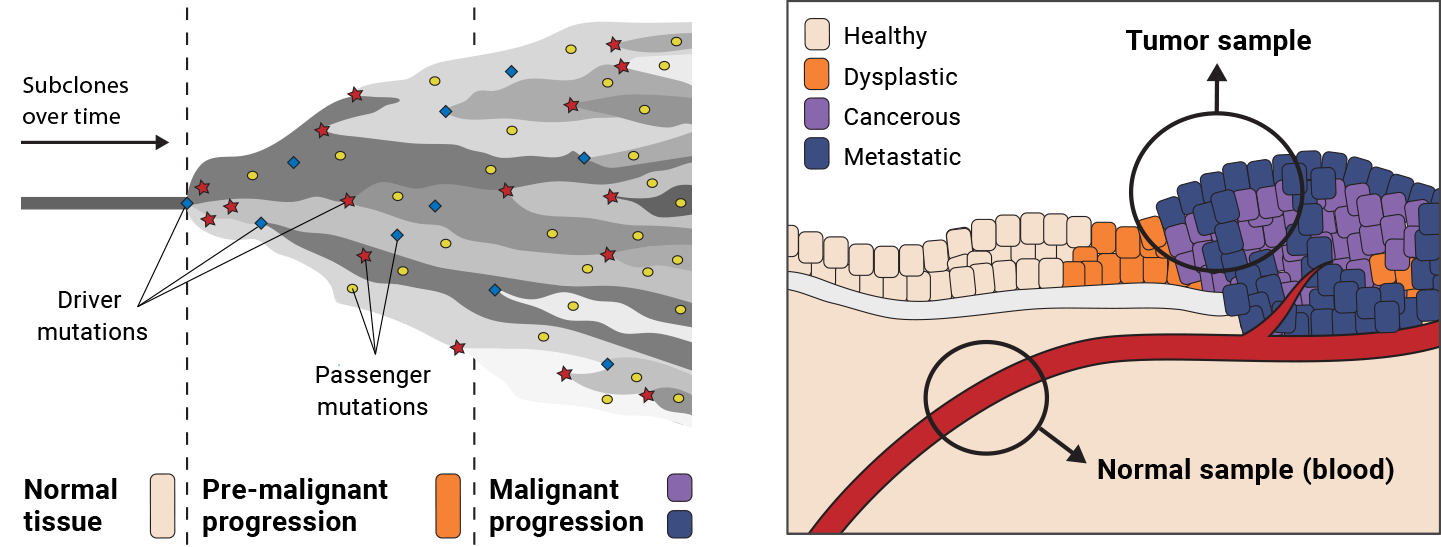
Figure 7-1. Tumor progression leads to heterogeneity (left); sampling is difficult (right).
The practical consequence of all this for somatic variant analysis is that our work will necessarily be deeply vulnerable to sources of contamination and error because the signal we are trying to detect is much lower compared to the noise that is present in the data, particularly in the case of advanced cancers.
Somatic Short Variants (SNVs and Indels)
Let’s commence our exploration of somatic variant calling with short variants—SNVs and indels. Some of the core concepts we cover here should feel familiar if you’ve already worked through Chapter 6, and indeed some of the tools and underlying algorithms are the same. As we’ve done previously, we’ll be looking at piles of reads and their exact sequences to identify substitutions and small insertions and deletions.
However, the basic experimental design that we follow is actually very different. In germline variant discovery, we were mainly interested in identifying variants that were present in some people but not in others, which led us to favor the joint calling approach. In somatic variant discovery, we’re primarily looking for differences between samples coming from the same person, so we will shift our focus to a different paradigm: the Tumor-Normal pair analysis.
The most useful source of information for identifying somatic short variants in the context of cancer is the comparison of the tumor against a sampling of healthy tissue from the same individual, which, as we said previously, is called a matched normal, or often normal for short. The idea here is that any variation observed in the normal sample is part of the germline genome of the individual and can be discounted as background, whereas any variant observed in the tumor sample that is not present in the normal sample is more likely to be a somatic mutation, as demonstrated in Figure 7-2.
Unfortunately, some confounding factors muddy the waters. For example, biopsy samples preserved with formalin and paraffin, a widely used laboratory technique (FFPE, for formalin-fixed paraffin-embedded), are subject to biochemical alterations that happen during sample preparation and cause patterns of false-positive variant calls that are specific to the tumor sample. Conversely, the presence of tumor cells in normal tissue (either due to contamination during sampling or metastatic dispersion) can cause real somatic variants to be erroneously discounted as being part of the germline of the individual. Finally, as we discussed earlier, the various sources of technical error and contamination that affect all high-throughput sequencing techniques to some degree will have a proportionately higher impact on somatic calling. So, we will need to apply some robust processing and filtering techniques to mitigate all these problems. (The overall workflow is illustrated in Figure 7-3.)
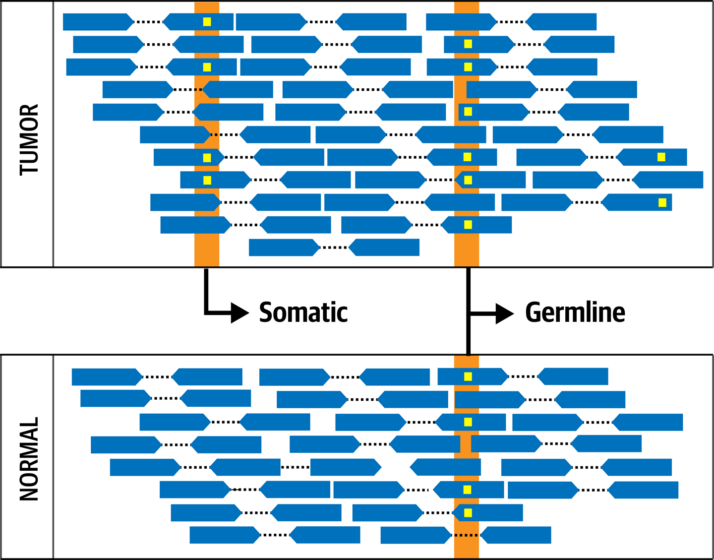
Figure 7-2. The fundamental concept of Tumor-Normal comparison.
Before we get into the details of the Tumor-Normal workflow in the next subsection, it’s important to note that sometimes it’s not possible to apply the full Tumor-Normal pair analysis to a sample or set of samples, usually because we simply don’t have matched normals for them. This is particularly frustrating when that lack comes from an investigator’s failure to collect a matched normal from the participant or patient. Such cases highlight the importance of making sure that researchers map out the full analysis protocol before engaging in data collection. On the other hand, in some cases it’s biologically impossible to obtain a matched normal; for example, blood-borne cancers typically reach every tissue in the body, so we can’t assume that any tissue sample would constitute an appropriate normal.
Whatever the reason for the absence of a matched normal, the workflow that we present in the next subsection can be run on a tumor sample with only a few minor modifications, which are detailed in the online GATK documentation. However, you should be aware that the results will necessarily be noisier because you will be relying on the germline population resource to exclude the person’s own germline genome.
Overview of the Tumor-Normal Pair Analysis Workflow
This workflow, illustrated in Figure 7-3, is designed to be applied to a tumor sample and its matched normal. We can apply it equally to whole genome data as well as exome data, but both the tumor and the normal must be of the same data type and have been run through the same preprocessing workflow, as we described for germline variant discovery.
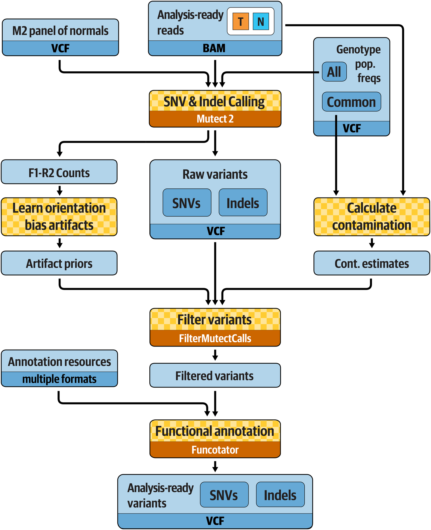
Figure 7-3. Best Practices for somatic short variant discovery.
The main variant calling step, which involves a tool called Mutect2, is applied on both the tumor and the normal sample, with the addition of two important resources: a Panel of Normals (PoN) and a database of germline population frequencies of all germline variants that have been previously reported. The PoN is a resource that allows us to eliminate common technical artifacts; we dedicate the next subsection to explaining how it works and how to create one, although you won’t run it yourself for practical reasons. We talk about the germline population frequencies resource in “Filtering Mutect2 Calls”. The filtering process will take into account read orientation statistics, an estimate of cross-sample contamination, germline background, and concordance with the PoN. Finally, we apply functional annotation to the variant callset to predict the effect of candidate variants.
Creating a Mutect2 PoN
The PoN is a callset in VCF format that aims to capture common recurring artifacts, so we can filter those out if we encounter them in our tumor data. We generate it by running the somatic caller, Mutect2, on a set of normal samples that were produced with the same sequencing and library preparation technologies as our tumor sample. The idea is that we’re asking the caller to show us everything it could consider a somatic variant, excluding obvious germline variants (unless otherwise specified). Because these are normals, not tumor samples, we can reasonably assume that any variant calls that are produced this way are either germline variants or artifacts. For those that are more likely to be artifacts, we can therefore further assume that if we see the same artifacts in multiple normals, they might have been caused by the technological processes involved, so we can expect to see them pop up in some of our tumor samples that were processed the same way. If we do see them, we’ll want to discount their likelihood of being real somatic variants.
Note
The normal samples used for making the PoN usually come from people who are unrelated to the person whose tumor we are analyzing. They can be matched normals from other cancer research participants or germline samples collected from healthy individuals in unrelated research projects, as long as the appropriate consents have been provided. The background genetics of the participants or their population of origin don’t really matter; it’s all about the technical profile of the data. Ideally, we want to include at least 40 samples; most PoNs used for research purposes at the Broad Institute are composed of several hundred samples.
We won’t run the PoN creation commands in this chapter, because they would take too long to run. Instead, we demonstrate usage with some generic command lines. You can find links to full implementations in the GATK Best Practices documentation.
If we were to do this, we would first run Mutect2 in tumor-only mode on the normals selected to be in our PoN. We would do this separately on all the normals in our panel. The following command (and subsequent ones in this section) are just examples; we’ll have you execute commands on your VM a little later:
 gatk Mutect2 \
    -R reference.fasta \
    -I normal_1.bam \
    -O normal_1.vcf.gz \
    --max-mnp-distance 0
This command applies the somatic variant calling model to the normal tissue sample’s BAM file and produces a VCF file of calls that are most likely all either artifacts or germline variants.
Note
The --max-mnp-distance 0 setting disables the tool’s ability to combine neighboring SNVs into multinucleotide variants in order to maximize comparability across all the normals in the PoN that we’re putting together.
Next, we would consolidate all the per-normal VCFs using GenomicsDB, which you might recognize from the germline joint calling workflow. At that time, we were consolidating GVCFs, whereas here we’re working with regular VCFs, but it doesn’t make any difference: the GenomicsDB tools are quite happy to work with either type of VCF:
gatk GenomicsDBImport \
    -R reference.fasta \
    -L intervals.interval_list \
    -V normal_1.vcf.gz \
    -V normal_2.vcf.gz \
    -V normal_3.vcf.gz \
    --genomicsdb-workspace-path pon_db
Finally, we would extract the calls that are relevant to the goals of the PoN. By default, the rule is to keep any variant call observed in two or more samples but below a certain frequency threshold in the germline population resource:
gatk CreateSomaticPanelOfNormals \
    -R reference.fasta \
    -V gendb://pon_db \
    --germline-resource af-only-gnomad.vcf.gz \
    -O pon.vcf.gz
You might recognize gnomAD as the population resource we used in Chapter 6, in the single-sample filtering protocol. The gnomAD database is a public resource that includes variant calls from more than 100,000 people, and for each, it provides the frequency at which each allele is found in the population of the database. We use that information here to gauge the likelihood that a variant call that shows up in several normals in the panel might in fact be a germline variant rather than a recurring artifact.
This generates the final VCF that we will use as a PoN. It does not include any of the sample genotypes; only site-level information is retained. We provide an example PoN that you can examine with good old zcat, grep, and head, as we’ve done previously, if you want to see the structure of the information within the file (execute this command in the /home/book/data/somatic directory inside the GATK container):
# zcat resources/chr17_m2pon.vcf.gz | grep -v '##' | head -3
#CHROM  POS     ID      REF     ALT     QUAL    FILTER  INFO
chr6    29941027        .       G       A       .       .       .
chr6    29941061        .       G       C       .       .       .
Note that this example PoN file includes data only in a subset of regions of interest that are located within chromosome 6, chromosome 11, and chromosome 17.
Running Mutect2 on the Tumor-Normal Pair
Now that you know how to create a PoN, let’s move to the main event of this section, which consists of running Mutect2 on the Tumor-Normal pair using a PoN that we created for you from 40 publicly available normal samples from the 1000 Genomes Project. Just as in Chapter 6, we’re going to do this work within the GATK container on our trusty VM, so turn on your VM if it’s not already running, and spin up the GATK container as we showed you in Chapter 5. This time, however, our working directory is /home/book/data/somatic, and we’ll need to make another sandbox:
# cd /home/book/data/somatic
# mkdir sandbox
We run Mutect2 on the Tumor-Normal pair together, specifying which sample name (as encoded in the SM tag in the BAM file) should be used for the normal with the -normal argument. We provide the PoN and the gnomAD germline resource with the -pon and --germline-resource arguments, respectively. Plus, we specify intervals (using -L and an interval list file) because we’re running on exome data:
# gatk Mutect2 \
    -R ref/Homo_sapiens_assembly38.fasta \
    -I bams/tumor.bam \
    -I bams/normal.bam \
    -normal HCC1143_normal \
    -L resources/chr17plus.interval_list \
    -pon resources/chr17_m2pon.vcf.gz \
    --germline-resource resources/chr17_af-only-gnomad_grch38.vcf.gz \
    -bamout sandbox/m2_tumor_normal.bam \
    -O sandbox/m2_somatic_calls.vcf.gz
This will run for a few minutes, so it’s a good time to take a stretch break. After about five minutes, you should see the completion message from Mutect2:
15:07:19.715 INFO  ProgressMeter - Traversal complete. Processed 285005 total
regions in 5.0 minutes.
This Mutect2 command produces a VCF file containing possible variant calls as well as a bamout file. You might remember the bamout file from the exercises we ran with HaplotypeCaller in Chapter 5; this is the same thing. Mutect2 is built on most of the same code as HaplotypeCaller, and pulls the same graph-based realignment trick to improve sensitivity to indels. The big difference between them is the genotyping model. For more information on their respective algorithms, see the HaplotypeCaller and Mutect2 documentation on GATK’s website. For now, just keep in mind that Mutect2 also realigns the reads, so if we want to look at the read data as part of the variant review process later on, we’ll need the bamout. Because this is something analysts do very frequently for somatic calls (much more, relatively speaking, than for germline calls) we just set the Mutect2 command to produce the bamout systematically.
Estimating Cross-Sample Contamination
As we outlined earlier, identification of somatic mutations is more heavily affected by sources of low-grade noise than the germline case. Even small amounts of contamination between samples (which happens more often than researchers like to think) can confuse the caller and lead to a lot of FPs. Indeed, we have no direct way to distinguish between an allele that shows up in the data because there is a real mutation in the biological tissue, and one that shows up because our sample is contaminated with DNA from someone else who has that allele in their germline.
We can’t directly correct for such contamination, but we can estimate how much it affects any given sample. From there, we can flag any mutation calls that are observed at an allelic fraction equal to or smaller than the contamination rate. It doesn’t mean we rule out those calls as being necessarily false, but it does mean we’ll be extra skeptical of those calls when we move on to the next phase of analysis.
To estimate the contamination rate in our tumor sample, we first identify homozygous-variant sites in the Normal to choose what sites to look at in the Tumor and then evaluate how much contamination we might have in the tumor based on the fraction of reads supporting the reference allele at those sites. The idea is that because those sites should be homozygous variant, any reference reads present must have come from someone else through a contamination event.
To select the sites that we use in the calculation, we look at biallelic sites that are found in a catalog of common variation (so that there’s a good chance they will be relevant) but have an alternate allele frequency that is rather low (so there won’t be too much noise from alternate alleles). Then, for every site in that subset, we do a quick pileup-based genotyping run to identify those that are homozygous-variant in that sample. We do this on both the tumor sample and the matched normal:
# gatk GetPileupSummaries \
    -I bams/normal.bam \
    -V resources/chr17_small_exac_common_3_grch38.vcf.gz \
    -L resources/chr17_small_exac_common_3_grch38.vcf.gz \
    -O sandbox/normal_getpileupsummaries.table

# gatk GetPileupSummaries \
    -I bams/tumor.bam \
    -V resources/chr17_small_exac_common_3_grch38.vcf.gz \
    -L resources/chr17_small_exac_common_3_grch38.vcf.gz \
    -O sandbox/tumor_getpileupsummaries.table
These two commands should run very quickly. If you see a warning about the GetPileupSummaries tool being in a beta evaluation stage and not yet ready for production, you can ignore it; this is a leftover of the development process and will be removed in the near future.
Note
GATK developers tend to be very cautious and label their tools as alpha or beta when they start working on them, to make sure that researchers don’t mistake an experimental tool for something that has been fully vetted. However, they sometimes forget to remove or update those labels when the tools have been fully vetted, so the warnings remain longer than necessary. If you’re ever in doubt about the state of a particular tool, don’t hesitate to ask the support team by posting in the community support forum.
Each run produces a table that summarizes the allelic counts at each site that was selected as well as the allele frequency annotated in the population resource:
# head -5 sandbox/normal_getpileupsummaries.table
#<METADATA>SAMPLE=HCC1143_normal
contig  position        ref_count       alt_count       other_alt_count allele_frequency
chr6    29942512        7       4       0       0.063
chr6    29942517        12      4       0       0.062
chr6    29942525        13      7       0       0.063

# head -5 sandbox/tumor_getpileupsummaries.table
#<METADATA>SAMPLE=HCC1143_tumor
contig  position        ref_count       alt_count       other_alt_count allele_frequency
chr6    29942512        9       0       0       0.063
chr6    29942517        13      1       0       0.062
chr6    29942525        13      7       0       0.063
Now we can do the actual estimation by providing both tables to the calculator tool:
# gatk CalculateContamination \
    -I sandbox/tumor_getpileupsummaries.table \
    -matched sandbox/normal_getpileupsummaries.table \
    -tumor-segmentation sandbox/segments.table \
    -O sandbox/pair_calculatecontamination.table
This command produces a final table that tells us the likely rate of cross-sample contamination in the Tumor callset. Viewing the contents of the file shows us that the level of contamination of the tumor is estimated at 1.15%, with an error of 0.19%:
$ cat sandbox/pair_calculatecontamination.table
sample  contamination   error
HCC1143_tumor   0.011485364960150258    0.0019180421331441303
This means that one read out of every hundred is likely to come from someone else. This percentage will effectively be our floor for detecting low-frequency somatic events; for any potential variant called at or below that AF, we would have zero power to judge whether they were real or created through contamination. And even a larger AF could be due entirely to contamination. We’ll feed the table into the filtering tool so that it can take the contamination estimate properly into account.
Filtering Mutect2 Calls
Much like HaplotypeCaller, Mutect2 is designed to be very sensitive and capture as many true positives as possible. As a result, we know that the raw callset will be rife with false positives of various types. To filter these calls, we’re going to use a tool called FilterMutectCalls, which filters calls based on a single quantity: the probability that a variant is a somatic mutation. Internally the tool takes into account multiple factors, including the germline population frequencies provided during the variant-calling step, the contamination estimates, and the read orientation statistics computed earlier. After it has calculated that probability for each variant call, the tool then determines the threshold that optimizes the F score, the harmonic mean of sensitivity and precision across the entire callset. As a result, we can simply run this one command to apply default filtering to our callset:
# gatk FilterMutectCalls \
    -R ref/Homo_sapiens_assembly38.fasta \
    -V sandbox/m2_somatic_calls.vcf.gz \
    --contamination-table sandbox/pair_calculatecontamination.table \
    -O sandbox/m2_somatic_calls.filtered.vcf.gz \
    --stats sandbox/m2_somatic_calls.vcf.gz.stats \
    --tumor-segmentation sandbox/segments.table
The main output of this operation is the VCF output file containing all variants with filter annotations applied as appropriate:
15:25:14.742 INFO  ProgressMeter - Traversal complete. Processed 333 total
variants in 0.0 minutes.
Note
If you want to tweak the balance point one way or the other, you can adjust the relative weight of sensitivity versus precision in the harmonic mean. Setting the -f-score-beta parameter to a value greater than its default of 1 increases sensitivity, whereas setting it lower favors greater precision.
Alright, it’s time to have a look at the calls we produced in IGV. You might have noticed that we’re now working with the hg38 reference build, so we’ll need to adjust the reference setting in IGV before we can try to load any files.
You’re going to load the following files: the original BAM files for the Tumor and the Normal, the bamout generated by Mutect2, and the filtered callset. Identify the files based on the commands you ran a moment ago and then follow the same procedure as in Chapter 4 through Chapter 6 to copy the files to your Google Cloud Storage bucket and then load them in IGV using the File > URL pathway.
In IGV, set the view coordinates to chr17:7,666,402-7,689,550 after the files are loaded, as shown in Figure 7-4, which are centered on the TP53 locus. We care about this gene because it is known as a tumor suppressor; it is activated by DNA damage and produces a protein called p53 that can either repair the damage or trigger killing off the cell. Any mutations to this gene that interfere with this very important function could contribute to allowing unchecked tumor development.
To review this call in detail, zoom into the somatic call in the output BAM track, using coordinates chr17:7,673,333-7,675,077. Hover over or click the gray call in the variant track to view annotations, and try scrolling through the data to evaluate the amount of coverage for each sample. In the sequence tracks, we see a C to T variant light up in red for the Tumor but not the Normal (Figure 7-4).
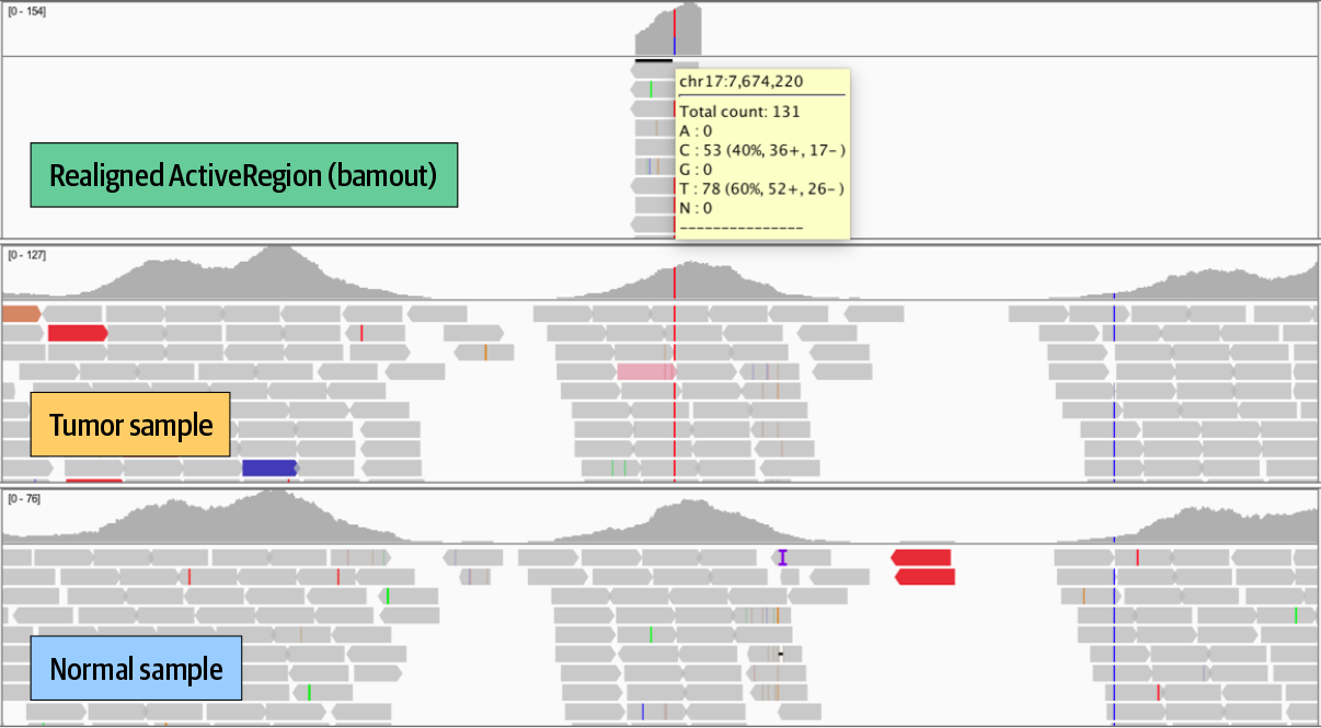
Figure 7-4. Zooming in on TP53 in IGV.
What do you think of this somatic variant call?
Annotating Predicted Functional Effects with Funcotator
Filtering somatic mutation calls can be an especially daunting task compared to their germline equivalent. It can therefore be particularly helpful to annotate the calls with predicted functional effects and their significance. For example, a stop codon in the middle of a protein coding region is likely to be more significant than a mutation in the middle of an intron. Knowing this about your calls can help you prioritize which ones you spend time investigating in depth.
To gauge functional impact, we need to know which regions of the genome code for protein sequence and which correspond to elements important to gene expression. Transcript annotation resources such as GENCODE capture such information in the standardized Gene Transfer Format (GTF). The GATK team provides a set of resources containing compiled functional annotation resources, or datasources, that are suitable for many common functional annotation needs as well as a tool called Funcotator to annotate your callset with information from these datasources. You can also create your own custom data sources. In addition, although Funcotator outputs results in VCF by default, you can make it output Mutation Annotation Format (MAF), instead, which the cancer genomics community uses extensively. See the Funcotator documentation for details on both options.
For now, though, let’s apply Funcotator to our filtered Mutect2 callset:
# gatk Funcotator \
    --data-sources-path resources/funcotator_dataSources_GATK_Workshop_20181205/ \
    --ref-version hg38 \
    -R ref/Homo_sapiens_assembly38.fasta \
    -V sandbox/m2_somatic_calls.filtered.vcf.gz \
    -O sandbox/m2_somatic_calls.funcotated.vcf.gz \
    --output-file-format VCF
This runs very quickly and produces a VCF in which our somatic callset has now been lovingly annotated based on the GENCODE functional data. Here’s a sneak peek of what the annotations look like in their natural habitat:
# zcat sandbox/m2_somatic_calls.funcotated.vcf.gz | grep -v '##' | head -3
#CHROM  POS     ID      REF     ALT     QUAL    FILTER  INFO    FORMAT  HCC1143_normal
HCC1143_tumor
chr17   1677390 .       A       T       .       weak_evidence
CONTQ=19;DP=23;ECNT=1;FUNCOTATION=[PRPF8|hg38|chr17|1677390|1677390|INTRON||SNP|A|A|T|
g.chr17:1677390A>T|ENST00000572621.5|-|||c.e13-
175T>A|||0.4463840399002494|CTGCCTCTCAAGGCCCCAGAA|PRPF8_ENST00000304992.10_INTRON];
GERMQ=32;MBQ=33,31;MFRL=301,311;MMQ=60,60;MPOS=22;NALOD=1.06;NLOD=3.01;POPAF=6.00;SEQQ
=1;STRANDQ=17;TLOD=4.22 GT:AD:AF:DP:F1R2:F2R1:SB       0/0:10,0:0.081:10:6,0:4,0:6,4,0,
0	0/1:9,2:0.229:11:5,1:3,1:6,3,2,0
chr17   2394409 .       G       T       .       PASS
CONTQ=93;DP=106;ECNT=1;FUNCOTATION=[MNT|hg38|chr17|2394409|2394409|INTRON||SNP|G|G|T|
g.chr17:2394409G>T|ENST00000575394.1|-|||c.e1-
6231C>A|||0.6209476309226932|TTCCTGACCAGCGCCGCCACC|MNT_ENST00000174618.4_INTRON];
GERMQ=93;MBQ=32,31;MFRL=148,177;MMQ=60,60;MPOS=14;NALOD=1.56;NLOD=10.52;POPAF=6.00;SEQQ
=93;STRANDQ=93;TLOD=30.05  GT:AD:AF:DP:F1R2:F2R1:SB       0/0:35,0:0.027:35:15,0:19,0:4,
31,0,0	0/1:53,13:0.206:66:23,5:29,8:13,40,4,9
Now let’s have a look at the annotations specifically for the TP53 mutation that we viewed earlier in IGV, at chr17:7674220:
# zcat sandbox/m2_somatic_calls.funcotated.vcf.gz | grep 7674220
chr17   7674220 .       C       T       .       PASS
CONTQ=93;DP=134;ECNT=1;FUNCOTATION=[TP53|hg38|chr17|7674220|7674220|MISSENSE||SNP|C|C|T|
g.chr17:7674220C>T|ENST00000269305.8|-|7|933|c.743G>A|c.(742-
744)cGg>cAg|p.R248Q|0.5660847880299252|GATGGGCCTCCGGTTCATGCC|TP53_ENST00000445888.6_MISSENSE_
p.R248Q/TP53_ENST
00000420246.6_MISSENSE_p.R248Q/TP53_ENST00000622645.4_MISSENSE_p.R209Q/
TP53_ENST00000610292.4_MISSENSE_p.R209Q/TP53_ENST00000455263.6_MISSENSE_p.R248Q/
TP53_ENST00000610538.4_MISSENSE_p.R209Q/TP53_ENST00000620739.4_MISSENSE_p.R209Q/
TP53_ENST00000619485.4_MISSENSE_p.R209Q/TP53_ENST00000510385.5_MISSENSE_p.R116Q/
TP53_ENST00000618944.4_MISSENSE_p.R89Q/TP53_ENST000005
04290.5_MISSENSE_p.R116Q/TP53_ENST00000610623.4_MISSENSE_p.R89Q/
TP53_ENST00000504937.5_MISSENSE_p.R116Q/TP53_ENST00000619186.4_MISSENSE_p.R89Q/
TP53_ENST00000359597.8_MISSENSE_p.R248Q/TP53_ENST00000413465.6_MISSENSE_p.R248Q/
TP53_ENST00000615910.4_MISSENSE_p.R237Q/TP53_ENST00000617185.4_MISSENSE_p.R248Q];
GERMQ=93;MBQ=31,32;MFRL=146,140;MMQ=60,60;MPOS=21;NALOD=1.73;NLOD=15.33;POPA
F=6.00;SEQQ=93;STRANDQ=93;TLOD=264.54      GT:AD:AF:DP:F1R2:F2R1:SB
0/0:51,0:0.018:51:22,0:29,0:36,15,0,0   0/1:0,76:0.987:76:0,38:0,38:0,0,52,24
This SNV is a C-to-T substitution that is predicted to cause an arginine-to-glutamine missense mutation. Missense mutations change the protein that is produced from the gene, which can be functionally neutral, but can also have deleterious effects. If we look at the rest of the file, out of our 124 mutation records, 21 were annotated as MISSENSE; and of these, 10 passed all filters. That information should help us prioritize what to investigate in the next stage of our analysis.
With that, we’re done with the Tumor-Normal pair analysis workflow for discovery of somatic SNVs and indels! Next, we’re going to go over the process we apply for investigating somatic copy-number alterations.
Somatic Copy-Number Alterations
So far, we’ve been looking exclusively at small variants, SNVs, and indels that are characterized based on the presence or absence of specific nucleotides compared to the reference sequence. Moving to the copy number involves a big mental (and methodological!) shift given that now we’re going to be looking at the relative amounts of sequence in the sample of interest, measured relative to itself (Figure 7-5 and Figure 7-6). In other words, we’re not actually going to measure the copy number that is physically present in the biological material. What we measure is the copy ratio, which we use as a proxy because it is a consequence of copy-number alterations (CNAs). As part of that process, we’re going to use the reference genome primarily as a coordinate system for defining segments that display CNAs.
As shown in Figure 7-5, the copy number is the absolute, integer-valued number of copies of each locus (i.e., gene or other meaningful segment of DNA). The copy ratio is the relative, real-valued ratio of the number of copies of each locus to the average ploidy.
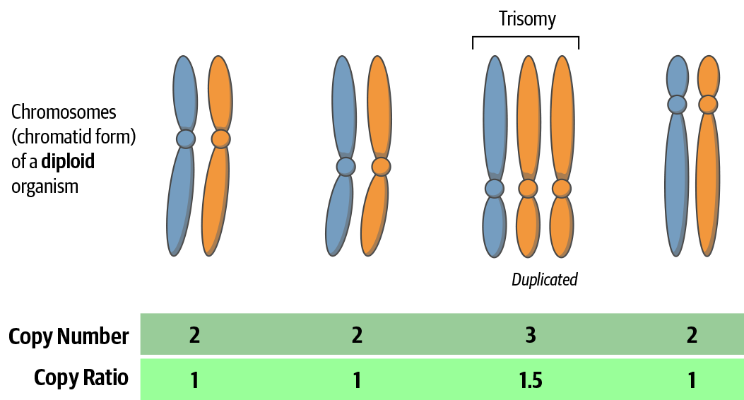
Figure 7-5. Difference between copy number and copy ratio.
Figure 7-6 shows the striking contrast in genomic composition between a normal cell line that has the expected copy number for all chromosomes (left) and a cancer cell line that has suffered multiple major CNAs (right), not to mention a variety of structural alterations. For the normal cell line in this figure (and indeed, most healthy human cells), any given chromsome’s copy number is 2 and its copy ratio is 1. Meanwhile, in the cancer cell line, there is a lot of variation between chromosomes; for example, it looks like the copy number for chromosome 7 is 5, whereas for chromosome 12 it is 3, and we can’t really guess their copy ratio because the alterations are so extensive that we don’t have a good sense of the average ploidy of this genome.

Figure 7-6. Spectral karyotyping paints each chromosome pair with a color, showing various chromosomal segments that are amplified or missing (colors in left and right panels are not expected to match).
The good news is that copy-number analysis is less sensitive than short variant analysis to some of the challenges that we enumerated earlier because we don’t care as much about exact sequence. However, it is more sensitive to technical biases that affect the evenness of sequence coverage distribution. The consequence of these two points for the analysis design is that it is less important to have a matched normal available, whereas it is even more important to have a PoN composed of normals that have a closely matching technical profile. Note, however, that the copy-number PoN is completely different from the PoN used for short variant analysis. We go over the specifics in the next section.
Overview of the Tumor-Only Analysis Workflow
The standard workflow for somatic copy-number analysis involves four main steps (Figure 7-7). First, we collect proportional coverage statistics for the case sample as well as any normals that will be used for the PoN. Setting the case sample aside for a moment, we create a copy-number PoN that captures the amount of systematic skew in coverage observed across the exome or genome. Then, we use that information to normalize the coverage data we collected for the case sample, which eliminates technical noise and reveals actual copy ratio differences in the data. Finally, we run a segmentation algorithm that identifies contiguous segments of sequence that presents the same copy ratio, and emit CNA calls for those segments whose copy ratio diverges significantly from the mean. Optionally, we can produce plots to visualize the data at several stages, which is helpful for interpretation.
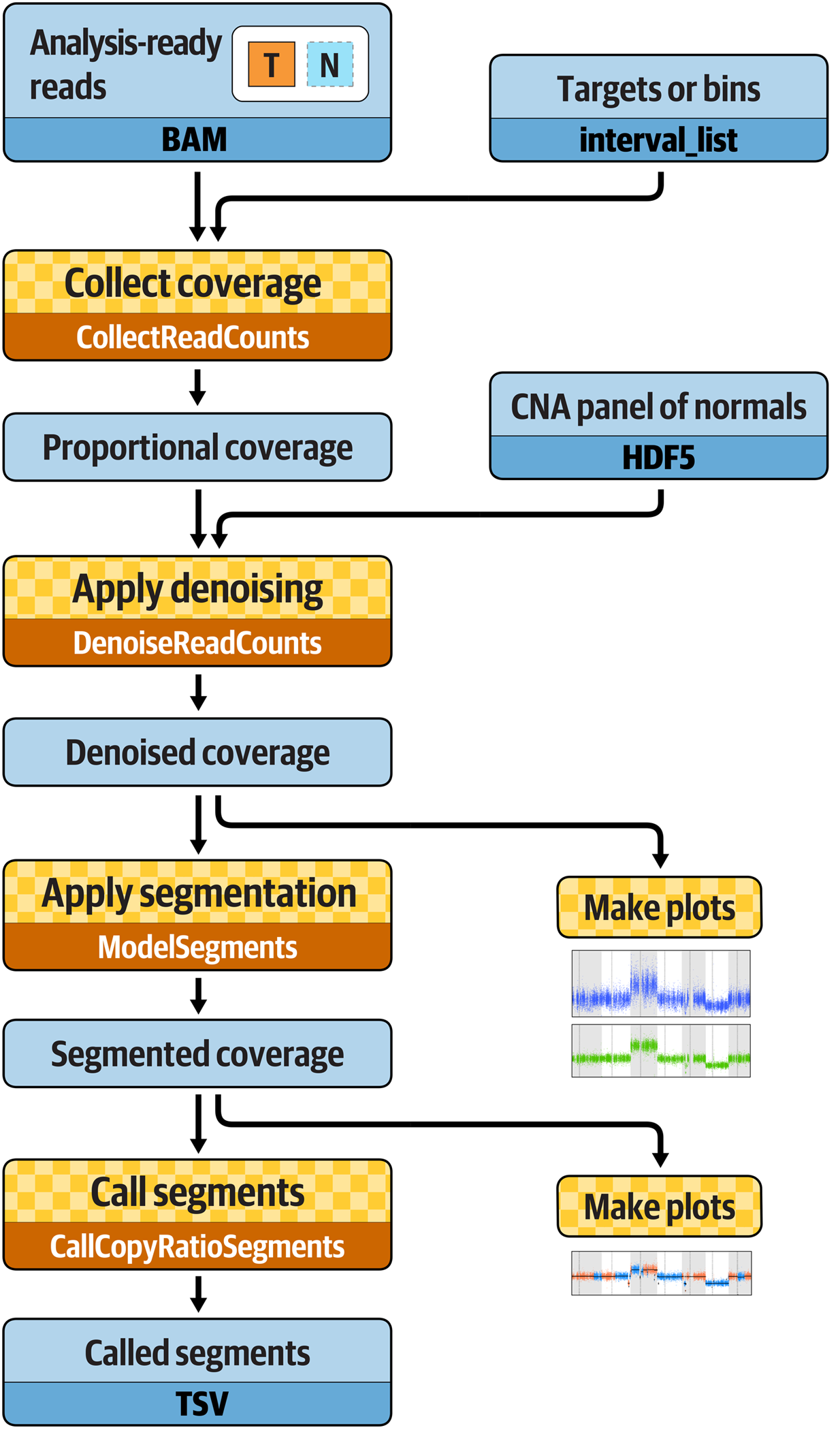
Figure 7-7. Best Practices workflow for somatic copy-number alteration discovery.
Again, you’re going to do this work from within the GATK container on your VM, so make sure everything is turned on and you’re in the /home/book/data/somatic directory. The exercises in this section use the same reference genome and some of the same resource files as the first section, and we’re going to use the same sandbox for writing outputs.
Collecting Coverage Counts
We count read depth, or coverage, over a series of intervals. Here we use exome capture targets because we’re analyzing exomes, but if we were analyzing whole genomes, we would switch to using bins of arbitrary length. For exomes, we take the interval list that corresponds to the capture targets (specific to every manufacturer’s exome prep kit) and first add some padding:
# gatk PreprocessIntervals \
    -R ref/Homo_sapiens_assembly38.fasta \
    -L resources/targets_chr17.interval_list \
    -O sandbox/targets_chr17.preprocessed.interval_list \
    --padding 250 \
    --bin-length 0 \
    --interval-merging-rule OVERLAPPING_ONLY
In this command, the --interval-merging-rule argument controls whether the GATK engine should merge adjacent intervals for processing. In some contexts, it makes sense to merge them, but in this context, we prefer to keep them separate in order to have more fine-grained resolution, and we’ll merge only intervals that actually overlap.
Note
If we wanted to generate an intervals list for whole genome data, we would run the same tool but without the targets file, and with the --bin-length argument set to the length of bin we want to use (set to 100 bases by default).
When we have the analysis-ready intervals list, we can run the read count collection tool, which operates by counting how many reads start within each interval. By default, the tool writes data in HDF5 format, which is handled more efficiently by downstream tools, but here we change the output format to tab-separated values (TSV) because it is easier to peek into:
# gatk CollectReadCounts \
    -I bams/tumor.bam \
    -L sandbox/targets_chr17.preprocessed.interval_list \
    -R ref/Homo_sapiens_assembly38.fasta \
    -O sandbox/tumor.counts.tsv \
    --format TSV \
    -imr OVERLAPPING_ONLY
The output file includes a header that recapitulates the sequence dictionary, followed by a table of counts for each target:
# head -5 sandbox/tumor.counts.tsv
@HD     VN:1.6
@SQ     SN:chr1 LN:248956422
@SQ     SN:chr2 LN:242193529
@SQ     SN:chr3 LN:198295559
@SQ     SN:chr4 LN:190214555
Annoyingly, the sequence dictionary for the hg38 reference build is extremely long because of the presence of all the ALT contigs (explained in the genomics primer in Chapter 2). So, to peek into our file, it’s better to use tail instead of head:
# tail -5 sandbox/tumor.counts.tsv
chr17   83051485        83052048        1
chr17   83079564        83080237        0
chr17   83084686        83085575        1010
chr17   83092915        83093478        118
chr17   83094004        83094827        484
Ah, that’s more helpful, isn’t it? The first column is the chromosome or contig, the second and third are the start and stop of the target region we’re looking at, and the fourth is the count of reads overlapping the target. Figure 7-8 provides an example of what this looks like visualized.
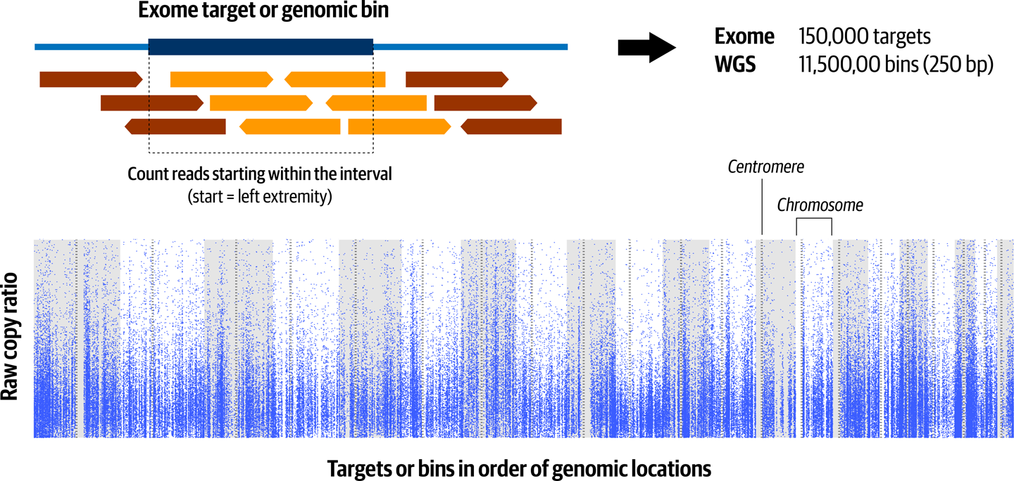
Figure 7-8. Read counts in each genomic target or bin form the basis for estimating segmented copy ratio, and each dot is the value for a single target or bin.
Each dot in the figure represents one of the intervals for which we collected coverage, arranged in the order of their position on the genome. The gray and white stripes in the background represent alternating chromosomes, and the dotted lines represent the position of their centromeres. Notice how the dots form a wavy smear because of the huge variability in the amount of coverage present from one to the next. At this point, it’s impossible to identify any CNAs with any kind of confidence.
Creating a Somatic CNA PoN
As we discussed in Chapter 2, a lot of technical variability affects the sequencing process, and some of it is fairly systematic—some regions will produce more sequence data than others, mainly because of chemistry. We can establish a baseline of what normal variability looks like by using an algorithm called singular value decomposition, which is conceptually similar to principal component analysis and aims to capture systematic noise from a panel of normals that were sequenced and processed the same way. The minimum number of samples in a CNA PoN should be at least 10 normal samples for the tools to work properly, but the Best Practices recommendation is to use 40 or more normal samples if possible.
Creating the PoN is a lot of work, so we provide one for you made from 40 samples from the 1000 Genomes Project. Each of the 40 samples was run individually through the CollectReadCounts tool, as described earlier (but leaving the default output format set to HDF5; hence, the .hdf5 extension in the command line, shown in the next code snippet). Then the panel was created by running the command that follows on all the read count files. To be clear, we’re just showing this as an example, so don’t try to run it; it won’t work with the data we’ve provided for the book. for the book; we’re just showing it as an example.
gatk CreateReadCountPanelOfNormals \
    -I file1_clean.counts.hdf5 \
    …
    -I file40_clean.counts.hdf5 \
    -O cnaponC.pon.hdf5
The PoN produced by this command is completely different from the one we created for the short variant section earlier in this chapter. For the short variants pipeline, the PoN was just a kind of VCF file with annotated variant calls. In this case, however, the file produced by aggregating the read count data from the 40 normals is not meaningfully readable by the naked eye.
Applying Denoising
With our sample read counts in hand and the PoN ready to go, we have everything we need to run the most important step in this workflow: denoising the case sample read counts:
# gatk DenoiseReadCounts \
    -I cna_inputs/hcc1143_T_clean.counts.hdf5 \
    --count-panel-of-normals cna_inputs/cnaponC.pon.hdf5 \
    --standardized-copy-ratios sandbox/hcc1143_T_clean.standardizedCR.tsv \
    --denoised-copy-ratios sandbox/hcc1143_T_clean.denoisedCR.tsv
Even though we’re running only a single command, internally the tool is performing two successive data transformations. First, it standardizes the read counts by the median counts recorded in the PoN, which involves a base-2 log transformation and normalization of the distribution to center around one, to produce copy ratios. Then, it applies the denoising algorithm to these standardized copy ratios using the principal components of the PoN.
Note
You can tune the denoising tool to be more or less aggressive by adjusting the --number-of-eigensamples parameter, which affects the resolution of results; that is, how smooth the resulting segments will be. Using a larger number will produce a higher level of denoising but can reduce the sensitivity of the analysis.
Again, the output files are not really human readable, so let’s plot their contents to get a sense of what the data shows at this point:
# gatk PlotDenoisedCopyRatios \
    --sequence-dictionary ref/Homo_sapiens_assembly38.dict \
    --standardized-copy-ratios sandbox/hcc1143_T_clean.standardizedCR.tsv \
    --denoised-copy-ratios sandbox/hcc1143_T_clean.denoisedCR.tsv \
    --minimum-contig-length 46709983 \
    --output sandbox/cna_plots \
    --output-prefix hcc1143_T_clean
The resulting plot includes both the standardized copy ratios produced by the first internal step and the final denoised copy ratios (Figure 7-9).
You can use gsutil to copy the output plots from your VM to your Google bucket and then view them (or download them) from the GCP console. If you need a refresher on this, see Chapter 4. The following is done from your VM (which has the gsutil tool installed and configured in Chapter 4) rather than the Docker container you’ve run the gatk commands in, and uploads to the bucket that you specify (my-bucket) in this example:
$ export BUCKET="gs://my-bucket"
$ gsutil -m cp -R sandbox/cna_plots $BUCKET/somatic-sandbox/
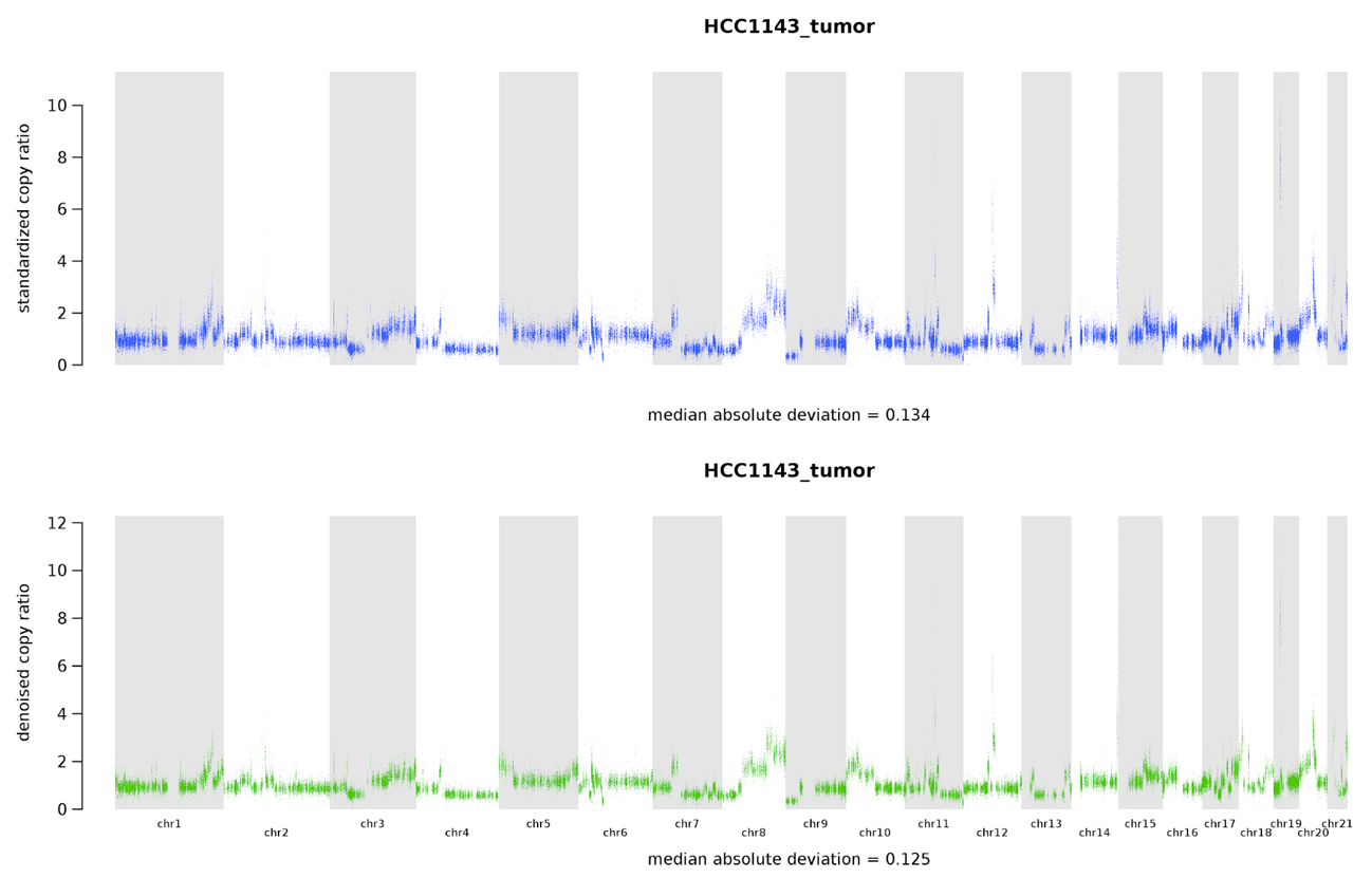
Figure 7-9. Copy-number alteration analysis plots showing the standardized copy ratios after the first step of denoising (top) and the fully denoised copy ratios after the second round (bottom).
It can be difficult to see very clearly in the book version of these images, but if you zoom in on the plots you generated yourself, you should be able to see that the range of values in the second-round image is tighter than in the first round, which shows the improvement from one step to the next. In any case, we can agree that these show much better resolution compared to the raw read counts shown in Figure 7-8, and we can already discern some probable CNAs.
Performing Segmentation and Call CNAs
Now that we have our lovingly denoised copy ratios, all we need to do is identify exactly which regions demonstrate evidence of CNA. To do that, we’re going to group neighboring intervals that have similar copy ratios into segments. Then, we should be able to determine which segments have an overall copy ratio that supports the presence of an amplification or deletion relative to the rest.
We do this using the ModelSegments tool, which uses a Gaussian-kernel binary-segmentation algorithm to perform multidimensional kernel segmentation.
# gatk ModelSegments \
    --denoised-copy-ratios sandbox/hcc1143_T_clean.denoisedCR.tsv \
    --output sandbox  \
    --output-prefix hcc1143_T_clean
As for the previous plots, the easiest way to view these is to transfer them to your Google bucket and open (or download) them from the GCP console. This command produces multiple files, so the output name we provide is simply the name that we want to give to the new directory that will contain them. Again, the outputs are not particularly user friendly, so we’re going to make some plots to visualize the results. We provide the plotting tool with the denoised copy ratios (from DenoiseReadCounts), the segments (from ModelSegments), and the reference sequence dictionary:
# gatk PlotModeledSegments \
    --denoised-copy-ratios sandbox/hcc1143_T_clean.denoisedCR.tsv \
    --segments sandbox/hcc1143_T_clean.modelFinal.seg \
    --sequence-dictionary ref/Homo_sapiens_assembly38.dict \
    --minimum-contig-length 46709983 \
    --output sandbox/cna_plots \
    --output-prefix hcc1143_T_clean
Figure 7-10 shows the segments identified by the PlotModelSegments tool. The dots representing targets or bins on alternate segments are colored in either blue and orange, whereas segment medians are drawn in black. Most segments have a copy ratio of approximately 1, which constitutes the baseline. Against that backdrop, we can observe multiple amplifications and deletions of different sizes and different copy ratios. You might notice that most of these don’t correspond to the numbers that you would expect if you had, for example, four copies instead of two for a given segment. That is because some of the CNAs occur in subclonal populations, meaning that only part of the sampled tissue is affected. As a result, the effect is diluted and you might see a copy ratio of 1.8 instead of 2.

Figure 7-10. Plot of segments modeled based on denoised copy ratios.
More generally, it seems like a lot is going on in this sample; in fact, we can look in the segmentation file in the output directory and see that we’ve predicted 235 segments for this sample. This isn’t typical of regular tumor samples, although some can be pretty messed up; what’s going on here is that we’re looking at a sample taken from a cell line. Cancer cell lines are convenient for teaching and testing software because the data can easily be made open access, but biologically they tend to have accumulated very high numbers of alterations. So this represents an extreme situation. On the bright side, most samples that you’ll encounter in the real world are likely to be cleaner (and easier to interpret) than this. So you have something to look forward to!
That being said, the software can still help us get a bit more clarity even on a messy sample like this. We can get final CNA calls—that is, a determination of which segments we can consider to have significant evidence of amplification or deletion—by running the last tool in this workflow, as follows:
# gatk CallCopyRatioSegments \
    -I sandbox/hcc1143_T_clean.cr.seg \
    -O sandbox/hcc1143_T_clean.called.seg
This tool adds a column to the segmented copy-ratio .cr.seg file from ModelSegments, marking amplifications (+), deletions (-), and neutral segments (0):
# tail -5 sandbox/hcc1143_T_clean.called.seg
chrX    118974529       139746109       864     0.475183        +
chrX    139749773       139965748       28      -0.925385       -
chrX    140503468       153058699       277     -0.366860       -
chrX    153182138       153580550       47      0.658197        +
chrX    153588113       156010661       544     0.075279        0
And there you have it; this shows you the output of the somatic copy-number workflow. If we look at the full progression, you can see that we went from raw coverage counts all the way to having identified specific regions of deletion or amplification, as illustrated in Figure 7-11 (using different data and only a subset of chromosomes).
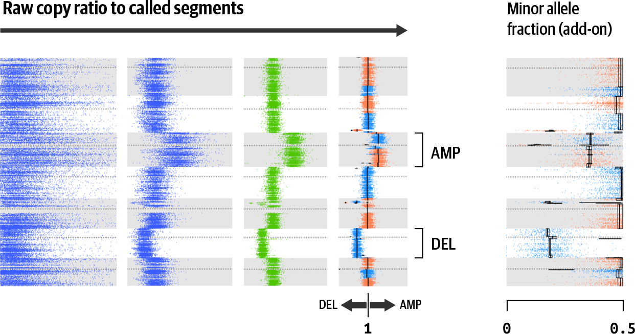
Figure 7-11. Full progression from raw data to results.
Copy ratio counts in Figure 7-11 are calculated and processed as shown in previous figures, rotated 90° to the right. The leftmost panel shows raw copy ratio counts calculated per target or genomic bin. The second and third panels show standardized and denoised counts, respectively. The fourth panel shows segmentation and calling results, including one whole chromosome amplification (AMP) and one deletion (DEL). The rightmost panel shows a minor allele fraction calculated using the procedure outlines in the next section.
Ironically, these results don’t include an actual copy number, just the boundaries of each segment, its copy ratio, and the final call. To get the copy number, you will need to do some additional work that is beyond the scope of this chapter. See the documentation for more information and next steps.
Additional Analysis Options
We’ve just covered the standard workflow that is most commonly used for performing copy-number analysis with GATK tools. This involved collecting coverage counts, using a PoN to apply denoising, and performing segmentation in order to model and finally call copy-number–altered segments on the tumor case sample. However, you can apply two additional options to further beef up the quality of the results.
Tumor-Normal pair analysis
The Tumor-only workflow gets you decent, usable results for somatic CNA discovery. But if you have a matched normal available, you can gain additional benefits! For one thing, you can run the workflow, as described earlier on the normal sample, which is helpful for understanding the baseline that you’re working with. In many cases, having the matched normal can also help the denoising process.
Feel free to run through the commands on your own. In the final segmentation results, notice the probable CNAs on chromosome 2 and chromosome 6. This matched normal is itself from a cell line, albeit derived from healthy tissue instead of a tumor. It’s not uncommon to see some background alterations occur even in normal tissue when it’s been propagated as a cell line.
Note
This concludes the exercises for this chapter, so once again, remember to stop your VM if you’re taking a break before moving on to the next chapter.
Allelic copy ratio analysis
So far, we’ve used only read coverage as evidence for CNAs, but we can also include allelic copy ratio: the copy ratio for different alleles at sites with heterozygous SNVs. This can reveal interesting things about the heterozygosity of our case sample, which can have important biological consequences—especially when there is a loss of heterozygosity.
We can detect imbalances in the heterozygosity of segments by looking at the allelic counts (i.e., the read counts for different alleles at each site) in the case sample at sites that are commonly variant in the population. For a diploid organism, we expect to see any heterozygous SNV manifest as two different alleles present in equal proportions. Suppose that we have an A/T variant; we expect to see approximately 50% A and 50% T in the sequence reads (give or take some technical variability). We can detect those sites on the fly when we’re counting the reads in the first step of the workflow. Then, we can use those sites as markers; if we look at those sites in the tumor and find that their allelic ratios are significantly skewed, that gives us additional information about the degree of CNA that affects the segments of which these sites are part.
If you’re interested in exploring this additional analysis mode, have a look at the somatic copy-number documentation on the GATK website.
Wrap-Up and Next Steps
Well then, between the germline workflow and these two somatic analysis workflows, we’ve already run a lot of genomics commands. So, does that mean we’re ready to run full-scale genomic analyses?
Hah, no. At this point you can run individual tools one by one—which is going to be useful at various stages of your work, especially for initial testing/evaluation as well as troubleshooting failures—but you also know that the variant discovery Best Practices are composed of multiple tasks involving various tools. Trust us, you don’t want to be running each task manually for each sample or set of samples that you need to process. You’re going to want to chain these tasks into scripts that automate the bulk of the work to cut down on the mindless tedium as well as to reduce the chance of human error. So in Chapter 8, we show you how to write workflow scripts using WDL, which automates calling each step in the overall analysis pipeline. Then, we run them using a workflow management system called Cromwell that is equally comfortable running on your laptop, cluster, or cloud platform.