Chapter 6. GATK Best Practices for Germline Short Variant Discovery

By now, we’ve introduced all of the major concepts and tools, and we’ve walked through a few examples, calling variants with the GATK HaplotypeCaller and exploring its output. It’s time to turn up the dial on the analytical complexity and take a closer look at the three GATK Best Practices workflows.

In this chapter, we explore the most widely used variant discovery pipeline in the genomics community: the GATK Best Practices for germline short variant discovery in multiple samples, which is designed to take advantage of the benefits of including more data in the analysis process. We begin with an overview of the initial data processing and quality control steps that are necessary to render the data suitable for analysis. Then, we’ll dive into the details of the joint calling workflow. In the final part of this chapter, we also cover the highlights of an alternate workflow that supports single-sample calling for use when multisample calling is not an option, as in the context of clinical analysis.

Data Preprocessing

As we discussed in the genomics primer, the data produced by the sequencing process is not immediately suitable for performing variant discovery analysis. We need to preprocess that raw output to transform it into the appropriate format and clean up some technical issues. In this section, we outline the key steps and their rationale. However, we don’t run through the entire preprocessing workflow in detail, nor do we perform any hands-on exercises. At this point, it is becoming increasingly more common for the sequencing service providers to perform this as an extension of the data-generation process, and rarer for researchers to need to do this work themselves, so we would rather focus on later stages for which a deeper exploration will likely be of more practical utility to you.

As Figure 6-1 summarizes, the preprocessing workflow consists of three main steps: mapping reads to the genome reference, marking duplicates, and recalibrating base quality scores. In practice, a full pipeline implementation will typically involve some additional “plumbing” steps. For full details, we recommend consulting the Broad Institute’s reference implementations for whole-genome processing and for exome processing.

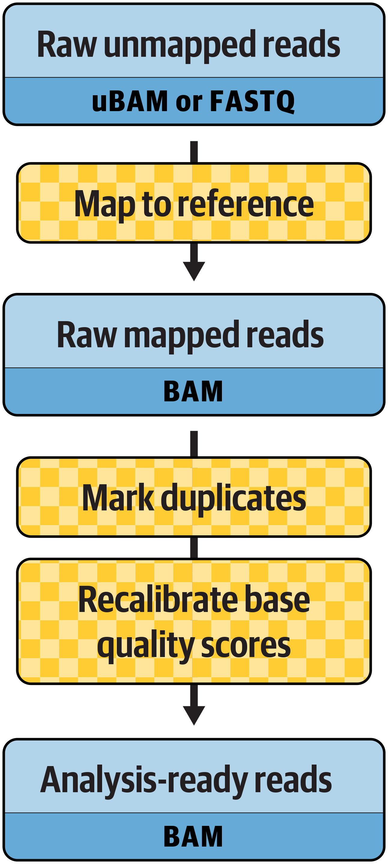
Figure 6-1. The main steps in the preprocessing workflow.

Note

Old versions of the preprocessing included an additional step called Indel Realignment, which corrected for alignment errors in the mapping step. That step is no longer needed if you use a graph-based variant caller for calling short variants, as discussed in the section on the HaplotypeCaller tool in Chapter 5.

The preprocessing workflow is designed to operate independently on data from individual samples. The per-sample data is usually further divided into distinct subsets called read groups. As a reminder, read groups correspond to the intersection of DNA libraries and flowcell lanes generated through multiplexing, as explained in Chapter 2.

Some sequence providers collapse multiple read groups into a single FASTQ file, with the very unfortunate consequence that you lose the ability to distinguish read groups. This is bad for two reasons. First, it forces you to process a large monolithic file through the mapping step, which is going to be a performance bottleneck in the pipeline, requiring you to do extra work in the workflow implementation. Second, it hamstrings the base recalibration algorithm, which prefers to operate per read group for reasons that we get to shortly.

In contrast, keeping read group data in separate files in the initial stages allows us to process those read groups independently through the mapping step, which is computationally more favorable. We’ll bring those read groups together into a single file for each step when we run the duplicate marking step.

We apply the same preprocessing steps for almost all sequencing data that are destined for variant calling, regardless of the type of variants we’re looking for, with a few exceptions. For example, we use a different mapper for RNAseq in order to deal with intronic regions appropriately. Fortunately, if we’re looking for multiple types of variants in the same data, we need to do this preprocessing only once; the resulting BAM file is suitable for input to all the GATK Best Practices variant discovery workflows.

Mapping Reads to the Genome Reference

Because the sequencer spits out individual reads without any indication of where each read belongs in the genome, the first essential step in the workflow is to map reads to the reference genome and assign an exact position for each base in the read. As a result, mapping is sometimes called alignment instead, but we prefer to use the term mapping because it is more reflective of the primary value we draw from this step: identifying where the read belongs in the genome. As you’ll see later in this chapter, we don’t completely trust the fine local alignment provided by the mapper. It’s a bit like the GPS navigation system in a car: you can usually trust it to get you to your desired street location, but you wouldn’t trust it to parallel park the car along the curb.

Many mappers are available, and in theory you could choose to use whatever mapper conforms to the main requirements of the GATK Best Practices guidelines in terms of inputs and outputs, and produces high-quality results. However, in practice, the GATK development team currently recommends using a specific tool, bwa mem, in order for your data to be compatible for cross-analysis with other datasets, for the reasons we outlined in “Functional Equivalence Pipeline Specification”. It is possible that this recommendation might change in the future.

Here’s an example of a simple command used to map sequence data with bwa mem on an interleaved FASTQ file, which contains both forward and reverse reads for each pair, sorted by query name (you don’t need to run this on your VM; it’s just for illustration):

bwa mem -M -t 7 -p reference.fasta unmapped_reads.fq > mapped_reads.sam

This command takes the FASTQ file and produces an aligned SAM format file containing the mapped read data. Each read record now includes read mapping position and alignment information as well as additional metadata. The reads are sorted in the same order in the output as they were in the input FASTQ file.

Note

In previous chapters, you’ve seen us use a prompt with $ to indicate commands to run on your VM and a prompt with # to indicate a command to run inside a Docker container. When we show you sample commands that don’t start with $ or #, these commands are just for your reference, and we don’t intend you to run them directly.

In the Broad Institute’s production implementation of the GATK Best Practices, the unmapped read data is stored in unmapped BAM files instead of FASTQ. As we noted in Chapter 2, read data can be stored in BAM format without any mapping information. The advantage of using this format is that it allows us to store metadata associated with the sequence (such as read group) within the same file, rather than relying on additional files for that purpose. This simplifies data management operations and reduces the chance that metadata might be lost or associated with the wrong data. This does, however, add a few steps to the pipeline implementation, which you can see in action in the reference implementation workflow.

When processing sample data that is distributed into multiple read groups, we run this step individually per read group, which speeds up processing if you are able to run the read group data in parallel on multiple machines. In addition, because mapping operates on each read independently of any others, it can be further parallelized at the CPU level. The example command we provided specifies that the process should use seven threads (-t 7) to maximize efficiency on a common type of machine with eight cores available. However, you can parallelize this step to a much higher degree if you have specialized hardware available. That is how computing platforms that offer accelerated genomics pipelines such as DRAGEN can derive major speed gains from boosting parallelization of the mapping step through specialized hardware such as FPGAs (see Chapter 3 for an explanation of these terms).

As soon as we have generated the mapped data in BAM (or equivalent) format, we could technically go straight to the variant calling step. However, we know there are some technical sources of error that we can deal with at this stage: the presence of duplicate reads and of systematic biases in the assignment of base quality scores. Let’s apply the recommended mitigation strategies before we try to call variants, as prescribed by the GATK Best Practices.

Marking Duplicates

Duplicate reads are reads that are derived from the same original physical fragment in the DNA library, originating at two different stages of the preparation and sequencing processes. During library preparation itself, if the protocol involves a PCR amplification step, each cycle of PCR will produce increasing amounts of duplicate fragments. This used to be necessary to generate enough starting material for the sequencing process, but recent improvements in the technology have made PCR amplification unnecessary in most modern protocols, so that source of duplicates has been significantly reduced. The other major source of duplicates, during the sequencing process, is caused by various optical confusions—for example, when a single DNA cluster on the Illumina flowcell is called as two distinct clusters and treated as two different reads.

We consider these duplicates to be nonindependent observations, so we want to take only one representative of each group into account in downstream analyses. To that end, we’ll use a Picard tool called MarkDuplicates that identifies groups of duplicates, scores them to determine which one has the highest sequence quality, and marks all the other ones with a tag that allows downstream tools (such as variant callers) to ignore them, as illustrated in Figure 6-2.

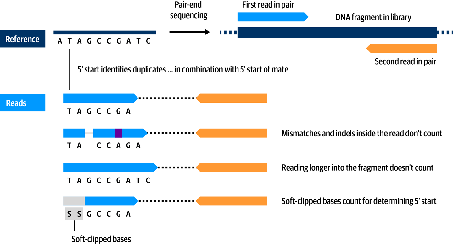
Figure 6-2. Reads marked as duplicates because they originated from the same DNA fragment in the library.

This processing step is performed per sample across read groups, if applicable. When processing sample data that is distributed into multiple read groups, this is the step where we consolidate the read group data files into a single per-sample file by feeding all read group input files to the MarkDuplicates tool. Conveniently, the tool will produce a single sorted file containing the data from all the read groups. This means that we can avoid running the consolidation in a separate step. Here’s an example showing what the command looks like when run on data from three read groups belonging to the same sample:

gatk MarkDuplicates \
    -R reference.fasta \
    -I mapped_reads_rg1.bam \
    -I mapped_reads_rg2.bam \
    -I mapped_reads_rg3.bam \
    -O sample_markdups.bam

The BAM file output by the duplicate marking step still contains all of the same reads as before, but now some of them have been tagged, and downstream tools can choose to use them or ignore them, depending on what is appropriate for their purposes, as shown in Figure 6-3.

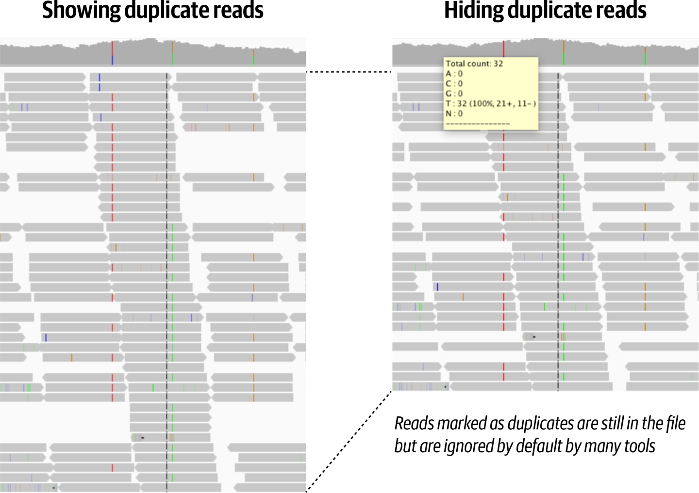
Figure 6-3. The effect of duplicate marking visualized in Integrated Genome Viewer.

This step has long constituted a major bottleneck in traditional pipelines because it involves making a large number of comparisons between all of the read pairs belonging to the sample, across all of its read groups. It also requires a sorting operation because it operates across all reads belonging to the sample. To address this issue, the GATK team ported MarkDuplicates in the GATK4 framework using Spark to speed up its operation, which yields major performance gains when using multicore CPUs for processing. The MarkDuplicatesSpark tool has not yet been integrated into the reference implementation of the Best Practices pipeline, but that should happen in the near future.

Recalibrating Base Quality Scores

The final processing step we need to apply to our data aims to detect and correct for patterns of systematic errors in the base quality scores, which you’ll recall are the confidence scores emitted by the sequencer for each base. Base quality scores play an important role in weighing the evidence for or against possible variant alleles during the variant discovery process for short variants, so it’s important to correct any systematic bias observed in the data. Such biases can originate from biochemical processes during library preparation and sequencing, from manufacturing defects in the flowcell chips, or instrumentation defects in the sequencer.

Base Quality Score Recalibration (BQSR) involves collecting covariate statistics from all base calls in the dataset, building a model from those statistics, and applying base quality adjustments to the dataset based on the resulting model.

Figure 6-4 shows two plots that help us understand the effect of BQSR. In panel A, we’re comparing the base qualities reported by the instrument (Reported Quality) against the base qualities that we derive from gathering all the observations with the same reported quality and seeing how many errors there are (Empirical Quality). For example, before applying the BQSR correction to the data (Original series, pink/gray), we find that a base with a quality of 30 according to the instrument should in fact be given a quality of 25, according to the quality assessed by counting mismatches in this group. This tells us that the sequencer was overly confident of its own accuracy for that subset of data, and indeed we observe that this is the case for most of the bases in this particular dataset, although there are a few bins where this trend is reversed. After applying the BQSR correction, if we run the modeling procedure again on the recalibrated data (Recalibrated series, blue/black), all of the dots align on the diagonal, which tells us that there is no longer a gap between the qualities assigned to the bases and the observed quality.

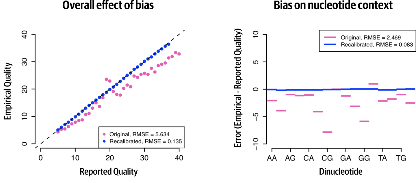
Figure 6-4. Visualizing the effect of BQSR.

Note that panel A in Figure 6-4 shows overall effect, which is based on calculations from multiple covariates. In panel B, we’re looking at one of those covariates, the dinucleotide context. This takes into account the sequence context of each base (specifically, the two bases before the base of interest), which we know can affect the accuracy of sequencing. This plot shows the average error in the base quality assignment for each of the possible dinucleotides (note that the axis legend does not show all labels; use the order A, C, G, T to identify the missing labels), where Error is defined as the difference between the quality estimated by the model (Empirical) and the quality reported by the instrument (Reported). Negative values mean that the instrument was overconfident; for example, we can say based on this plot that in this dataset, a base called after CG typically had a quality score that was inflated by ~7.5 before recalibration compared to what it should have been. After recalibration, the Error goes to zero for all bins, which means there is no longer a difference between the assigned base qualities and those calculated by modeling.

The patterns of base quality biases that we find in the data are specific to each library and flowcell, so they must be modeled anew every time; it is not possible to create a model on one dataset and apply it subsequently to other data. Here is an example command for building the model:

gatk BaseRecalibrator \
    -R reference.fasta \
    -I sample_markdups.bam \
    --known-sites known_variation.vcf \
    -O recal_data.table

This command takes the reference genome (reference.fasta) and the BAM file containing the mapped read data that has already been processed through duplicate marking (sample_markdups.bam) as well as a VCF file of variants that have been previously reported for the organism of interest (known_variation.vcf). The latter plays an important role in the recalibration model; the algorithm uses the known sites to mask out positions that it should not use in building the model. For a complete explanation of why and how this works, see the BQSR method documentation. The output of the command is a text file containing recalibration tables produced by the modeling process, which we then use to apply the model to the data. Here is an example command for applying the recalibration:

gatk ApplyBQSR \
    -R reference.fasta \
    -I sample_markdups.bam \
    --bqsr-recal-file recal_data.table \
    -O sample_markdups_recal.bam

This produces the final output (sample_markdups_recal.bam), a BAM file containing the read data with recalibrated base qualities that is ready for analysis.

This processing step is performed per sample, but the algorithm itself will differentiate between read groups because many of the biases it tracks are read group specific. The initial statistics collection can be parallelized by scattering across genomic coordinates, typically by chromosome or batches of chromosomes, but this can be broken down further to boost throughput if needed. Gathering per-region statistics into a single genome-wide model of covariation cannot be parallelized, but it is computationally trivial and therefore not a bottleneck. The final application of recalibration rules is best parallelized in the same way as the initial statistics collection, over genomic regions, then followed by a final file merge operation to produce a single analysis-ready file per sample.

Joint Discovery Analysis

Finally, the real fun begins! We’re going to call variants on a cohort of multiple people. But before we get into the weeds of how it works, let’s take a few minutes to talk about why we do it this way.

When it comes to understanding germline variation, a single person’s genome is rarely useful in isolation. Most research questions in this area will benefit from looking at data from multiple people, whether it’s a small number, as in the case of the investigation of disease inheritance from parents to their children, or a much larger number, as in the case of population genetics. So, from a scientific standpoint, we’re usually going to want to analyze multiple samples together. In addition, there are technical advantages to grouping data from multiple samples, mostly related to statistical power and compensation for technical noise.

Overview of the Joint Calling Workflow

In the early days of variant discovery, multisample analysis was done by running variant calling on each sample independently and then combining the resulting lists of variants. This approach had several weaknesses, including that it didn’t account for the difference between “no variant call because no variation” versus “no variant call because no data.” Joint analysis solves this problem because it takes only one sample with a variant of interest for a call to be made at the corresponding site across all samples. The output will then contain detailed genotyping information for all samples, allowing us to make the necessary distinctions, as demonstrated in Figure 6-5.

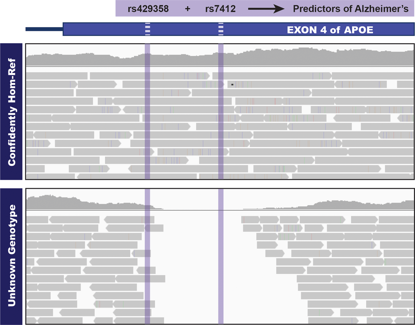
Figure 6-5. Sites that would be omitted from the VCF in a single-sample callset.

The other big advantage of joint analysis is that it allows us to boost the statistical power of the variant calling calculations by increasing the amount of data that we can take into account. This comes into play in two places: at the initial stage of calculating the confidence score of a particular variant call, and a little later, at the stage of filtering variants. The fundamental principle at play here is that when we don’t have much data to work with, we are more vulnerable to technical artifacts. For example, consider the first sample shown in Figure 6-6. We have only a handful of reads covering a particular site in that sample, and we see only one or two reads that carry what looks like a variant allele, so we’re going to be very skeptical because that could easily be a library preparation artifact or a sequencing error. We might emit a variant call, but with a very low score that is likely to get it thrown out in filtering. However, when we look at data from multiple samples, we find that we see the same potential variant allele in another sample, so we’ll be more inclined to believe there is real variation here, and we’ll give the variant a better score.

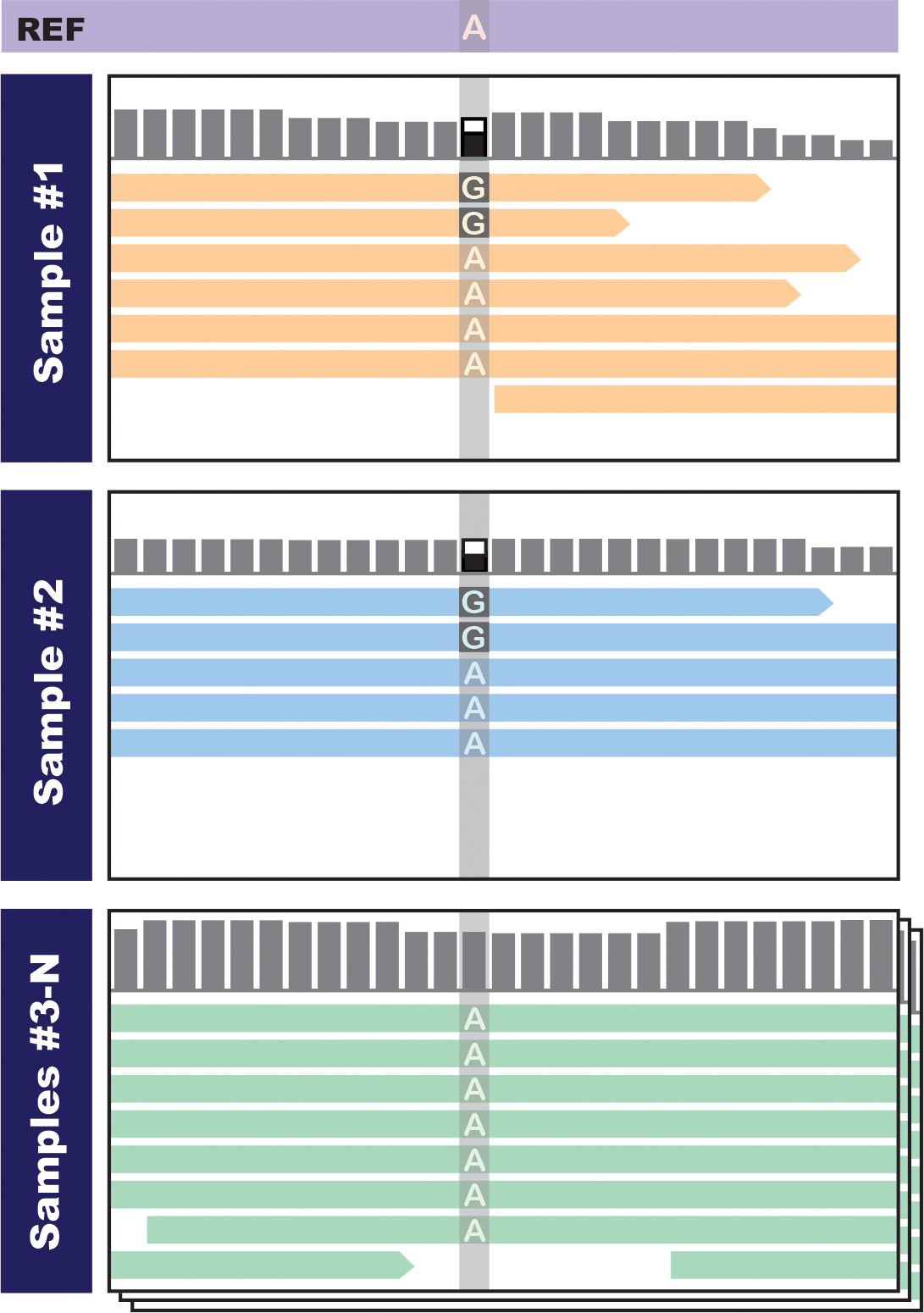
Figure 6-6. Seeing concordant evidence in multiple samples boosts our confidence that there is real variation.

Note

Boosting confidence when we see a variant in multiple samples does not mean we penalize those that show up in only one sample in a cohort, which are called singletons. The joint calling algorithm is designed to avoid penalizing singletons, so a singleton that is well supported by read data will still be called confidently.

In addition to this signal-boosting effect, which acts at the stage of calculating confidence scores, we also see important benefits later on during filtering. Having data from many samples compensates for fluctuations in data quality, reduces the effect of extreme outliers, and stabilizes the distribution of variant context annotations, a type of metadata collected during the variant calling process that we discuss in more detail in the filtering section. The benefits of joint calling for filtering are especially obvious in cohorts of up to a few hundred samples; then the gains begin to taper off, providing diminishing returns as you keep adding more samples. You can read more about this pattern in the HaplotypeCaller preprint.

So how does it work? In earlier versions of the variant discovery phase, you had to run the variant caller directly on multiple per-sample BAM files. However, that scaled very poorly with the number of samples, posing unacceptable limits on the size of the study cohorts that could be analyzed in that way. In addition, it was not possible to add samples incrementally to a study; you had to redo all variant calling work when you added new samples. This is called the N + 1 problem: imagine you’ve analyzed a cohort of N samples at considerable expense of time and money, and then you add one more sample and need to redo all that work (Figure 6-7). That’s a big problem.

Figure 6-7. Traditional multisample analysis scales poorly and causes the N + 1 problem

Starting with GATK version 3.0, the GATK team introduced a new approach, which decoupled the two internal processes that previously composed variant calling: (1) the initial per-sample collection of variant context statistics and calculation of all possible genotype likelihoods, given each sample by itself, which requires access to the original BAM file reads and is computationally expensive; and (2) the calculation of the posterior probability of each site being variant, given the genotype likelihoods across all samples in the cohort, which is computationally cheap. The tool developers separated these two steps as described shortly, enabling incremental growth of cohorts as well as scaling to large cohort sizes.

This workflow, illustrated in Figure 6-8, is designed to operate on a set of per-sample BAM files that have been preprocessed as described in the first section of this chapter.

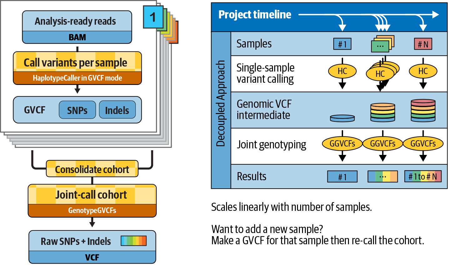
Figure 6-8. The GVCF workflow improves the scaling of joint calling and solves the N + 1 problem.

The very first step is to call variants with HaplotypeCaller per sample in reference confidence mode, also colloquially called GVCF mode, which generates an intermediate file called a GVCF. We cover the GVCF format in more detail in the hands-on exercise portion of this section; for now, just consider that it is an intermediate output that contains information for every single position of the genome territory covered by the analysis, including the many positions for which the tool did not see any evidence of variation.

After we have GVCFs for all the samples that we want to joint-call, we consolidate them into a GenomicsDB datastore, which is similar to a database that takes the form of a collection of files. We can then perform joint-calling to produce the raw cohort callset, which contains variant calls made across all samples, with detailed genotype information for each sample. This step, shown in Figure 6-9, runs quite quickly and can be rerun at any point when samples are added to the cohort, thereby solving the N + 1 problem.

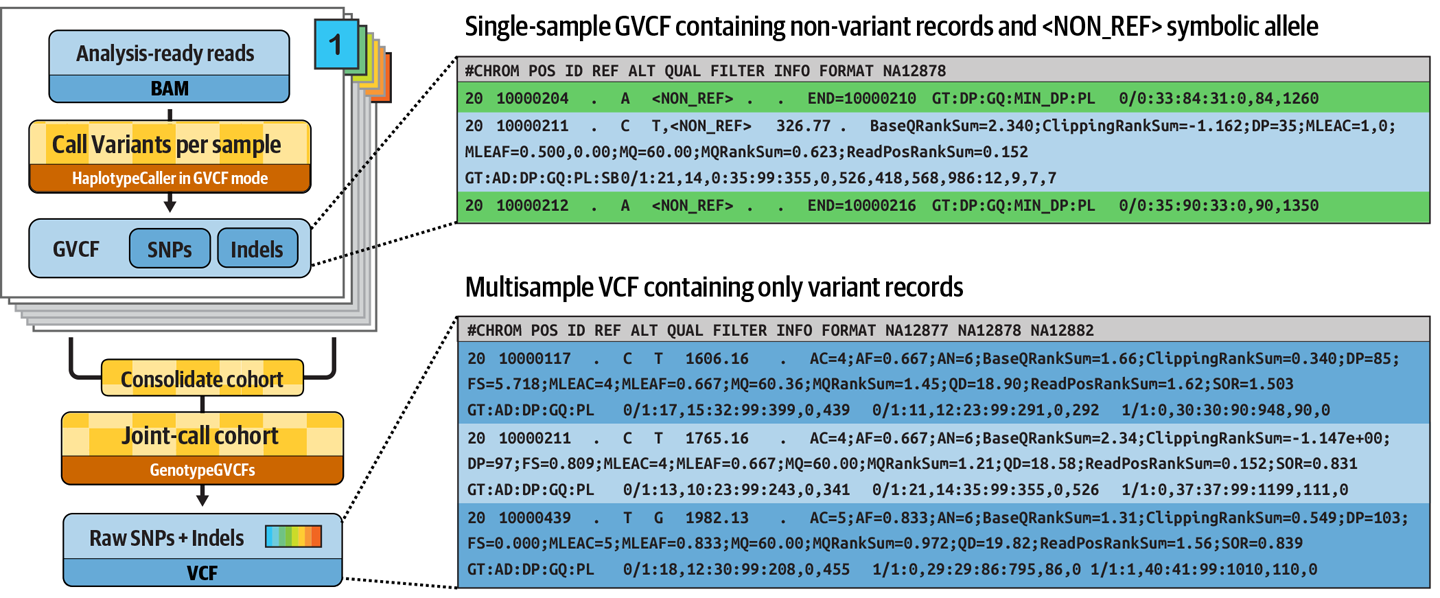
Figure 6-9. Progression from per-sample GVCFs to final cohort VCF.

This cohort-wide analysis empowers sensitive detection of variants even at difficult sites, and produces a squared-off matrix of genotypes that provides information about all sites of interest in all samples considered, which is important for many downstream analyses.

Whew, that was a lot of theory. Are you ready to get your hands back on the keyboard for a few exercises? That’s right; it’s time to start up your VM again and jump back into your GATK container, just as you did in Chapter 5. You’re going to work from within the /home/book/data/germline directory and use the same sandbox directory that you created in Chapter 5.

Calling Variants per Sample to Generate GVCFs

First, we’re going to run HaplotypeCaller in GVCF mode on the mother BAM file we played with in Chapter 5. It’s almost exactly the same command, except now we’re adding the -ERC GVCF argument and naming the output with a .g.vcf extension (plus .gz for compression purposes). Make sure you run this from within the /home/book/data/germline directory in the container on your VM:

# gatk HaplotypeCaller \
    -R ref/ref.fasta \
    -I bams/mother.bam \
    -O sandbox/mother_variants.200k.g.vcf.gz \
    -L 20:10,000,000-10,200,000 \
    -ERC GVCF

This produces a GVCF file that contains likelihoods for each possible genotype for the variant alleles, including a symbolic allele, <NON-REF> in the ALT column. This symbolic allele is present in all records, whether they are variant records or nonvariant records. You can view what the calls look like the same way as before, using the zcat tool, grep, to get rid of the header lines, and head to limit the number of lines you want to look at:

# zcat sandbox/mother_variants.200k.g.vcf.gz | grep -v '##' | head -3
#CHROM  POS     ID      REF     ALT     QUAL    FILTER  INFO    FORMAT  NA12878
20      10000000        .       T       <NON_REF>       .       .
END=10000008    GT:DP:GQ:MIN_DP:PL      0/0:16:48:16:0,48,497
20      10000009        .       A       <NON_REF>       .       .
END=10000009    GT:DP:GQ:MIN_DP:PL      0/0:16:32:16:0,32,485

These are nonvariant sites for which HaplotypeCaller found no evidence of variation. The first is a block that covers positions 20:10,000,000 to 20:10,000,008, whereas the second covers only position 20:10,000,009. If you look a little further in the file, you’ll also find some actual variant calls like this one:

20      10000117        .       C       T,<NON_REF>     283.60  .
BaseQRankSum=-0.779;DP=23;ExcessHet=3.0103;MLEAC=1,0;MLEAF=0.500,0.00;
MQRankSum=1.044;RAW_MQandDP=84100,23;ReadPosRankSum=0.154
GT:AD:DP:GQ:PL:SB       0/1:11,12,0:23:99:291,0,292,324,327,652:9,2,9,3

Now see what GVCFs look like in the IGV. We supply precomputed GVCF files for all three members of the CEU Trio (Mother, Father, and Son), but you could generate them yourself in the same way as the first from the BAMs we also provide.

Start a new session to clear your IGV screen (File > New Session) and then load the GVCF for each CEU Trio member (gvcfs/mother.g.vcf, gvcfs/father.g.vcf, gvcfs/son.g.vcf) using the paths to the file locations in the book bucket.1 This time, be sure to provide the index file paths to IGV because it is unable to get them automatically for compressed files. Zoom in on the genomic coordinates 20:10,002,371-10,002,546. You should see something like Figure 6-10.

Notice anything different in the GVCF compared to the VCFs that you saw in Chapter 5? Instead of just seeing a few variant sites, you see many gray blocks. If you click one to examine the details of the call, you’ll see that the genotype assignment is homozygous reference, and the position information includes an END coordinate, which indicates that the block covers an interval of one or more bases. These blocks represent intervals where the sample appears to be nonvariant and for which the contiguous sites it covers have similar genotype likelihoods. HaplotypeCaller groups nonvariant sites into blocks during the calling process based on their likelihoods as a way of compressing the information in the GVCF without losing useful information in areas where there is more variability in the quality of the available information.

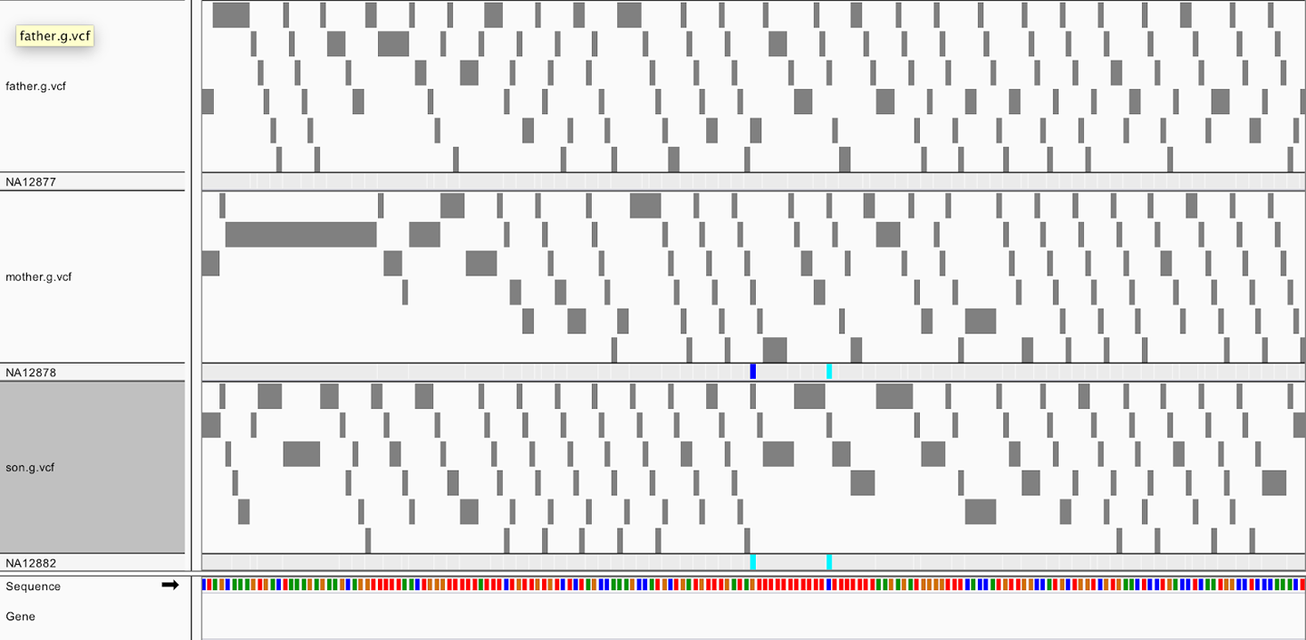
Figure 6-10. GVCFs viewed in IGV show tiled nonvariant blocks.

The HaplotypeCaller calculates the likelihoods for these GVCF blocks using an abstract nonreference allele that represents all the possible variation that it did not observe; they serve as an estimate of how confident we are that these sites are truly nonvariant. Later, the joint calling step will retain only sites that are likely enough to be variant compared to the reference in at least one sample in the cohort. For variant sites, the nonreference allele serves to estimate the likelihood that a new allele seen in one sample was missed in the other samples.

Consolidating GVCFs

For the next step, we need to consolidate the GVCFs into a GenomicsDB datastore in order to improve scalability and speed in the next step, joint genotyping. That might sound complicated, but it’s actually very straightforward. Let’s try running this on two of the samples we have available:

# gatk GenomicsDBImport \
    -V gvcfs/mother.g.vcf.gz \
    -V gvcfs/father.g.vcf.gz \
    --genomicsdb-workspace-path sandbox/trio-gdb \
    --intervals 20:10,000,000-10,200,000

This will create a new directory called trio-gdb containing the datastore contents. We named our datastore trio-gdb aspirationally, because, ultimately, we want to include all three samples from the family in the analysis, but we’re pretending that the son’s sample hasn’t been completed yet—some kind of delay happened in the lab.

The way the consolidated GVCF information is represented in the database makes it difficult to examine directly, so if we want to visualize it, we need to extract the combined data from the GenomicsDB database using SelectVariants:

# gatk SelectVariants \
    -R ref/ref.fasta \
    -V gendb://sandbox/trio-gdb \
    -O sandbox/duo_selectvariants.g.vcf.gz

This time, when you run zcat to view the contents, you’ll see that you now have two columns with genotype information, one for each of the samples that we originally included:

$ zcat sandbox/duo_selectvariants.g.vcf.gz | grep -v '##' | head -3
#CHROM  POS     ID      REF     ALT     QUAL    FILTER  INFO    FORMAT  NA12877 NA12878
20      10000000        .       T       <NON_REF>       .       .
END=10000001    GT:DP:GQ:MIN_DP:PL      ./.:15:39:15:0,39,585 ./.:16:48:16:0,48,497
20      10000002        .       G       <NON_REF>       .       .       .
GT:DP:GQ:MIN_DP:PL      ./.:15:39:15:0,39,585 ./.:16:48:16:0,48,497

This extraction step is not part of the routine pipeline, but it can be helpful for understanding what happens under the hood when we combine GVCFs from multiple samples. It also comes in handy when we need to troubleshoot unexpected or problematic results.

OK, so we just combined the GVCFs from the mother and father samples. Now, let’s imagine that the son’s sample was just delivered, and we want to add it to our datastore without having to rerun everything. We’re going to use the GenomicsDBImport tool  again, but this time we’re going to make it update the existing datastore (rather than creating a new one) by using --genomicsdb-update-workspace-path instead of --genomicsdb-workspace-path to specify the datastore:

# gatk GenomicsDBImport \
    -V gvcfs/son.g.vcf.gz \
    --genomicsdb-update-workspace-path sandbox/trio-gdb

You can check that the datastore was updated with the son’s samples by running the same basic extraction command as before:

# gatk SelectVariants \
    -R ref/ref.fasta \
    -V gendb://sandbox/trio-gdb \
    -O sandbox/trio_selectvariants.g.vcf.gz

Run zcat again to view the contents of the new file (which we named slightly differently), and you should now see three columns with genotype information:

$ zcat sandbox/trio_selectvariants.g.vcf.gz | grep -v '##' | head -3
#CHROM  POS     ID      REF     ALT     QUAL    FILTER  INFO    FORMAT  NA12877 NA12878 NA12882
20      10000000        .       T       <NON_REF>       .       .
END=10000001    GT:DP:GQ:MIN_DP:PL      ./.:15:39:15:0,39,585 ./.:16:48:16:0,48,497   
./.:20:60:20:0,60,573
20      10000002        .       G       <NON_REF>       .       .       .
GT:DP:GQ:MIN_DP:PL      ./.:15:39:15:0,39,585 ./.:16:48:16:0,48,497   ./.:20:57:20:0,57,855

Success! You just defeated the N + 1 problem by adding samples incrementally to a GenomicsDB datastore.

This ability to add samples incrementally to a GenomicsDB datastore is subject to a few limitations. The tool documentation recommends making a backup of the datastore before proceeding to update it, because any interruptions of the process could corrupt the data and leave it in an unusable state. In addition, it’s not possible to specify new intervals when updating an existing datastore; the tool will automatically use the intervals that were originally used to create it. That’s why our second GenomicsDB​Im⁠port command didn’t include any intervals.

It’s important to understand that the process of consolidating GVCFs that you just worked through is not equivalent to the joint genotyping step, which we tackle in a minute. We can’t consider variants in the resulting merged GVCF as having been called jointly. No analysis was involved; this is really just a matter of organizing the information differently for logistical reasons.

Note

Prior to GATK4, this step was done through hierarchical merges with a tool called CombineGVCFs. That tool is included in GATK4 for legacy purposes, but performance is far superior when using GenomicsDBImport, as in the previous example. 

Applying Joint Genotyping to Multiple Samples

It’s time to apply the joint calling tool, GenotypeGVCFs, to the consolidated GVCF or GenomicsDB datastore. The tool will look at the available information for each site from both variant and nonvariant samples across all the samples in the cohort and will produce a VCF containing only the sites that it found to be variant in at least one sample:

# gatk GenotypeGVCFs \
    -R ref/ref.fasta \
    -V gendb://sandbox/trio-gdb \
    -O sandbox/trio-jointcalls.vcf.gz \
    -L 20:10,000,000-10,200,000

Finally, we have our multisample callset! If we compare that final VCF to the original GVCFs, we’ve now removed sites that were nonvariant in all the samples that we joint-called, and the symbolic <NON_REF> allele is gone, as well, because it has served its purpose:

# zcat sandbox/trio-jointcalls.vcf.gz | grep -v '##' | head -3
#CHROM  POS   ID    REF   ALT   QUAL  FILTER  INFO    FORMAT  NA12877 NA12878 NA12882
20      10000117      .     C     T     1624.94 .
AC=4;AF=0.667;AN=6;BaseQRankSum=1.91;DP=85;ExcessHet=3.9794;FS=5.718;MLEAC=4;MLEAF=0.667;
MQ=60.25;MQRankSum=1.04;QD=19.12;ReadPosRankSum=2.21;SOR=1.503       
GT:AD:DP:GQ:PL    0/1:17,15:32:99:399,0,439
0/1:11,12:23:99:291,0,292       1/1:0,30:30:90:948,90,0
20      10000211      .     C     T     1783.94 .
AC=4;AF=0.667;AN=6;BaseQRankSum=2.63;DP=96;ExcessHet=3.9794;FS=0.809;MLEAC=4;MLEAF=0.667;
MQ=60.00;MQRankSum=0.00;QD=18.78;ReadPosRankSum=-4.210e-01;
SOR=0.831 GT:AD:DP:GQ:PL    0/1:13,10:23:99:243,0,341
0/1:21,14:35:99:355,0,526       1/1:0,37:37:99:1199,111,0

The calls made by GenotypeGVCFs and HaplotypeCaller run in multisample mode should mostly be equivalent, especially as cohort sizes increase. However, borderline calls can have marginal differences; for instance, low-quality variant sites, in particular for small cohorts with low coverage. Since the release of GATK 4.1, this should be less of a problem, thanks to the introduction of a new QUAL score model (available to some earlier versions via the -new-qual flag). Alternatively, it is possible to perform joint genotyping directly with HaplotypeCaller on small cohorts.

This is what the command to run HaplotypeCaller jointly on the three samples would look like:

# gatk HaplotypeCaller \
    -R ref/ref.fasta \
    -I bams/mother.bam \
    -I bams/father.bam \
    -I bams/son.bam \
    -O sandbox/trio_jointcalls_hc.vcf.gz \
    -L 20:10,000,000-10,200,000 

You can run it if you want to compare the calls to the joint-called results we generated earlier.

Now let’s circle back to the locus we examined at the start. Load sandbox/trioGGVCF.vcf into IGV and navigate to the genomic coordinates 20:10,002,376-10,002,550. As shown in Figure 6-11, you should see the variant call on the top track and the genotypes for each of the three samples below.

Figure 6-11. Variant call with genotype assignment for the three samples.

Now we have genotypes at this site for both the father (NA12877) and son (NA12882) in addition to the mother. If you click each one, you’ll see both the mother and the son were called homozygous variant, yet the father was called homozygous reference; that is, nonvariant. Given the familial relationship for the three samples, what do you think about this set of genotype calls?

If you’re thinking it doesn’t make sense, you’re right! The evidence we have for both the mother and the child being truly homozygous variant is fairly strong, but then the father is extremely unlikely to be homozygous reference because that’s a flagrant Mendelian violation (i.e., it breaks Mendel’s rules of genetic inheritance). That would mean the son received one variant allele from his mother and one reference allele from his father, and then experienced an early mutation that produced a matching de novo variant—not impossible, but very unlikely. So two possibilities exist here; either the daddy is not the daddy (it happens more often than you want to know), or the tool made an error in one or more of the genotypes. We happen to know from other sources that NA12877’s paternity is not in question, so we need to accept that the tool made a mistake. This is not so unusual when there is some ambiguity in the data, especially when homopolymers are involved, as is the case here.

In fact, we ran a few tests with other pipelines and found that other variant callers also stumbled on the genotype assignments for this variant in the same data. Some of them also called the father homozygous reference, whereas others called it heterozygous. So this is a site in the genome where joint calling allows us to make a good variant call, in that we are confident that one or more samples in the group show some variation there, but some of the individual genotypes might be questionable. How do we deal with this? Well, we’re going to put this problem in the fridge for now, because our first order of business after calling is filtering out the bad variant calls, which does not involve taking individual genotypes into account. However, when that’s done, we’ll circle back to deal with the genotypes using a process called Genotype Refinement.

Filtering the Joint Callset with Variant Quality Score Recalibration

At this point in the variant discovery process, we have in hand a set of raw variant calls, but we know that some of our raw calls are most probably artifacts, given that the caller is explicitly designed to be very permissive. That is why we now need to filter the variant calls to distinguish those that are most likely to be real variants in the biological material from those that are most probably just artifacts introduced by biochemical processes or technical errors.

In Chapter 5, we practiced hard filtering, an approach to filtering variants that involves setting thresholds for individual variant context annotations. That approach can produce reasonable results in the hands of an experienced analyst, but it is labor intensive and difficult to extend consistently across different studies and datasets. For a more scalable and standardizable solution, we look to machine learning approaches that enable us to build models of what real variants and artifacts look like in our data, respectively.

Machine Learning in the GATK

Machine learning is a subfield of data science related to statistics. GATK analytical tools all use some kind of statistical technique; in some cases, the key algorithms belong to the machine learning family. Classic GATK machine learning methods that have been around since the early days of GATK include the aforementioned BQSR and Variant Quality Score Recalibration. In Variant Quality Score Recalibration (VQSR), the core algorithm is a Gaussian mixture model that aims to classify variants based on how their annotation values cluster, given a training set of high-confidence variants.

Meanwhile, an increasingly popular subfield of machine learning called deep learning uses techniques based on neural networks, a type of algorithm that mimics neural pathways in animal brains. Deep learning has been around for a long time, but until recently, neural networks were too computationally intensive to tackle anything more than contrived problems. Now, thanks to recent technological developments, they can tackle much bigger problems, and have become intensely popular as a way to pursue artificial intelligence. Later in this chapter, you’ll have the opportunity to try out GATK tools that apply neural networks to classify and filter variants in a single sample.

That being said, new advances in machine learning approaches in genomics are not limited to deep learning. The GATK Best Practices pipeline for germline copy-number variant (gCNV) discovery uses a type of machine learning algorithm called a Probabilistic Graphical Model (PGM) to deliver gCNV calling on either a single sample or a cohort of samples. It outperforms established methods in the field significantly, both in terms of accuracy and of computational scalability. Unfortunately we don’t cover it in this book, but you can learn more about it in the relevant GATK documentation.

When filtering a multisample callset, the GATK Best Practices recommendation is to use the Variant Quality Score Recalibration (VQSR) method. This method involves using variant context annotations from variants that are present in a training set to model how variants that are likely to be real cluster together. Then, it’s a matter of applying the model to all of the variants in our callset of interest. You can think of this as a process in which we’re measuring where each variant lies relative to the clusters of real variants across all of the annotation dimensions. The closer a variant is to a cluster, the more likely it is to be real. Of course, this can be difficult to visualize when we take all the annotations into account because there are more than the three that our puny human brains are generally limited to handling at a time. So we usually represent subsets of the model by making pairwise scatter plots of two annotations at a time to visualize the clustering process, as shown in Figure 6-12.

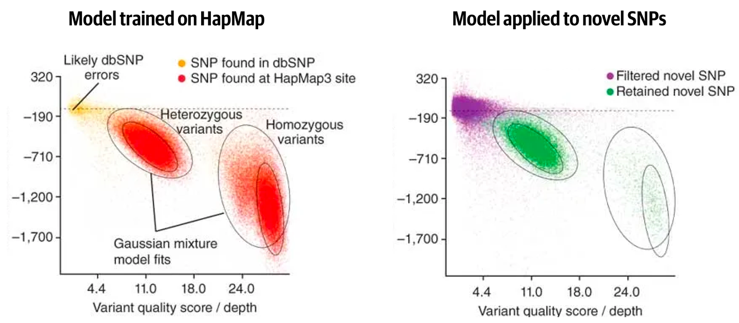
Figure 6-12. Gaussian clusters learned from a training set are applied to novel variant calls.

In practice, the VQSR tools use the model to assign a new confidence score to each variant, called VQSLOD, which is more reliable than the QUAL confidence score originally calculated by the caller because it takes more information into account. Specifically, this new score takes into account all the variant context annotations that would be informative enough for hard filtering, and the resulting score encapsulates the information contributed by every one of those annotations in a single value.

In Figure 6-13, each dot at the bottom is an individual variant, plotted where its annotation value falls on the x-axis. The variants clustering to the left are considered good based on preliminary scoring, whereas those on the right are considered bad. The density curves above them show the positive model (left) and negative model (right), respectively, representing the proportion of variants with corresponding annotation values. The VQSLOD for a given variant is the log ratio of the variant’s probabilities of belonging to the positive model and to the negative model, respectively. Here we’re showing how this applies to a single annotation; in reality, we’ll calculate the VQSLOD score based on multiple annotations, so the tools will do some additional mathematical integration that we don’t show here to produce a single unified score.

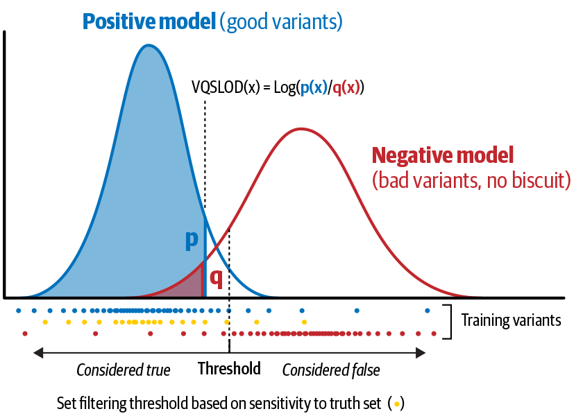
Figure 6-13. How the VQSLOD score is calculated for an individual annotation.

This single unified score is very convenient because it means that all that remains for us to do is to set a filtering threshold for that single score instead of trying to set thresholds for all the annotations separately. Contrast that to what we covered on the topic of hard filtering; you can see this is much handier.

So how do we set a threshold on that one score? Indirectly. There is no absolute scale that tells us what is a good VQSLOD. Instead, given a truth set that overlaps substantially with our callset, we can use a truth sensitivity threshold as a more meaningful proxy for finding the “right” VQSLOD score. This means that we can specify a target sensitivity—for example, 99.9%—and have the tools internally determine whatever VQSLOD would be appropriate for the filtering process to guarantee that 99.9% of the variants we know are true will still be considered real in the resulting filtered callset. In other words, this comes down to saying, “Filter my callset with whatever VQSLOD would give me back 99.9% of the variants that I know are true in this callset.” That target sensitivity value itself is not an absolute recommendation, given that different projects might require different levels of sensitivity and precision, but at least it provides a principled basis for the analyst to choose their threshold.

We don’t provide hands-on exercises for this step, because the VQSR algorithm is greedy for data—it needs to see all the variant data at once—so it’s difficult to create an example case that will run in a short amount of time. Instead, here are example commands for the two steps involved in VQSR.

To build the model and apply it to a joint-called dataset and calculate VQSLOD scores for the variants it contains, we would use VariantRecalibrator, as follows:

gatk VariantRecalibrator \
   -R reference.fasta \
   -V jointcalls_hc.vcf.gz \
   --resource:hapmap,known=false,training=true,truth=true,prior=15.0 \
   hapmap_sites.vcf.gz \
   --resource:omni,known=false,training=true,truth=false,prior=12.0 \
   1000G_omni2.5.sites.vcf.gz \
   --resource:1000G,known=false,training=true,truth=false,prior=10.0 \
   1000G_phase1.snps.high_conf.vcf.gz \
   --resource:dbsnp,known=true,training=false,truth=false,prior=2.0 dbsnp.vcf.gz \
   -an QD -an MQ -an MQRankSum -an ReadPosRankSum -an FS -an SOR \
   -mode SNP \
   -O output.recal \
   --tranches-file output.tranches

This is one of the longer GATK commands you’re likely to encounter, so it’s worth taking a minute to go over what it involves. In addition to the reference genome of the VCF of joint calls, which are its main input, the command takes in a set of resource files (via the --resource parameter) that play an essential role in the modeling process. These should be sets of variant calls that have been previously reported and curated to some degree of confidence expressed by the prior metric. Here, we show the resources that are used for human genome analysis; for other organisms, you would have to adapt the resources you use accordingly. The -an parameters specify the variant context annotations that we want to use in the recalibration process, and here we show the default recommendations provided by the GATK team. The -mode parameter controls which kind of variants the tool should recalibrate. Because of some key differences between how SNPs and indels show up in the sequence, we need to recalibrate them in separate passes, so we would run this once in SNP mode and then once again in INDEL mode. Finally, the command will produce two output files: the main recalibration file (output.recal), and a tranches file (output.tranches) that maps several confidence levels to specific VQSLOD cutoffs.

After we’ve run that, we still need to choose a confidence level to use as sensitivity threshold and actually generate a filtered VCF for our callset, which we would do by using ApplyVQSR, as follows:

gatk ApplyVQSR \
   -R reference.fasta \
   -V jointcalls_hc.vcf.gz \
   -O jointcalls_filtered.vcf.gz \
   --truth-sensitivity-filter-level 99.9 \
   --tranches-file output.tranches \
   --recal-file output.recal \
   -mode SNP

In this command, we’re mostly just feeding in the reference, original data and the two files output by VariantRecalibrator, the tranches files, and the recalibration file. We also pass in the confidence level we want to use with the --truth-sensitivity-filter-level argument, using 99.9% because it is the recommended default for SNPs in human genomic analysis, but keep in mind that this is something you would need to decide based on your experimental goals. The final output of the procedure will be the filtered callset, which will still contain all the original variant sites, but the ones that fail to pass the VQSLOD threshold will be marked as filtered and ignored in downstream analyses.

The downside of how variant recalibration works is that the algorithm requires high-quality sets of known variants to use as training and truth resources, which for many organisms are not yet available. It also requires quite a lot of data in order to learn the profiles of good versus bad variants, so it can be difficult or even impossible to use on small datasets containing only one or a few samples, on targeted sequencing data, on RNAseq, and on nonmodel organisms. If for any of these reasons you cannot perform variant recalibration on your data, you will need to use either the neural networks–based technique referenced in “Single-Sample Calling with CNN Filtering”, or hard filtering, which consists of setting flat thresholds for specific annotations and applying them to all variants equally, as described in Chapter 5.

You can learn more about the variant recalibration algorithm from its documentation and see these tools in action in the reference implementation of the joint genotyping workflow.

Refining Genotype Assignments and Adjusting Genotype Confidence

Now that we have filtered our callset at the site level, we can be reasonably confident that we have the right variant calls, but as we observed earlier, some unresolved ambiguity might remain at the genotype level. For studies that require high-quality genotype information (sooo...most of them) we’re going to add on an optional step called Genotype Refinement that uses supplemental sources of information like pedigree (i.e., familial relationships) and allele frequencies observed in relevant populations to refine genotype assignments. Where applicable, this will lead us to adjust our confidence in specific genotypes or even change what genotype we assign.

Let’s apply this to the two “problem” calls we produced for the mother-father-son trio earlier—and yes, we’re back to working hands-on in the GATK container on your VM. In the command that follows, we provide the genotype refinement tool, CalculateGenotypePosteriors, with a pedigree file that describes how the three individuals are related (mother, father, and child) and a sites-only VCF file that contains allele frequencies observed in a large database of known variation called gnomAD:

# gatk CalculateGenotypePosteriors \
    -V sandbox/trio-jointcalls.vcf.gz \
    -ped resources/trio-pedigree.ped \
    --supporting-callsets resources/af-only-gnomad.vcf.gz \
    -O sandbox/trio-refined.vcf.gz

Run that and then load the resulting VCF into IGV and check out the genotype assignment we now have for the father. Zoom in on the genomic coordinates 20:10,002,438-10,002,479. What happened here? Between the trio pedigree and the population file, the tool decided that the father’s genotype was highly questionable, so it downgraded the genotype quality score, as depicted in Figure 6-14, to the point that this genotype would be filtered out as being unreliable for downstream analysis.

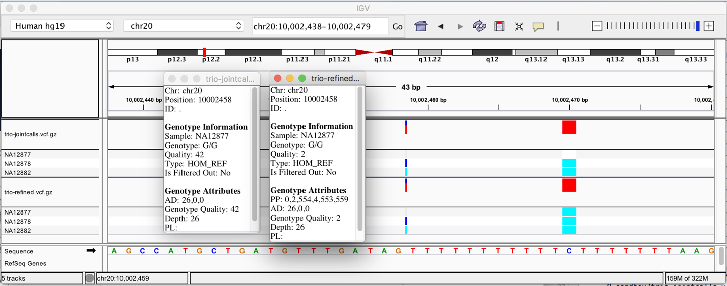
Figure 6-14. Genotype assignments corrected on the basis of pedigree and population priors.

It’s important to understand that the tool does not “brute-force” the genotype assignment; if we had a confident genotype call to begin with, the external information would not be sufficient to overturn the caller’s initial judgment. However, when we have a low-confidence call, where the caller is essentially telling us “here’s my best guess but I’m probably wrong,” the supplemental information allows us to resolve the ambiguity and rescue a variant call that might otherwise be unusable for downstream analysis, as in the case of the SNP. Or, as in the case of the indel, it recalibrates the confidence we have in the genotype call.

Next Steps and Further Reading

This concludes the whistle-stop tour of the joint discovery workflow, at least as far as this book is concerned. There is a lot more to learn about how the algorithms and tools that we presented here operate, and about how you can customize these commands to suit your particular data and experimental goals. We recommend that you check out the relevant documentation on the GATK website as well as the reference implementations of the workflows, though you might benefit from waiting until you’ve worked through the rest of this book to tackle those. If you’re not familiar with WDL workflows, you’ll especially want to read Chapter 8 through Chapter 11 first, in which we teach you what you need to know to decipher the workflows and use them effectively for your own work.

Before we move on to somatic variant calling, however, let’s consider the case of single-sample calling, which is a bit of a niche use case compared to joint calling but is of great importance in clinical genomics.

Single-Sample Calling with CNN Filtering

As discussed earlier, sometimes we are constrained to analyzing a single sample at a time. When that’s the case, we don’t need to follow the GVCF workflow; instead, we can simply apply the basic command for HaplotypeCaller, as shown in the very first exercise in this chapter. However, that leads us to having too little data (specifically, too few variants) for filtering with VQSR, which, as we have noted, is a very greedy algorithm that requires lots of data.

Over the years, the GATK development team tried a variety of algorithms to address this issue. Then, a breakthrough: the advent of “cheap and easy” machine learning tools, and the rise of deep learning in particular, empowered the team to apply a technique called Convolutional Neural Networks, or CNN. This new approach proved to be impressively effective for single-sample germline short variant calling, performing well even on indels, which are traditionally the more difficult problem in this space compared to SNVs.

CNNs Applied to Variant Calling

If you’re not familiar with CNNs, you’re not alone—and the good news is, you don’t really need to understand every detail of the theory to use them, just like you don’t need to master the intricacies of internal combustion engines in order to drive a car. But it can be helpful to get a sense of what’s under the hood, so let’s go over the main points together.

First, what’s with the name? The neural networks part refers to a type of machine learning techniques that are loosely modeled after neural connections in the human brain and specialize in recognizing patterns in numerical data. The convolution bit in the CNN name refers to the specific type of mathematical operation used to process data. From the Latin convolvere, meaning roll together, convolution involves combining signals from different sources of information or from different scales. In the case of the GATK CNN algorithm, this allows the tool to capture features like 10 basepair sequence motifs.

A commonly described application of neural networks is for classifying images. The internet has many examples, and, of course, it’s the internet, so the most popular ones compare various kinds of dogs to items that are most decidedly not dogs. This leads to classic memes like “sheepdog or mop,” “chihuahua or muffin,” “puppy or bagel,” and, our personal favorite, “labradoodle or fried chicken,” as shown in Figure 6-15, taken from an NPR article. It turns out that although it’s fairly trivial for a minimally focused human brain to make these distinctions on sight, describing the relevant rules to a computer is quite a bit more challenging.

Figure 6-15. Labradoodle or fried chicken? (Source: Karen Zack, @teenybiscuit)

Doing so involves detecting edges in the picture to identify the minimal silhouette, divested of any unhelpful visual noise, that will allow us to make the distinction we’re after. In image analysis, this is done separately for the red, green, and blue channels that images are composed of. The resulting edge maps are then combined into a tensor, a data structure that provides a way to stack information from different sources. Then, the tensors representing various images are fed into the neural network and grouped together based on similarities. Long story short, if we provide a training set with images that are labeled one way or another, the algorithm will be able to cross-reference how the labeled images were grouped with the rest and therefore produce labels for all images.

So how does this relate to variant calls? The basic idea is that we have different types of information available about our variant calls: variant context annotation values, reference sequence context, and optionally read data, that we want to use to make a judgment about the veracity of each call. We encode all that information into tensors just like the edge maps in the image analysis case, and feed the tensors to a modeling architecture that can detect predictive features in the bundle of information provided.

This is a deep topic about which there is a lot to learn, but it can be quite…convoluted, so to speak. In the interest of not turning this book into a treatise on machine learning, let’s skip straight to how it differs from previous approaches and how we apply the relevant tools in practice.

Overview of the CNN Single-Sample Workflow

At a very high level, the procedure for applying CNN to variant calling appears similar to VQSR, which we covered earlier: the tools build a model of what real variation looks like based on training sets, and when we apply that model to our callset, we get a new confidence score for each of our variants. Under the hood, however, the modeling architecture is wildly different—and quite a bit more complicated. Again, the good news is that you don’t need to care too much about how it works at that level, as long as you understand its key benefit: we can include more information than just the variant context annotations in the modeling process. So far, we were limited to using annotations, which are essentially summaries of the original sequence data, for both hard filtering and VQSR.

Now, with CNN, we can also take advantage of what we know about the reference sequence context, and we can even take into account the raw read data itself. That gives us more power to discriminate between real variants and artifacts, especially for indels in difficult areas of the genome where the sequence context is littered with short tandem repeats (repetitions of the same few bases, like TATATATATA) and homopolymers (runs of the same one base, like AAAAAAAAAA) that are classic confounding factors for variant calling. In practice, we’ll refer to the basic approach that uses annotations supplemented with just reference context information as 1-D CNN, and the somewhat more sophisticated approach that also uses read data as 2-D CNN.

Another important benefit of how the CNN modeling works is that it allows us to create models that can be applied out of the box to new datasets as long as they are similar enough to the original training data in terms of experimental design and technology (i.e., how the sequencing was done). This is also a big difference compared to the VQSR method, which requires that you train a new model for every new callset that you want to filter. The GATK package includes a set of precomputed models trained on highly validated callsets produced from reference datasets such as SynDip, GiaB, and Platinum Genomes. For convenience, the GATK CNN tools are set to use the appropriate default model (1D or 2D modeling) based on which inputs are provided (or not). That being said, you can train your own models if you prefer.

Let’s run through the main two options for running with a precomputed model. You’ll see that this method is easy to use even if you don’t understand the underlying algorithm in detail. Note that because the CNN tools are very new as of this writing, the examples use a separate set of resource files, so you now need to change our working directory within the GATK container: you were previously in /home/book/data/germline, so now you need to change your working directory to /home/book/data/cnn. To be clear, the CNN tools are intended for germline variant discovery; the naming and file bundle structure simply reflects the fact that these tools have a somewhat special status for now:

# cd ../cnn
# mkdir sandbox
# ls 
bams  ref  resources  sandbox  vcfs

As previously, you create a sandbox for collecting the outputs of the commands that you’re going to run.

Applying 1D CNN to Filter a Single-Sample WGS Callset

The simplest form, or architecture, of CNN modeling available in GATK is called 1D for one-dimensional. That term may seem a little misleading because it takes into account variant context annotations and reference sequence context, all of which most of us would probably not think of as representing a single dimension. Nevertheless, as with much of the machine learning jargon, it might be best to just accept it and move on with your life. If it helps, you can think of the dimensions as if you were visualizing the read data in IGV. 1D is a line, which is the reference. 2D is that reference line and also the depth of all the reads.

Conveniently, the GATK package includes a precomputed 1D model that is compatible with our tutorial data. To apply it to our callset of interest, we simply feed our VCF to the CNNScoreVariants tool, which will calculate a new confidence score called CNN_1D for each variant. The precomputed model is used by default unless we explicitly specify a model file on the command line (we demonstrate that usage later in this section):

# gatk CNNScoreVariants \
    -R ref/Homo_sapiens_assembly19.fasta \
    -V vcfs/g94982_b37_chr20_1m_15871.vcf.gz \
    -O sandbox/my_1d_cnn_scored.vcf

This produces a new VCF file in which our variants have not yet been filtered, just annotated with the new score as well as sensitivity tranche information. To actually apply a filtering rule, we use the same sensitivity-based logic as VQSR, providing known variant callsets as resources and the desired thresholds to the generalized filtering tool FilterVariantTranches:

# gatk FilterVariantTranches \
    -V sandbox/my_1d_cnn_scored.vcf \
    -O sandbox/my_1d_cnn_filtered.vcf \
    --resource resources/1000G_omni2.5.b37.vcf.gz \
    --resource resources/hapmap_3.3.b37.vcf.gz \
    --info-key CNN_1D \
    --snp-tranche 99.9 \
    --indel-tranche 95.0 

We choose 99.9% and 95.0% for the SNP and indel sensitivity thresholds because those are the same recommended defaults as we encountered in the VQSR filtering section, but remember that the same admonition applies: you should choose these settings based on your experimental goals.

The tool helpfully includes a filtering summary at the end of its run:

13:47:51.613 INFO  ProgressMeter - Traversal complete. Processed 31742 total
variants in 0.0 minutes.
13:47:51.614 INFO  FilterVariantTranches - Filtered 303 SNPs out of 12929 and
filtered 669 indels out of 2932 with INFO score: CNN_1D.

This command produces the filtered VCF in which variants are annotated with the modeling verdict in the FILTER field: PASS for variants classified as real and the name of the tranche for variants classified as artifacts. The tool accepts an optional --invalidate-previous-filters flag (not used here) that allows us to clear any previously annotated filtering information if desired. This is what the output looks like for the preceding command:

# cat sandbox/my_1d_cnn_filtered.vcf | grep -v '##' | head -3
#CHROM  POS     ID      REF     ALT     QUAL    FILTER  INFO    FORMAT  NA12878
20      1000072 rs6056638       A       G       998.77  PASS
AC=2;AF=1.00;AN=2;CNN_1D=3.256;DB;DP=32;ExcessHet=3.0103;FS=0.000;MLEAC=2;MLEAF
=1.00;MQ=60.00;POSITIVE_TRAIN_SITE;QD=31.21;SOR=0.818;VQSLOD=20.79;culprit=MQ
GT:AD:DP:GQ:PL  1/1:0,32:32:96:1027,96,0
20      1000152 rs6056639       C       T       678.77  PASS
AC=2;AF=1.00;AN=2;CNN_1D=2.313;DB;DP=28;ExcessHet=3.0103;FS=0.000;MLEAC=2;MLEAF
=1.00;MQ=60.00;POSITIVE_TRAIN_SITE;QD=24.24;SOR=0.693;VQSLOD=18.18;culprit=QD
GT:AD:DP:GQ:PL  1/1:0,28:28:81:707,81,0

If you look at more lines of output, you can find sites like this candidate indel call that has been filtered out by the 1D CNN modeling:

20      1012919 rs34579666      CT      C       439.73
CNN_1D_INDEL_Tranche_95.00_100.00       AC=2;AF=1.00;AN=2;CNN_1D=-2.925;DB;DP=31;
ExcessHet=3.0103;FS=0.000;MLEAC=2;MLEAF=1.00;MQ=59.62;POSITIVE_TRAIN_SITE;
QD=19.12;SOR=1.708;VQSLOD=3.87;culprit=SOR  GT:AD:DP:GQ:PL1/1:0,23:23:67:477,67,0

Note

You might have noticed that, unlike for the VQSR protocol, we did not need to run the CNN model application and filtering on SNPs and indels separately. Algorithmically, these tools still treat the two variant classes differently, just like the VQSR tools, but they handle this internally for us. This is a deliberate decision on the part of the developers to make the tools easier to use.

Applying 2D CNN to Include Read Data in the Modeling

As noted earlier, the CNN tools are capable of taking in the read data underlying the variant calls that we want to filter. This might seem redundant with the variant context annotations, which are, after all, intended to summarize the salient aspects of the read data in a more compact form. Yet that is one of their main flaws, given that the act of summarizing the information causes us to lose some of the more fine-grained detail in the reads.

That puts us at the mercy of two limiting factors: the fidelity of the mathematical formula chosen to summarize the data, and the imagination of the developers who decided which aspects of the data would be useful for filtering purposes. Even though it is arguably not difficult to identify a few heuristics that are bound to play a big role in predicting variant quality for the majority of calls—some form of coverage evaluation, strand orientation bias, and base quality, perhaps—it is much more challenging to identify the subtle effects that will tip the scales in difficult cases. That is a big part of what makes deep learning so appealing for variant filtering; it promises to identify (and quantify!) those effects for us without a ton of up-front analysis.

To include read data in the scoring process (while still using a precomputed model), we provide the CNNScoreVariants tool with a bamout produced by HaplotypeCaller, and we add the --tensor-type read_tensor argument to switch on the 2D model architecture. This will automatically activate the default precomputed 2D model, unless you specify your own on the command line:

# gatk CNNScoreVariants \
    -R ref/Homo_sapiens_assembly19.fasta \
    -I bams/g94982_chr20_1m_10m_bamout.bam \
    -V vcfs/g94982_b37_chr20_1m_895.vcf \
    -O sandbox/my_2d_cnn_scored.vcf \
    --tensor-type read_tensor \
    --transfer-batch-size 8 \
    --inference-batch-size 8

Notice that we feed a bamout file (created by HaplotypeCaller) to CNNScoreVariants when we run it the 2D mode, not just the original read data. We do this because the read alignments must match what HaplotypeCaller saw when it made the variant calls. This does mean that you need to add the -bamout argument to your initial HaplotypeCaller command when you do the variant calling step, which we don’t normally do, so it’s something you should plan for ahead of time.

Note

If you’re using a different variant caller than HaplotypeCaller that doesn’t generate a bamout equivalent, this doesn’t apply, and you simply provide the original read data. Keep in mind that if you use another local alignment caller like Platypus, you could run into the problem of calls that don’t quite match the original read mapping.

When you run the command, it produces a VCF with a new confidence score called CNN_2D annotated to each variant along with tranche information. To apply filtering, we run the FilterVariantTranches as before, switching the filtering info-key appropriately:

# gatk FilterVariantTranches \
    -V sandbox/my_2d_cnn_scored.vcf \
    -O sandbox/my_2d_cnn_filtered.vcf \
    --resource resources/1000G_omni2.5.b37.vcf.gz \
    --resource resources/hapmap_3.3.b37.vcf.gz \
    --info-key CNN_2D \
    --snp-tranche 99.9 \
    --indel-tranche 95.0 

The output is similar but not identical to what we produced using the 1D model architecture:

# cat sandbox/my_2d_cnn_filtered.vcf | grep -v '##' | head -3
#CHROM  POS     ID      REF     ALT     QUAL    FILTER  INFO    FORMAT  NA12878
20      1000072 rs6056638       A       G       998.77  PASS
AC=2;AF=1.00;AN=2;CNN_2D=7.687;DB;DP=32;ExcessHet=3.0103;FS=0.000;MLEAC=2;MLEAF
=1.00;MQ=60.00;POSITIVE_TRAIN_SITE;QD=31.21;SOR=0.818;VQSLOD=20.79;culprit=MQ
GT:AD:DP:GQ:PL  1/1:0,32:32:96:1027,96,0
20      1000152 rs6056639       C       T       678.77  PASS
AC=2;AF=1.00;AN=2;CNN_2D=5.349;DB;DP=28;ExcessHet=3.0103;FS=0.000;MLEAC=2;MLEAF
=1.00;MQ=60.00;POSITIVE_TRAIN_SITE;QD=24.24;SOR=0.693;VQSLOD=18.18;culprit=QD
GT:AD:DP:GQ:PL  1/1:0,28:28:81:707,81,0

And a little farther down, that indel we looked at earlier is still filtered out:

20      1012919 rs34579666      CT      C       439.73
CNN_2D_INDEL_Tranche_95.00_100.00
AC=2;AF=1.00;AN=2;CNN_2D=5.576;DB;DP=31;ExcessHet=3.0103;FS=0.000;MLEAC=2;
MLEAF=1.00;MQ=59.62;POSITIVE_TRAIN_SITE;QD=19.12;SOR=1.708;VQSLOD=3.87;
culprit=SOR 
GT:AD:DP:GQ:PL1/1:0,23:23:67:477,67,0

If you’d like to inspect these in more detail to compare calls filtered by one but not the other, an easy way is to load the VCFs in IGV as described previously and scroll until you find a difference like the one shown in Figure 6-16. Note the lighter colors for one of the variant call markers in the 2D_CNN track; that indicates the call was filtered.

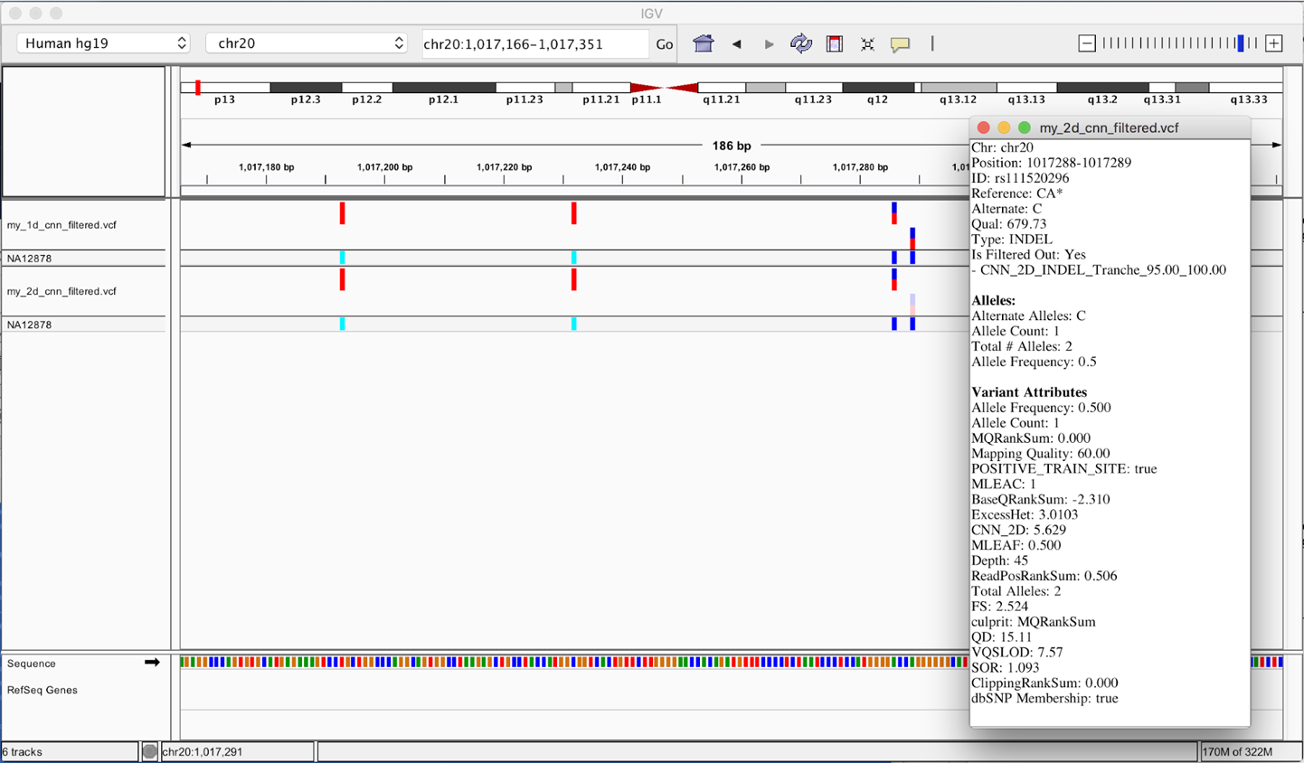
Figure 6-16. Different calls made by 1D and 2D CNN models.

Finally, keep in mind that the model provided by default is tailored to Illumina short read sequencing data from humans. It should be widely applicable also to other organisms sequenced with the same or similar technology, but the further out you go, the less fidelity you’ll get because the precomputed model will not be as good a fit for the reality of your data. At some point, you might be better off generating your own custom model. There is a Python script for training custom models that is available in the GATK repository on GitHub, but the GATK team has not yet developed formal recommendations for how to use it because it is an area of ongoing development. For additional resources, see the Best Practices documentation.

Note

This concludes the exercises for this chapter, so unless you’re moving on to the next chapter right away (what stamina!), remember to stop your VM so you don’t end up paying while you’re not playing.

Wrap-Up and Next Steps

You have now successfully worked through the most widely used germline joint variant discovery pipeline and its alternate single-sample form. You have a solid understanding of the overall logic of the pipeline, you’ve applied most of the key steps to real data, and you’ve observed the results for yourself. Next up, we tackle somatic variant discovery, mainly as it applies to cancer research.

First, we go over a few important challenges that affect the design of analytical approaches in cancer genomics. Then, we dive into the pipeline for somatic short variant analysis and work through some exercises to get a firm grasp of the key steps. After that, we branch out into the exploration of somatic copy-number alterations, which involves a very different approach compared to short variant analysis. 

1 The full file paths are gs://genomics-in-the-cloud/v1/data/germline/gvcfs/mother.g.vcf.gz, gs://genomics-in-the-cloud/v1/data/germline/gvcfs/mother.g.vcf.gz.tbi, gs://genomics-in-the-cloud/v1/data/germline/gvcfs/father.g.vcf.gz, gs://genomics-in-the-cloud/v1/data/germline/gvcfs/father.g.vcf.gz.tbi, gs://genomics-in-the-cloud/v1/data/germline/gvcfs/son.g.vcf.gz, and gs://genomics-in-the-cloud/v1/data/germline/gvcfs/son.g.vcf.gz.tbi.