Chapter 11. Running Many Workflows Conveniently in Terra
In Chapter 10, we gave you a tantalizing first taste of the power of the Cromwell plus Pipelines API combination. You learned how to dispatch individual workflows to PAPI, both directly through Cromwell and indirectly through the WDL Runner wrapper. Both approaches enabled you to rapidly marshal arbitrary amounts of cloud compute resources without needing to administer them directly, which is probably the most important lesson you can take from this book. However, as we’ve discussed, both approaches suffer from limitations that would prevent you from achieving the truly great scalability that the cloud has to offer.
In this chapter, we show you how to use a fully featured Cromwell server within Terra, a cloud-based platform operated by the Broad Institute. We begin by introducing you to the platform and walking you through the basics of running workflows in Terra. Along the way, you’ll have the opportunity to experiment with the call caching feature that allows the Cromwell server to resume failed or interrupted workflows from the point of failure. With that experience in hand, you’ll graduate to finally running a full-scale GATK Best Practices pipeline on a whole genome dataset.
Getting Started with Terra
You are just a few short hops away from experiencing the delights of a fully loaded Cromwell server thanks to Terra, a scalable platform for biomedical research operated by the Broad Institute in collaboration with Verily. Terra is designed to provide researchers with a user-friendly yet flexible environment for doing secure and scalable analysis in GCP. Under the hood, Terra includes a persistent Cromwell server configured to dispatch workflows to PAPI and equipped with a dedicated call caching database. On the surface, it provides a point-and-click interface for running and monitoring workflows as well as API access for those who prefer to interact with the system programmatically. Terra also provides rich functionality for accessing and managing data, performing interactive analysis through Jupyter Notebook, and collaborating securely through robust permissions controls. Figure 11-1 summarizes Terra’s current primary capabilities.
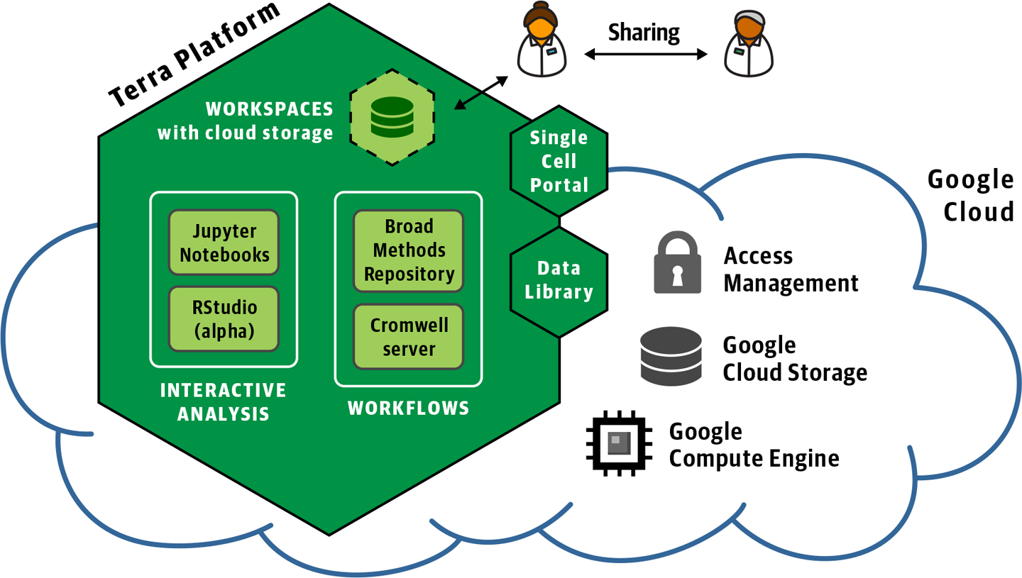
Figure 11-1. Overview of the Terra platform.
In this section, we focus on the workflow configuration, execution, and monitoring functionality through the web interface, but later in the chapter, we also dig into some interactive analysis in Jupyter.
Note
As of this writing, the Terra platform is under active development, so you likely will encounter differences between the screenshots here and the live web interface, as well as new features and behaviors. We’ll provide updated instructions and guidance regarding any major changes in the blog for this book.
Creating an Account
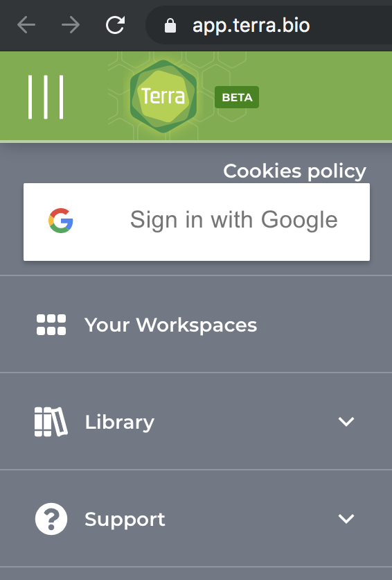
You can register for a Terra account for free. In the upper-left corner of your browser window, click the three-line symbol to expand the side menu and bring up the Sign in with Google button, as shown in Figure 11-2.
Note
Menu symbols and navigation patterns in Terra are often similar to those in the GCP console. Whenever you see the same symbols, you can safely assume they have the same purpose.
Sign in with the same account that you have been using so far—the one you used to set up your GCP account, and submit the registration form shown in Figure 11-3. The contact email can be different from the email you used to sign in; for example, if you are using a personal account to do the work but prefer to get email notifications sent to your work account. Email notifications you might receive from Terra mainly consist of notices about new feature releases and service status (such as planned maintenance or incident alerts). They are relatively infrequent, and you can opt out if you do not want to receive these notifications. The contact email you specify here is also used by the Terra helpdesk ticketing system, which will email you if you ask a question, report a bug, or suggest a feature.
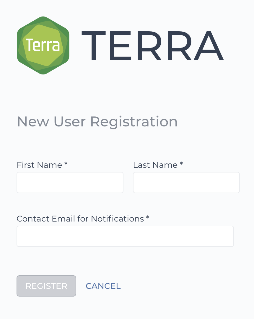
Figure 11-3. The New User Registration form.
You’ll need to accept the Terra Terms of Service. We strongly suggest that you follow the recommendation to secure your Google-linked account with two-factor authentication. Keep in mind that Terra is designed primarily to enable analysis of human patient data and includes repositories that host data funded by US government agencies with access restrictions, so security is a serious matter on the platform.
Creating a Billing Project
After you have completed the registration process, you should find yourself on the Terra portal landing page. At the top of the page, you might see a banner advertising free credits, as shown in Figure 11-4. As of this writing, you can get $300 worth of free credits to try out the platform (on top of the credits you might already be getting directly from GCP), as described in the Terra user guide. Terra is built on top of GCP, and when you do work in Terra that incurs costs, GCP directly bills your account. The Broad Institute will not charge you any surcharges for the use of the platform.
We recommend that you take advantage of the free credits opportunity, not only for the credits themselves, but also because the system will automatically set up a billing project that you can immediately use in Terra. This is the fastest way to get started using Terra; just click “Start trial,” accept the Terms of Service (don’t use the free credits to mine bitcoin!), and you’re off to the races. If you check the Billing page, you should see a new billing project with a name following this pattern: fccredits-chemical element-color-number.
If you do not see the banner or you don’t want to activate the free trial right away, you’ll need to go to the Billing page (accessible from the side menu where you signed in) to set up a billing account. You can connect the billing account that you have been using so far by clicking the blue plus symbol and following the instructions that pop up. See the accompanying sidebar for a detailed walkthrough of the process for connecting an existing billing account to use in Terra.
After you have your billing project set up, all you need to go run some workflows is a workspace. In Chapter 13, we show you how to create your own workspaces from scratch, but for now, you’re simply going to clone a workspace that we set up for you with all the essentials.
Cloning the Preconfigured Workspace
You can find the Genomics-in-the-Cloud-v1 workspace in the Library Showcase (which is accessible from the expandable menu on the left) or go straight to this link. The landing page, or Dashboard, provides information about its purpose and contents. Take a minute to read the summary description if you’d like, and then we’ll get to work.
This workspace is read-only, so the first thing you need to do is to create a clone that will belong to you and that you can therefore work with. To do so, in the upper-right corner of your browser, click the round symbol with three dots to expand the action menu. Select Clone, as shown in Figure 11-8, to bring up the workspace cloning form.
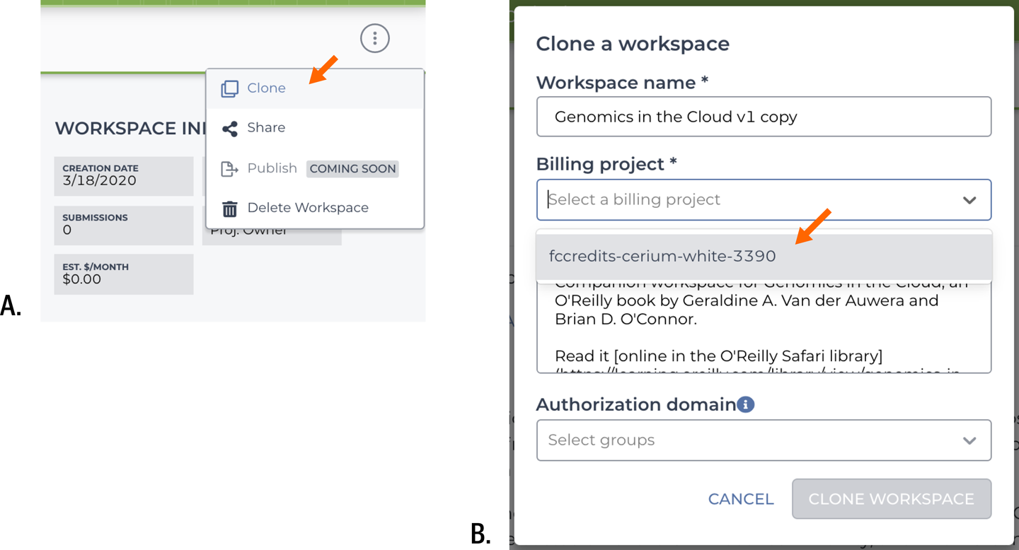
Figure 11-8. Cloning the preconfigured workspace. A) List of available actions; B) cloning form.
Select your billing project; that will determine the account GCP will bill when you do work that incurs costs. You can change the workspace name or leave it as is; workspace names must be unique within a billing project but do not need to be unique across all of Terra. Ignore the Authorization domain bit for now; that’s an optional whitelisting option that you don’t need at this time.
When you click the Clone Workspace button, you’re automatically taken to your new workspace. Take a good look around; everything that the light touches belongs to you. There’s a lot there, huh? Actually, you know what, don’t spend too much time looking around. Let’s keep a tight focus on our goal, which is to get you running workflows through Terra’s Cromwell server.
Running Workflows with the Cromwell Server in Terra
Alright, it’s showtime. Head on over to the Workflows section of the workspace, where you should see a list of available workflow configurations, as shown in Figure 11-9.

Figure 11-9. List of available workflow configurations.
These are two configurations for the same workflow, which you might recognize from the first part of their names, scatter-hc. That’s right, it’s your favorite parallelized HaplotypeCaller workflow. In case you’re wondering, the key difference between these two configurations is that one is designed to run on a single input sample, whereas the other can run on any arbitrary number of input samples. That sounds exciting, right? Right. But let’s focus on the simple case first.
Running a Workflow on a Single Sample
On the page that lists the workflow configurations, click the one called scatter-hc.filepaths to open the configuration page. Figure 11-10 shows the summary information, including a one-line synopsis and short description.

Figure 11-10. Viewing the workflow information summary.
In addition, the summary links to the Source of the workflow. If you follow that link, it will take you to the Broad Institute’s Methods Repository, an internal repository of workflows. Terra can also import workflows from Dockstore, as you’ll see in Chapter 13, but for this exercise, we chose to use the internal repository, which is a little easier to work with on first approach.
Back on the scatter-hc.filepaths configuration page, have a look at the SCRIPT tab, which displays the actual workflow code. Sure enough, it’s the same workflow that we’ve been using for a while.
As shown in Figure 11-11, the code display uses syntax highlighting: it colors parts of the code based on the syntax of the WDL language. It’s not possible to edit the code in this window, but the aforementioned Methods Repository includes a code editor (also with syntax highlighting), which can be quite convenient for making small tweaks without too much hassle.
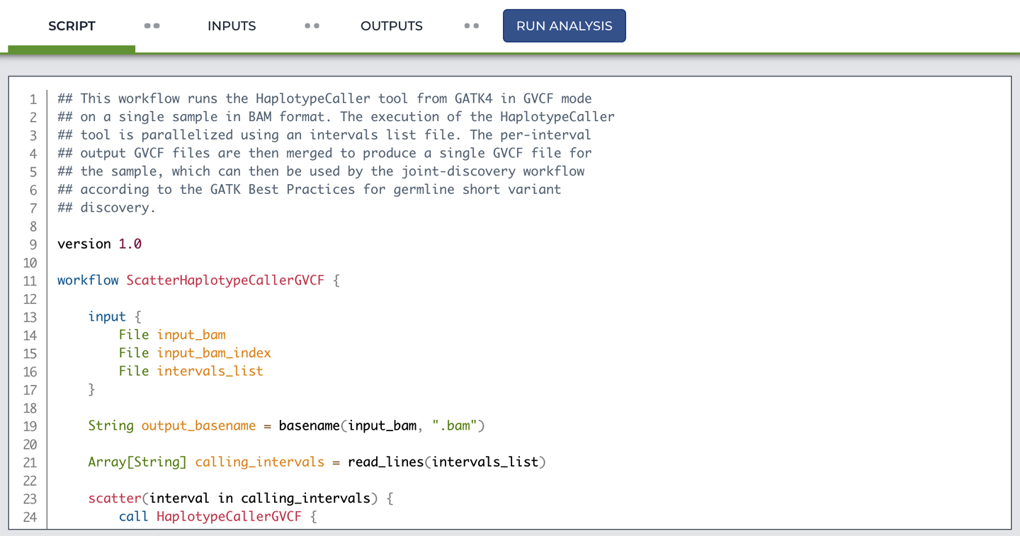
Figure 11-11. Viewing the workflow script.
So now you know for sure which workflow you’re going to be running, but where do you plug in the inputs? When you ran this workflow from the command line, you handed Cromwell a JSON file of inputs along with the WDL file. You can see the functional equivalent here on the Inputs tab, which is shown in part in Figure 11-12. For each input variable, you can see the Task name in the leftmost column and then the name of the Variable as it is defined in the workflow script as well as its Type. Finally, the rightmost column contains the Attribute, or value, that we are giving to each variable.

Figure 11-12. Viewing the workflow inputs.
We’ve prefilled the configuration form for you, so you don’t need to edit anything, but please do take a moment to look at how the input values are specified. Especially for the File variables: we’ve provided the full paths to the locations of the files in GCS. This is truly an exact transcription of the contents of the JSON file of inputs. In fact, as you’ll learn in more detail in Chapter 12, all we had to do to set this up was to upload the JSON file to populate the contents of the form.
So are you ready to click that big blue Run Analysis button? Go for it; you’ve earned it. A small window will pop up asking for confirmation, as shown in Figure 11-13. Press the blue Launch button and sit back while Terra processes your workflow submission.
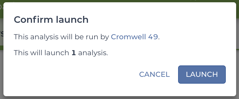
Figure 11-13. The workflow launch dialog.
Under the hood, the system sends the built-in Cromwell server a packet of information containing the workflow code and inputs. As usual, Cromwell parses the workflow and starts dispatching individual jobs to PAPI for execution on the Google Compute Engine (GCE), as illustrated in Figure 11-14.
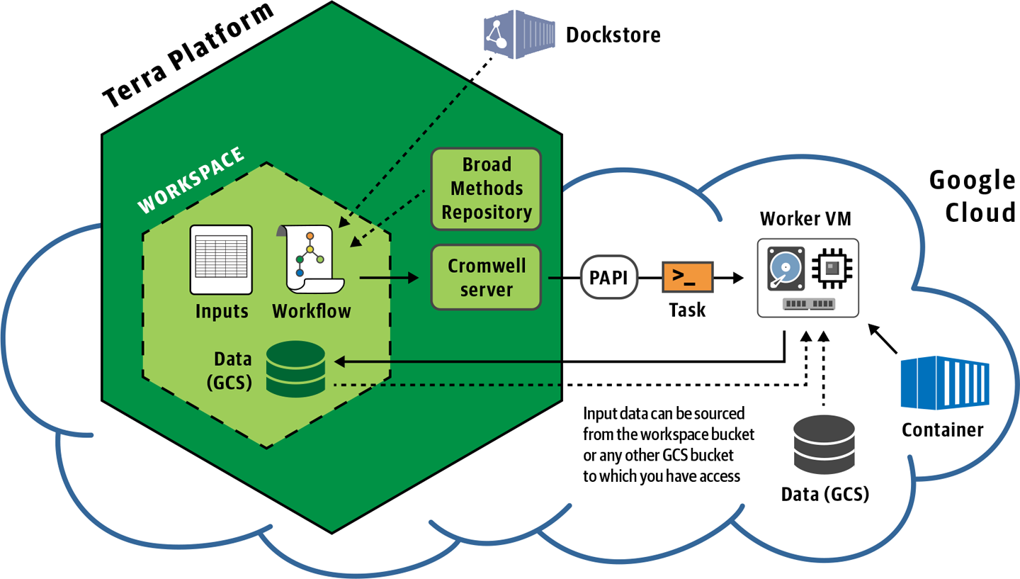
Figure 11-14. Overview of workflow submission in Terra.
Meanwhile, Terra will take you to the Job History section of the workspace, where you can monitor execution and look up the status of any past submissions—after you’ve had a chance to run some, that is. Speaking of which, there will be more to look at here when the workflow you just submitted is further along, so let’s move on and plan to circle back to the Job History later in the chapter.
At this point, assuming everything went fine, you’ve essentially just replicated your earlier achievements of running the scattered HaplotypeCaller workflow, through PAPI, on a single sample. That’s nice, but wasn’t the point that we wanted to be able to run workflows on multiple samples at the same time? Why, yes; yes, it was. That’s where the second configuration comes in.
Running a Workflow on Multiple Samples in a Data Table
Let’s go take a look at that other configuration—the one called scatter-hc.data-table. As a reminder, you need to navigate to the Workflows pane and then click the configuration. You’ll see mostly the same thing as with the previous one (and the Source link is exactly the same), but if you look closely, there is one important difference. As shown in Figure 11-15, this configuration is set up to “Run workflow(s) with inputs defined by data table,” whereas the .filepaths configuration was set to “Run workflow with inputs defined by file paths” and specified the book_sample table as the source of data, as shown in Figure 11-10.

Figure 11-15. The second workflow is set to run on rows in a data table.
Now take a closer look at how the inputs are defined on the Inputs tab. Do you see anything unfamiliar? For most of the variables, the straightforward values (like the Docker address and the file paths) have been replaced by what looks like more variables: either workspace.* or this.*, as shown in Figure 11-16.
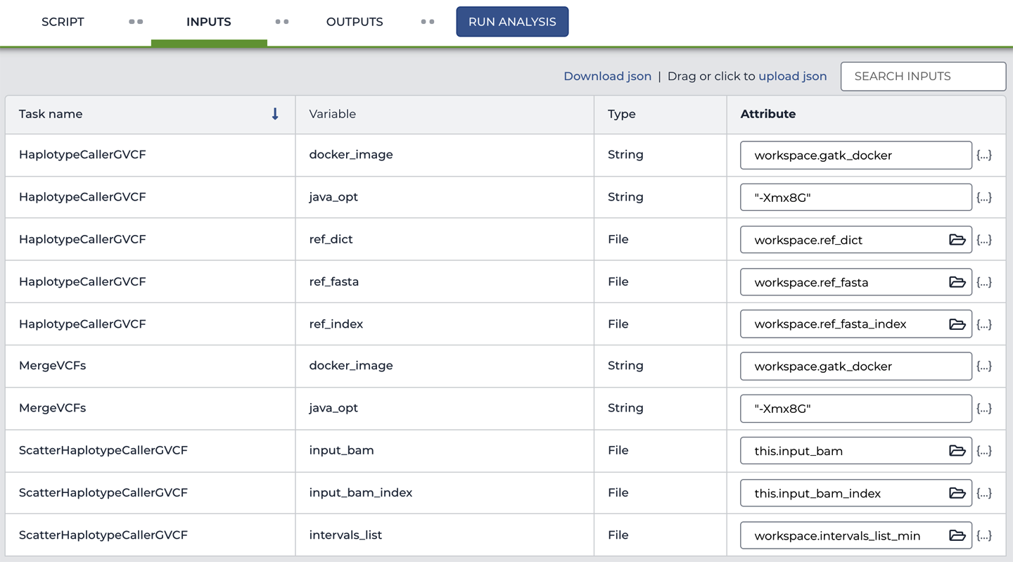
Figure 11-16. The workflow input configuration references data tables.
And that’s exactly what those are, references to values that are defined somewhere else. Specifically, they point to values that are stored in metadata tables in the Data section of the workspace. Let’s head over there now and see if we can shed some light on how this all works.
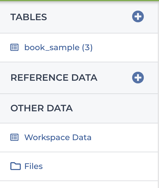
In the Data section, you’ll find a menu of data resources that should look something like Figure 11-17. Within that menu, you should see a table called book_sample and another one called Workspace Data. We’re going to start with the Workspace Data table, on the assumption that it’s the least complicated to understand.
Click Workspace Data to view the contents of that table, which are shown in Figure 11-18. As you can see, this is a fairly simple list of key:value pairs; for example, the key gatk_docker is associated with the value us.gcr.io/broad-gatk/gatk:4.1.3.0. Meanwhile, behind the scenes, this Workspace Data table is called workspace. As a result, we can use the expression workspace.gatk_docker in the workflow inputs form, as shown in Figure 11-16, to refer to the value us.gcr.io/broad-gatk/gatk:4.1.3.0, which is stored under the gatk_docker key in the workspace table.
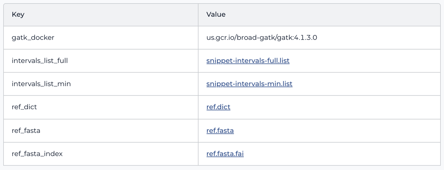
Figure 11-18. The Workspace Data table.
So the workspace keys are essentially serving as a kind of global variable that you can use in multiple configurations within the same workspace. This is very convenient if you want to update the version of the GATK Docker image in all of your configurations with minimum hassle: just update the key’s value in the Workspace Data table and you’re all set.
The same benefit applies to the resource files that are typically used in multiple workflows across a project, such as the reference genome files or the interval lists. Considering how awkward it can be to wrangle those long gs:// file paths, it’s a real blessing to be able to define them just once and then simply refer to them with short pointers everywhere else. The filenames shown in blue and underlined are full file paths to locations in GCS, even though the system shows only the filename.
Note
The keys defined in the Workspace Data table do not need to match the names of the variables from the WDL. We tend to standardize variable names and keys across our workflows in order to make it more obvious which ones go together, but it’s not a requirement of the system. If you wanted, you could set up a key called my_docker and provide it as workspace.my_docker to the gatk_docker variable in the workflow configuration.
Now let’s have a look at the other table, book_sample. As shown in Figure 11-19, this one is a more proper table, with multiple rows and columns. Each row is a different sample, identified by a unique (but for once, very readable) key in the book_sample_id column. Each sample has a file path under the input_bam column and another one under the input_bam_index column. If you peek at the paths, you might recognize these as the sample files of the family trio that we used in the joint calling exercise all the way back in Chapter 6 (Germline short variant analysis), when the world was new and you were still running individual command lines in your VM.

Figure 11-19. The book_sample table.
So how do we plug the contents of this table into the inputs form? Well, you just learned about the workspace.something syntax that we encountered in Figure 11-16; now it’s time to extend that lesson to elucidate the this.something syntax. In a nutshell, it’s the same idea, except now the pointer is this instead of workspace. and it’s going to point to any row of data taken from the book_sample table and submitted to the workflow system for processing, instead of pointing to the Workspace Data table.
Too abstract? Let’s use a concrete example. Imagine that you select one row from the book_sample table. That produces what is essentially a list of key:value pairs, just like the Workspace Data table:
book_sample_id		->    mother
input_bam      		->    gs://path/to/mother.bam
input_bam_index		->    gs://path/to/mother.bai
You can therefore refer to each value based on the column name, which has been reduced to a simple key by the process of isolating that one row. That is what the this.input_bam syntax does. It instructs the system: for every sample row that you run the workflow on, use this row’s input_bam value as an input for the input_bam variable, and so on for every variable where we use this syntax. (And again, the fact that the names match is not a requirement, though we do it intentionally for consistency.)
Alright, that was a long explanation, but we know this system trips up a lot of newcomers to Terra, so hopefully it’s been worth it. The feature itself certainly is, because it’s going to allow you to launch workflows on arbitrary numbers of samples at the click of a button. If that weren’t enough, the data table system has another benefit: when you have your workflow wired up to use the data table as input, you can start the process directly from the data table itself.
How would you like to try it out? Go ahead and use the checkboxes to select two of the samples, as shown in Figure 11-20.
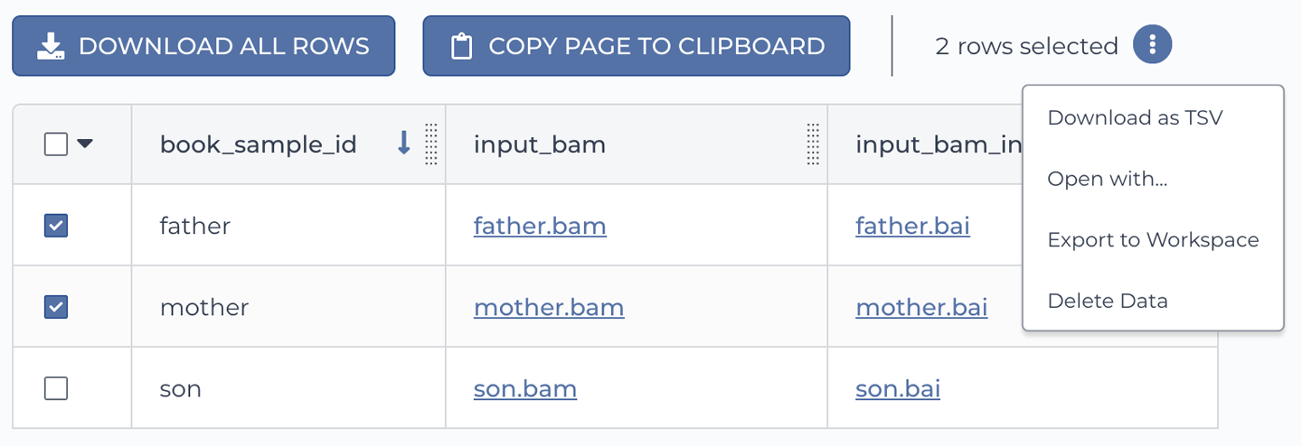
Figure 11-20. Initiating an analysis directly on a subset of data.
Having selected the samples, click the round symbol with three vertical dots located next to the count of selected rows. Click “Open with…” to open the menu of options and select Workflow as shown in Figure 11-21. Options that are not suitable for your data selection are grayed out. When you click Workflow, you’re presented with a list of available workflow configurations. Be sure to pick the one that is set up to use the data table; the system does not automatically filter out workflows that are configured with direct file paths.
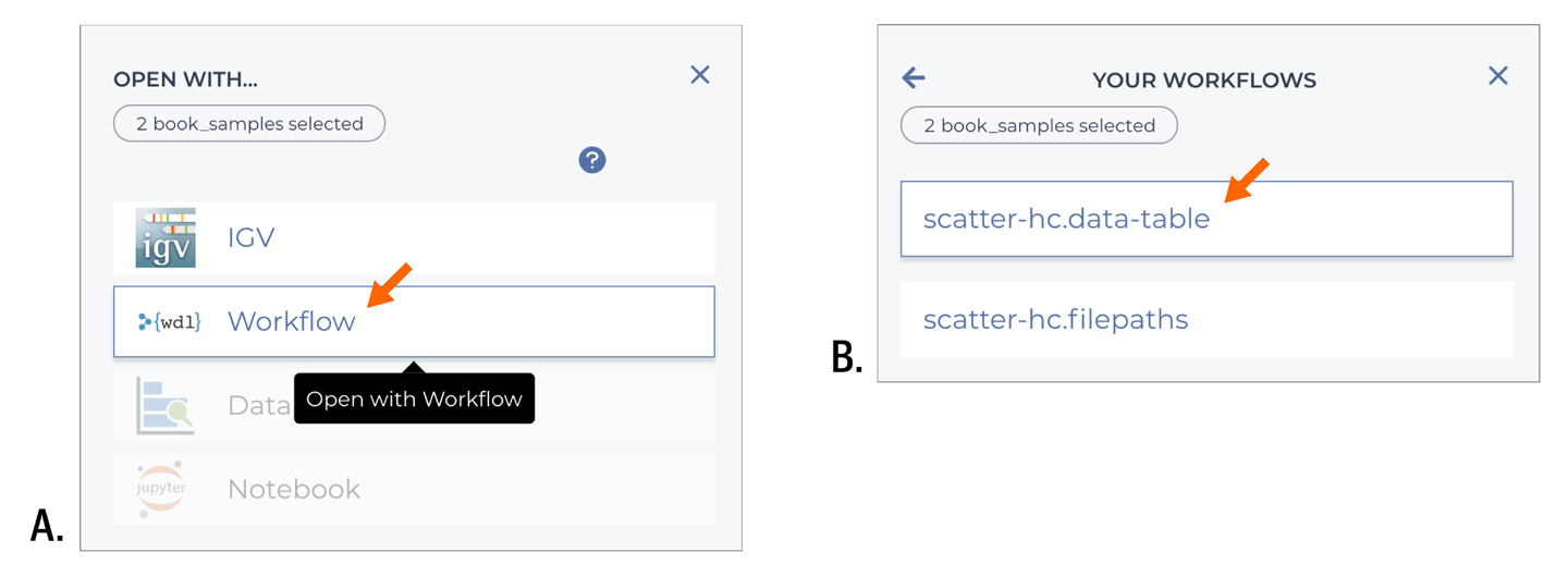
Figure 11-21. Specifying a workflow to run on the selected data.
After you pick a workflow configuration, you are brought back in the workflows section. Looking at the configuration summary, you’ll see that it’s now set to run on the subset of data that you selected, as shown in Figure 11-22.

Figure 11-22. Configuration updated with data selection.
When you submit this workflow execution request for the first time, the system saves a list of the samples you selected and stores the list as a row in a new data table called sample_set. After that, the system will add rows to the sample_set table every time you run a workflow on samples in this way. Note that you can also create sample sets yourself; you’ll see an example of that in Chapter 13.
Note
Selecting rows manually is something that we mostly do for testing purposes; it wouldn’t scale terribly well. For a more scalable approach, you can opt to run the workflow on all rows in a table, or you can create sets ahead of time. To access these options, simply click the Select Data link adjacent to the table selection menu. Speaking of which: yes, you can have multiple data tables in a workspace, although you cannot launch a workflow on multiple tables at the same time.
Finally, there’s nothing left to do but click the Run Analysis button and then confirm the launch. But this time, when you land in the Job History section, stick around so that we can take a look at how your first workflow submission fared.
Monitoring Workflow Execution
When you’re taken to the Job History page after launching a workflow, what you see is the summary page for the submission you just created. If you wandered off in the meantime and then came back to the Job History page on your own steam, what you’ll see is a list of submissions, as shown in Figure 11-23. If so, you’ll need to click one of them to open it in order to follow the instructions that follow.

Figure 11-23. List of submissions in the Job History.
The submission summary page, shown in Figure 11-24, includes a link back to the workflow configuration, information about the data that the workflow was launched on, and a table listing individual workflow executions.
Each row in the table corresponds to an individual run of the workflow. If you used the data table approach to launch the workflow, the Data Entity column shows the identifier of the corresponding row in the data table as well as the name of the table. If you ran the workflow directly on file paths, as we did in the first exercise, that column is left blank. The Workflow ID is a unique tracking number assigned by the system and links to the location of the execution logs in GCS; if you click it, it will take you to the GCP console. Most of the time, you’ll want to ignore that link and use the View link instead, in the leftmost column, to view detailed status information about the workflow run.
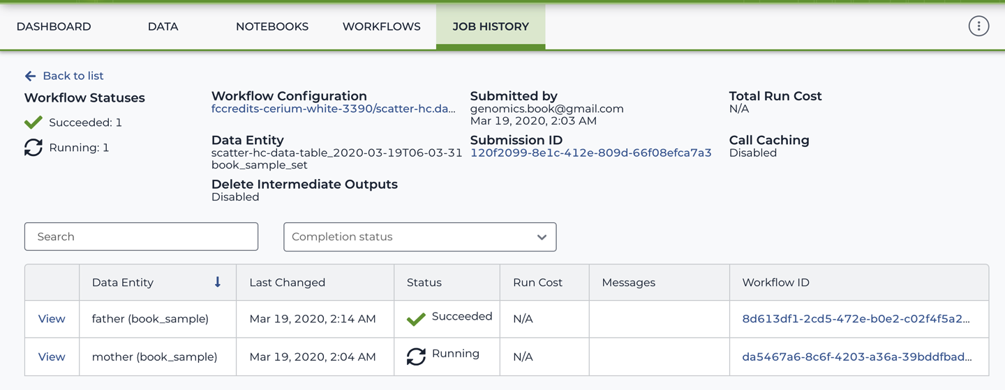
Figure 11-24. The workflow submission summary page.
Go ahead and click the View link in one of the rows to open up the details for that workflow run. The workflow run details page packs in a lot of information, so let’s go through it one piece at a time.
Note
As of this writing, the workflow run details open on a new page titled Job Manager because it uses a service that is not yet fully integrated into the main Terra portal. You might need to sign in with your Google credentials to access the workflow run details page.
First, have a look at the overall status summary pane, shown in Figure 11-25. If everything goes well, you’ll see your workflow change from Running to Succeeded

Figure 11-25. Workflow in A) Running state and, B) Succeeded state.
In the unfortunate event that your workflow run failed, the page will display additional details, including any error messages and links to logs, as shown in Figure 11-26.
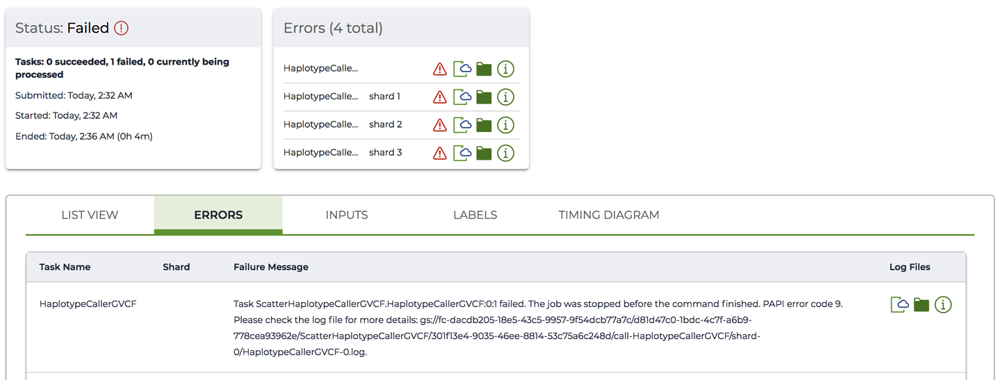
Figure 11-26. A workflow in Failed state with ERRORS summary and Failure Message.
When everything’s working, the panel below the summary pane, shown in Figure 11-27, is your go-to for everything you need to monitor the step-by-step execution of your workflow. The list of tasks will be updated as the workflow progresses and will be populated with useful resources like links to each task’s logs, execution directory, inputs, and outputs. To be clear, tasks won’t be listed until the work on them actually starts, so don’t panic when you see only a subset of the tasks in your workflow if you check on its status while it’s still running.
You might notice that in Figure 11-27, the HaplotypeCallerGVCF task is represented a bit differently compared to the MergeVCFs task: its name is underlined and there is a symbol on the side that looks like a stack of paper. This is how scattered tasks are represented. As shown in Figure 11-28, you can hover over the stack symbol to see a status summary for all of the shards generated at that step; that is, the individual tasks resulting from the scatter.
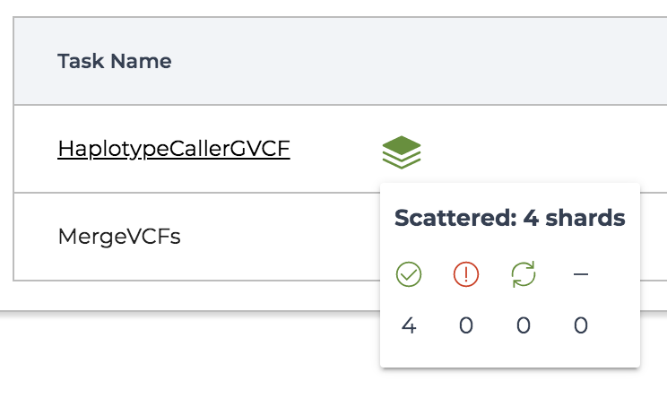
Figure 11-28. Viewing the status of shards for a scattered task.
The panel shown in Figure 11-27 has multiple tabs, so take a minute to explore those, as well. Our favorite tab in this panel is Timing Diagram, shown in Figure 11-29, which shows you how much time each task took to run. This includes not just the time spent in the User Action stage—running the analysis command (for example, HaplotypeCaller), but also the time spent on getting the VM set up, pulling the container image, localizing files, and so on.

Figure 11-29. A timing diagram showing the breakdown of runtime per stage of execution for each task call.
If you recall the discussion about workflow efficiency in Chapter 10, some amount of overhead is associated with each stage. The timing diagram is a great resource for examining this. It can help you identify any bottlenecks in your workflow that you need to address; for example, if your list of genomic intervals is not well balanced or if a particular command is taking far more time than it should.
Want to see it in action? Try hovering your mouse over the colored segments, and you’ll see tooltips appear that indicate the stage you’re looking at and the amount of time it took. For example, in Figure 11-29, we were looking at the yellow block on the right side, which shows that HaplotypeCaller took just 21 seconds to run on the very short interval we gave it for testing purposes. In comparison, it took 101 seconds to pull the container image!
Finally, you might notice that the name of the task in the pop-up window includes attempt 1. This is because the workflow is configured to use preemptible instances, which we also discussed in the section on optimizations in Chapter 10. If one of your tasks is preempted and restarted, each run attempt will be represented by a separate line in the diagram, as shown in Figure 11-30 (which comes from an unrelated workflow that we ran separately).
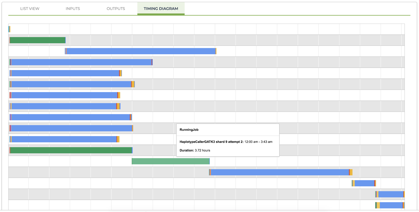
Figure 11-30. A timing diagram showing preempted calls (green bars, at lines 2, 12, and 13 from the top).
The bars representing preempted jobs are displayed in a single solid color because the different stages of operation are not reported. As a result, you can usually see fairly clearly whether a pattern of serial preemptions exists; for example, in Figure 11-30 a job was started and then interrupted by preemption (line 12 from the top), restarted and interrupted again (line 13 from the top), and then restarted again and this time was successful. You can see from this example, in which even the shortest preempted job ran for almost four hours, that if you run into several preemptions in a row for a job that constitutes a bottleneck in your pipeline, the overall runtime can increase dramatically as a result. This highlights the importance of evaluating carefully whether the cost savings that you can reap from using preemptible instances is worth the risk of your pipelines taking much longer to complete. Our rule of thumb is that if our large-scale data-processing results are due next week, bring on the preemptibles. But if we’re frantically trying to finish a demo for a conference in two days, turn them off and suck up the extra cost.
Locating Workflow Outputs in the Data Table
As we noted earlier, the workflow details shown in Figure 11-27 include pointers to the location of output files. That’s a pretty decent way to locate outputs for a particular workflow run, but that’s not going to scale well when you’re working on hundreds or thousands of samples. Not to mention hundreds of thousands of samples. (Yep, some people are at that point—isn’t it an exciting time to be alive?)
There is a much better way to do it if you used the data table, which you would need to do if you’re working at that scale. Here it is: with a tiny configuration trick, you can get the system to automatically add the workflow outputs to the data table. And, of course, we enabled that in the workflow configuration we made you run, so let’s go have a look at the data table, shown in Figure 11-31, to see whether it worked.

Figure 11-31. The data table showing the newly generated output_gvcf column.
And there it is! As you can see in Figure 11-31, a new column has appeared in the book_sample table, named output_gvcf, and all the samples we ran the workflow on now have file paths corresponding to the GVCFs produced by the workflow runs.
So, where does the name of the new column come from? Let’s return to the scatter-hc.data-table workflow configuration and take a look at the Output tab, which we ignored earlier. As you can see in Figure 11-32, we specified the output name and set it to be attached to the row data using the this. syntax, which we described earlier. You can pick an arbitrary name (for example, you could instead use this.my_gvcf), or you can click “Use defaults” to automatically use the name of the variable as it is specified in the workflow script, as we did here.
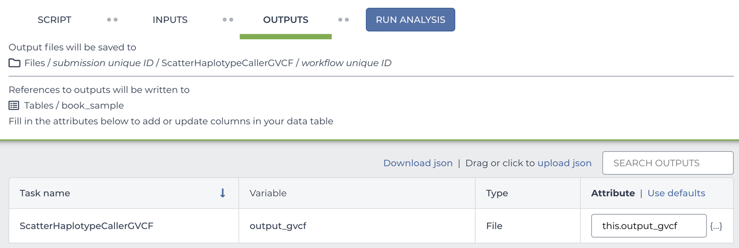
Figure 11-32. The workflow outputs configuration panel.
Keep in mind that this option is available only if you’re using the data table to define the workflow inputs. In either case, however, the location where the files are written is the same. By default, the system stores all outputs produced by workflows in a bucket that is tightly associated with the workspace. The bucket is created automatically when you create a workspace, and it has the same ownership permissions as the workspace, so if you share the workspace with someone (same menu as for cloning), they will also be able to access the data in your workspace. One important restriction, however, is that you cannot modify the bucket’s permissions outside of Terra.
Note
If you delete a workspace, its bucket will also be deleted, along with all its contents. In addition, when you clone a workspace, the data is not copied, and any paths in metadata tables will continue to point to the data’s original location. This is great because it allows you to avoid paying storage fees for multiple copies of the same data that you would otherwise generate. But if you thought you could save a copy of your data by cloning a workspace before deleting the original, well, you can’t.
Finally, you might have noticed on the Data page that there is a Files link in the lefthand menu, which is visible in Figure 11-31 among others. If you go back to that page and click the Files link, it will open a filesystem-like interface that you can use to browse the contents of the bucket without having to leave Terra, as shown in Figure 11-33.

Figure 11-33. The file browser interface showing workflow outputs in the workspace bucket.
You can even add files to your bucket by dragging and dropping them from your desktop into the file browser. That being said, if you prefer, you can always access the bucket through the GCS console and interact with its contents through gsutil.
Running the Same Workflow Again to Demonstrate Call Caching
Did you think we were done? Not quite; we couldn’t possibly let you move on without experiencing the wonder that is Cromwell’s call caching feature. We’ve already gone over its purpose several times—make it so you can avoid running duplicate jobs, and resume a workflow from the last point of failure, interruption or modification—so now let’s see it in action. Go ahead and use the launching process you just learned to run the workflow again on one of the samples that you already ran on earlier. When you land on the Job History page, click through to the workflow monitoring details when the View link becomes available. It might take a couple of minutes, so feel free to go grab yourself a cup of tea, coffee, or other beverage of choice—just don’t spill it on your laptop when you return. And remember to refresh the page; the workflow status doesn’t refresh on its own.
When you’re on the workflow details page, navigate to the Timing Diagram and hover over the widest bar for one of the lines. You should see something like Figure 11-34, reporting on a stage named CallCacheReading that took about 10 seconds to run.

Figure 11-34. A timing diagram showing CallCacheReading stage run time.
If you hover over the other bars, you’ll also see that you can’t find any of the stages related to pulling the container image or localizing inputs. This shows you that when call caching kicks in for a task, the system doesn’t even go to the trouble of setting up VMs. In fact, Cromwell doesn’t even dispatch anything about that task to PAPI.
So what exactly does happen? Good question; let’s talk about how call caching works in practice. First, you should know that whenever the Cromwell server runs a task call successfully, it stores a detailed record of that call in its database. This includes the name of the task and all of its input values: files, parameters, container image version, everything—as well as a link to the output file. Then, the next time you send it a workflow to run, it will check each task against its database of past calls before sending it out for execution. If it finds any perfect matches, it will skip execution for that task and simply output a copy of the output file that it had linked to in the last successful execution. Figure 11-35 illustrates this process.

Figure 11-35. Overview of Cromwell’s call caching mechanism.
In this example, all task calls in the workflow matched the call cache; in other words, call-cached (yep, you can use it as a verb), so nothing actually was run except a few file copying operations done by the Cromwell server itself. If you were to modify the MergeVCFs call even slightly and run this again, the HaplotypeCaller calls would call-cache, but MergeVCFs would not, so Cromwell would send that call to PAPI for execution. You can try this out by changing the version of the container image used by MergeVCFs (try 4.1.4.1) and then have a look at the Timing Diagram.
Note
You can disable call caching by clearing the checkbox in the workflow configuration, but why would you even want to do that? Call caching is fantastic. Call...ka-ching! (Because it saves you money.) #dadjokes.
Alright, time to take a break. How are you feeling? It’s normal to feel a little light-headed at this point; after all, you just got superpowers. Seriously, you are now capable of running real, sophisticated genomics workflows on as many samples as you can get your hands on. That’s no small feat. Yet the proof, as they say, is in the pudding, so grab a spoon and let’s go bite off something big.
Running a Real GATK Best Practices Pipeline at Full Scale
Do you remember Mystery Workflow #2 from Chapter 9, which turned out to be the Broad Institute’s whole genome analysis pipeline? It’s probably not the biggest genomics pipeline in the world (though it is plenty big), and it’s not the fastest pipeline in the world either (because it needs to be inexpensive). But it might just be the pipeline that has processed the largest number of human whole genome samples in the history of genomics (so far). If you’re looking to learn how to do something fairly standard that will come in handy at some point in the future, this pipeline would be a reasonable choice.
In this last section of the chapter, we’re going to show you where to find it, test it, and run it on a full-scale human whole genome sample.
The good news is that it’s going to be pretty straightforward. We already mentioned previously that the GATK team makes its Best Practices workflows available in a GitHub repository, but that’s not all; it also provides fully loaded Terra workspaces for all of them. These Best Practices workspaces contain data tables populated with appropriate example data samples (typically a small one and a full-scale one), and workflow configurations that are already wired up to run on the example data. All you need to do is clone the workspace. Then, you can follow the procedure that you learned in this chapter to run the workflows right out of the box. (We show you how to bring in data from other sources in Chapter 13.)
Finding and Cloning the GATK Best Practices Workspace for Germline Short Variant Discovery
You already visited the Terra Library showcase earlier in this chapter to find the tutorial workspace we created for the book. Let’s go back there, but this time you’re going to look for an actual Best Practices workspace published by the GATK team. As of this writing, the featured germline short variants workspace is called Whole-Genome-Analysis-Pipeline, as shown in Figure 11-36. This name might change in the future because the team has plans to adapt how they name and package these resources in light of the expanding scope covered by its tools. If you’re having trouble finding the right workspace, check the GATK website’s Best Practices section, which hosts a list of relevant resources that includes the Terra workspaces. Be sure to also check our book’s blog, where we’ll provide updates over time.
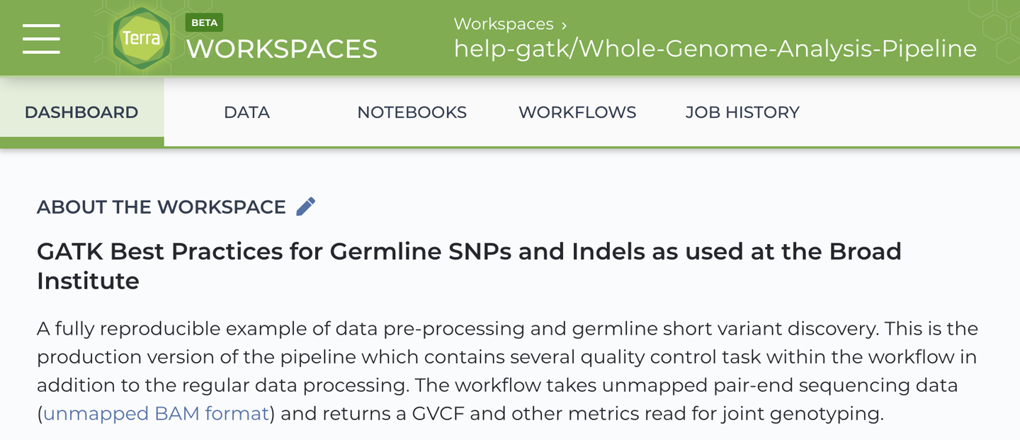
Figure 11-36. Summary information for the Whole-Genome-Analysis-Pipeline workspace.
When you’ve found the workspace, clone it as described earlier in this chapter. You’ll notice that the Dashboard provides a lot of information about the workflow, the example data and how to use these resources effectively. It even includes a summary of how long it takes and how much it costs to run the workflow on the various samples in the example data table. Speaking of which, let’s go see what’s in there.
Examining the Preloaded Data
In your clone workspace, navigate to the Data section. Again, this might change, but as of this writing, this workspace contains two main data tables as well as the Workspace Data table. The latter lists the full-scale version of the genome reference files and other resources used in the whole genome pipeline. Note that these resources are all based on the hg38 build (more properly known as GRCh38) and would therefore not be compatible with the data in the tutorial workspace that we were using earlier.
The two main data tables are called participant and sample, as shown in Figure 11-37.

Figure 11-37. A list of tables and detailed view of the sample table.
The sample table should look familiar to you because it’s the same kind of table as the book_sample table that you encountered earlier in this chapter, with a few additional columns. As you can see in Figure 11-36, two samples are listed there: NA12878 and NAA12878_small. They both originate from the same study participant, dubbed NA12878. The former is a full-size whole genome sequencing dataset, whereas the latter is a downsampled version of that dataset. For each sample, we have a list of unmapped BAM files (which will be the main input to the workflow) as well as other files that the documentation explains are outputs produced by the workflow, which has already been run in this workspace.
The participant table, on the other hand, is probably new to you. It lists the study participants, though in this case, that’s just a single person. If you looked carefully at the sample table, you might have noticed that one of its columns is participant, which is an identifier that points to an entry in the participant table (participant_id in that table). The purpose of the participant table is to provide a higher level of organization for your data, which is useful when you have multiple study participants, and each of them can have multiple samples associated with them, either corresponding to different data types, different assays, or both. With this setup, you can use the data table system to do things like run a workflow on all the samples that belong to a subset of participants, for example.
As another example, the Mutect2 somatic analysis pipeline (described in detail in Chapter 7) expects to see a tumor sample and a matched normal sample from each patient, which are formally described as pairs of samples. If you check out the corresponding GATK Best Practices workspace (this one, at the time of writing), you’ll see it has four data tables organizing the data into participants, samples, pairs of samples, and sets of samples (for the normals that are used in the PoN, described in Chapter 7). The data tables in that workspace conform to a data model defined by the TCGA cancer research program: The Cancer Genome Atlas.
More generally, you can use any number of tables to organize your data and describe the relationships between data entities like participants, samples, and others in a structured data model. In Chapter 13, we discuss options for building your data model in Terra and using it effectively to save yourself time and effort.
Selecting Data and Configuring the Full-Scale Workflow
As we’ve described previously, you can either head straight for the workflows page in the workspace or you can start the process from the Data page by selecting one or both samples in the sample table. (We recommend selecting both so you can experience the runtime difference of the plumbing test and the full-scale run for yourself.) If you choose to follow the same procedure as previously, click “Open with…” to choose the workflow option, and select the one workflow that is preconfigured in this workspace. Unless a lot has changed since the book came out, this should be the same, or practically the same, as the workflow that we examined in detail in Chapter 9. However, you’ll notice that on the workflow page, you can view only the main WDL script, not any of the additional WDL files that contain the subworkflows and task libraries. This is a limitation of the current interface that will be addressed in future work.
We didn’t look at the inputs to this workflow in much detail when we dissected it in Chapter 9, because at the time we were focused on understanding its internal plumbing. Now that we’re looking at them through the Terra interface, in the context of the workflow inputs configuration form, it’s pretty striking that it seems to have only four required inputs, which is fewer than the much simpler workflow we’ve been working with so far. However, this is mostly a distortion of reality; in fact, two of those four inputs represent a larger number of inputs that are bundled together using struct variables, which we encountered in Chapter 9. These two structs represent the two most typical categories of inputs that you will frequently encounter in genomics workflows. One is a bundle of reference data, grouping the genome reference sequence, associated index files, and known variant resources for validation. The other groups the files that hold the actual data that you’re looking to process.
Most of the optional inputs to this workflow are task-level runtime parameters and conditional checks, which are readily recognized by their type, Boolean. You might recall that in the first workflow we examined in Chapter 9, we found a lot of conditional statements that defined settings like default runtime resource allocation. The optional inputs we see here are set up so that you can override those default settings when you configure the workflow; for example, if you have reason to believe that the defaults won’t be appropriate for your use case. Yet if you don’t know the first thing about what the runtime resource allocations should be, you can just leave those fields blank and trust that the presets will be good enough.
It’s also worth taking a quick peek at the Output tab, where you’ll be reminded that this workflow produces a ginormous number of outputs, which are mostly quality control-related metrics and reports. This is where we really appreciate being able to have the paths to the output files written to the data tables, which makes it a lot easier to find outputs than if you had to go rooting around in the Cromwell execution directories for each file. For the record, the outputs that you’re most likely to care about are the trio of output_bam, output_cram, and above all, output_vcf, which is the set of variant calls that you’ll want to use in downstream analysis.
That being said, all of this should mostly be prefilled and ready to go, but on the Output tab, click “Use defaults” to set up the mapping of outputs to the sample table.
Launching the Full-Scale Workflow and Monitoring Execution
Enough talk, let’s run this thing! As previously, click Run Analysis and then Launch to submit the workflow for execution. You can follow the same steps as we described earlier to monitor the progress of your pipeline, but you should expect this to take quite a bit longer! As mentioned earlier, the Dashboard summary includes typical runtimes for the workflow running on both example datasets, so be sure to use that as a guide to gauge when to go check how it’s going. You can also browse the Job History of the original workspace (the one you cloned your copy from); it includes past executions, so you can look up the timing diagram there.
One new thing you might notice is that the List view of the workflow details page collapses subworkflows and displays their name in underlined font, as shown in Figure 11-38. This is similar to the representation of scattered tasks but lacks the little stack icon on the side.
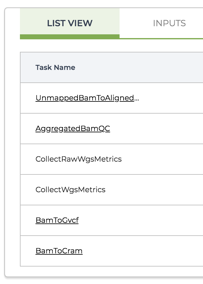
Figure 11-38. The List View of the task calls in the master workflow.
Have a look at the timing diagram provided at this level: you essentially get a high-level summary of the component segments of the workflow, as shown in Figure 11-39. If you hover over the various lines, you’ll see that the longest segment on the left corresponds to UnmappedBamToAlignedBam, the data processing subworkflow that takes in the raw unmapped data and outputs an analysis-ready BAM file. The next three lines consist of the main quality control subworkflow, AggregatedBamQC, and two metrics collection tasks that are not bundled into subworkflows. Next down is the BamToGvcf variant-calling subworkflow, which produces the final output of the per-ample pipeline, the GVCF file of variants. You’ll notice that those four segments all started at the same time, when the very first segment completed because they are independent of one another. This is parallelism in action! Finally, the last segment is the BamToCram workflow, which produces a CRAM file version of the processed sequencing data for archival purposes. The timing of that one might seem odd until you realize that it starts immediately after the AggregatedBamQC workflow finishes.

Figure 11-39. The timing diagram for the master workflow showing subworkflows (solid red bars) and individual tasks that are not bundled into subworkflows (multicolor bars).
Now go back to the List View and click through one of the subworkflows; for example, the BamToGvcf variant calling subworkflow. You’ll see it open up on its own page as if it were a standalone workflow, with its own list of tasks, timing diagram, and so on, as shown in Figure 11-40.
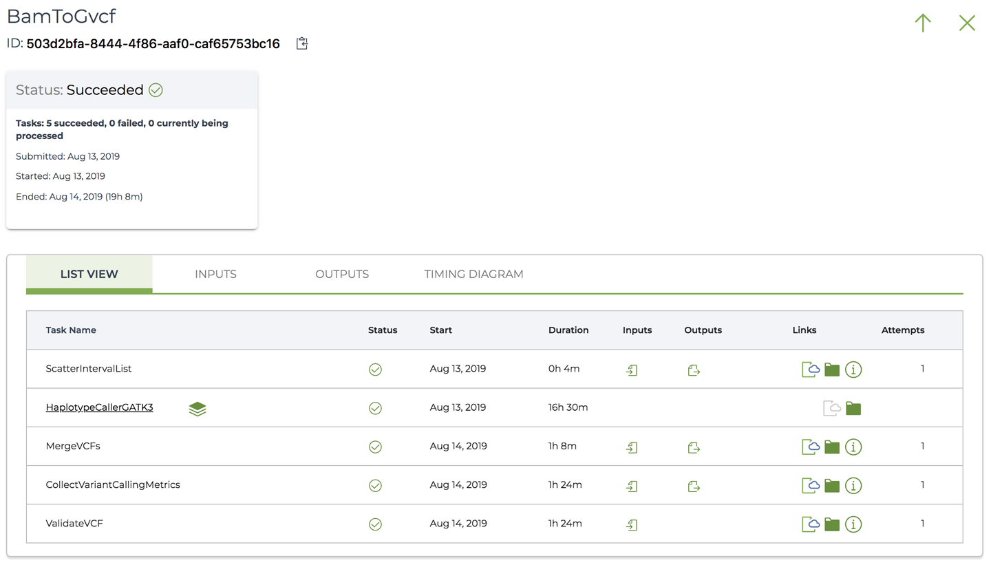
Figure 11-40. The workflow details page for the BamToGvcf subworkflow.
There is theoretically no limit to how deeply you can nest WDL subworkflows, as long as you don’t create loops. In practice, though, we have not yet seen workflows with more than three levels of nesting (including task libraries). In any case, you can navigate back up to the parent workflow level by clicking the upward-pointing arrow in the upper-right corner.
Finally, you can check that the outputs were produced as expected, both in the Job History view and in the sample data table, as we’ve described earlier in the chapter.
Options for Downloading Output Data—or Not
Whether you’re browsing the outputs of your workflow through the Job History page, or through either the data tables or the Files browser on the Data page, you can download any file by simply clicking its name or path. This brings up a small window that includes a preview of the file (if it’s in a readable text format), its size, and an estimate of the cost of the download, which is due to egress fees. In Figure 11-41, we have examples of such download windows for two kinds of files: the list of unmapped BAM files that served as input for the pipeline, which is a plain-text file and can therefore be previewed, and the GVCF that is the final data output of the pipeline, which is originally plain text, too, but here, was gzipped to require less storage space, and therefore cannot be previewed. That would also be the case for other compressed file formats like BAM and CRAM files, which also cannot be previewed.
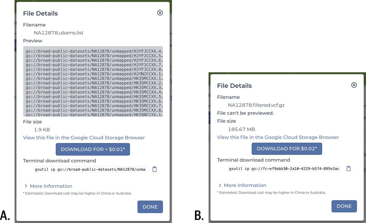
Figure 11-41. File download windows showing A) the list of unmapped BAM files, and B) the final GVCF output.
The download window offers three ways to download the file of interest. You can follow the link to the GCS console, where you can select multiple files and download them through your web browser. You can also simply click the blue Download button for that one file, which will also be downloaded by the web browser. Alternatively, you can copy the terminal download command, which includes the full path to the file’s location in GCS, to download the file with the command-line tool gsutil.
The direct download option is fine for individual files that you want to look at quickly, especially if they’re small. For example, the 1.9 KB text file in Figure 11-41 is predicted to cost less than a penny to retrieve. If you need to retrieve multiple small to medium files like the 185 MB GVCF in Figure 11-41 (just two cents? sounds reasonable), you’ll usually be better off using either the GCP console or better yet, gsutil. But if you find yourself needing to retrieve large files (many gigabytes, many dollars), it might be worth pausing to rethink whether you really can’t do what you need to do without a local copy of the file. For example, were you planning to look at the BAM and VCF files in IGV to check some variant calls by eye? Remember, you can do that by connecting IGV to GCS. Or did you want to run another kind of analysis that you don’t have a workflow for, or that requires an interactive process? Ah, that’s fair…but maybe you could continue that work in the cloud rather than falling back to a local environment. Wouldn’t it be amazing if you could do all of your work in the cloud, from the raw data all the way to making the figures that are going to be in your paper?
That is not a pipe dream. It’s already possible today—but you’re going to need something better than just the VM and something different from the workflow system. You will need an integrated environment for interactive analysis on the cloud, which Terra provides as well.
Note
The filename produced by the workflow uses a plain .vcf extension instead of .g.vcf, which is optional but recommended for signifying that a file is, in fact, a GVCF rather than a regular VCF file. This highlights the fact that you can rarely rely on filenames and extensions to know for sure what a file contains and how it was produced. Data management frameworks like the workspace data model can mitigate such problems by helping us keep track of the relationships between pieces of data.
Wrap-Up and Next Steps
For the past four chapters, including this one, we’ve been living and breathing for workflows. We started out small in Chapter 8, running canned WDL scripts on a single VM. Then, in Chapter 9 we dissected real genomics workflows to learn what they did and how they were wired up. This led us to a better understanding of some of the requirements of such workflows, which are designed to take advantage of various cloud features including parallelism and burst capability.
But that made us realize that we couldn’t continue running workflows on a single VM, even if we beefed up its resource allocations, so we moved to dispatching jobs to PAPI for execution in Chapter 10. We experimented with two approaches for doing so: directly with Cromwell and through the WDL Runner wrapper, which showed us the power of PAPI but also showed us the limitations of launching a single workflow at a time.
Finally, we moved to Terra in this chapter to use its built-in, full-featured Cromwell server. We were able to take advantage of some of the Cromwell server’s coolest features, like the vaunted call caching mechanism and the timing diagram, without worrying for a second about server maintenance. Along the way, we also encountered unexpected benefits of using Terra, mainly thanks to the integration of data management with workflow execution. Having learned to launch a workflow on rows in a data table, we’re now able to process arbitrary amounts of data without breaking a sweat. And we know how to get the outputs to be added to the table automatically, so we don’t need to go digging for them.
While explaining all this, we might have implied that applying the GATK Best Practices to your own data should now “simply” be a matter of running the workflows as demonstrated. However, in the course of a real genomic study, you’ll typically need to perform a variety of peripheral tasks that aren’t so conveniently packaged into workflows. Whether for testing commands, evaluating the quality of results, or troubleshooting errors, you’ll need to be able to interact with the data in a more immediate way. That will be even more the case if your work responsibilities extend beyond what we defined very narrowly as genomics (i.e., variant discovery) to include developing and testing hypotheses to answer specific scientific or clinical questions.
In Chapter 12, we use a popular environment for interactive analysis that also happens to do wonders for reproducible science, called Jupyter. We’ll still be working within the Terra platform, which hosts a scalable system for serving Jupyter in the cloud.
