Chapter 13. Assembling Your Own Workspace in Terra

In Chapters 11 and 12, you learned how  to use workflows and interactive notebooks in Terra using prebaked workspaces. Now, it’s time for you to learn to bake your own so you can build your own analyses within the Terra framework. This is an area provides a lot of options and multiple valid approaches, so rather than attempting to provide a one-size-fits-all path, we’re going to walk through three scenarios.

In the first scenario, we re-create the book tutorial workspace from its base components to demonstrate the key mechanisms involved in assembling a workspace from the ground up. In the second and third scenarios, we show you how to take advantage of existing workspaces to minimize the amount of work you have to do when starting a new project. In one case, we explain how to add data to an existing workspace that is already set up for a particular analysis, such as the official GATK Best Practices workspaces. In the other, we demonstrate how to build an analysis around data exported from the Terra Data Library. However, before we dive into those three scenarios, let’s explore the data management strategy that we’re applying in all three cases.

Managing Data Inside and Outside of Workspaces

One of the most important aspects of moving your work to the cloud is designing a data management strategy that will be sustainable for the long term, especially if you expect to work with large datasets that will serve as input for multiple projects. It’s a complex enough topic that a full discussion would be beyond the scope of this book, and entire books cover that subject alone. However, it’s worth taking some time to talk through a few key considerations that apply specifically in the context of Terra and shape how we decide where data should reside.

The Workspace Bucket as Data Repository

As you learned in Chapter 11, each Terra workspace is created with a dedicated GCS bucket. You can store any data that you want in the workspace bucket, and all notebooks as well as logs and outputs from workflows that you run in that workspace will be stored there.  However, there’s no obligation to store your input data in the workspace bucket. You can compute on data that resides anywhere in GCS as long as you can provide the relevant pointers to the files, assuming that you are able to grant access to that data to your Terra account (more on that in a minute).

This is important to note for a couple of reasons. First, if you’re going to use the same data as input for multiple projects, you don’t want to have to maintain copies of the data in each workspace because you’ll get charged storage costs for each bucket. Instead, you can put the data in one location and point to that location from wherever you need to use it. Second, be aware that the workspace bucket lives and dies with your workspace: if you delete the workspace, the bucket and its contents will also be deleted. Related to this, when you clone a workspace, the only bucket content that the clone inherits from its parent is the notebooks directory. The clone will inherit a copy of the parent’s data tables, retaining links to the data in the parent’s bucket, but not the files themselves. This is called making a shallow copy of the workspace contents. If you then delete the parent workspace, the links in the clone’s data tables will break, and you will no longer be able to run analyses on the affected data.

As a result, we generally recommend storing datasets in dedicated master workspaces that are kept separate from analysis workspaces, with more narrow permissions restricting the number of people authorized to modify or delete them. Alternatively, you could also store the data in buckets that you manage outside of Terra, as we did for the example data provided with this book. The advantage of storing the data outside of Terra is that you (or whoever owns the billing account for the bucket) have full administrative control over it. That gives you the freedom to do things like setting granular per-file permissions or making contents fully public, which are not currently possible in Terra workspace buckets for security reasons. It also doesn’t hurt that you can choose meaningful names for the buckets you create yourself, whereas Terra assigns long, abstract names that are not very human-friendly. However, if you decide to follow that route, you’ll need to enable Terra to access any private data that you manage yourself outside of Terra, as explained in the next section.

Accessing Private Data That You Manage Outside of Terra

So far, we’ve worked with data that’s either in public buckets or in the workspace’s own bucket, which is managed by Terra. However, you will eventually want to access data that resides in a private bucket that is not managed by Terra. At that point, you will encounter an unexpected complication: even if you own that private bucket, you will need to go through an additional authentication step that involves the GCP console and a proxy group account. Here’s what you need to know and do to get past this hurdle.

Whenever you issue an instruction to do something in GCP through a Terra service, the Terra system doesn’t actually use your individual account in its request to GCP. Instead, it uses a service account that Terra creates for you. In fact, you can have multiple service accounts created for you by Terra because you get one for each billing project to which you have access. All of your service accounts are collected into a proxy group, which Terra uses to manage your credentials to various resources. This has benefits for both security and convenience under the hood.

Most of the time, you don’t need to know about this because any resources that you create or manage within Terra (like a workspace and its bucket, or a notebook) are automatically shared with your proxy group account. In addition, whenever someone shares something with you in Terra, the same thing happens: your proxy group account is automatically included in the fun, so you can seamlessly work with those resources from within Terra. However, when you start connecting to resources that are not managed by Terra, the Google system that controls access permissions doesn’t automatically know that your proxy group account is allowed to act as your proxy. So, you need to identify your proxy group account in the Google permissions system, and specify what it should be allowed to do.

Fortunately, this is not too difficult if you know what to do, and we’re about to walk you through the process for the most common case: accessing a GCS bucket that is not controlled by Terra. For other resources, the process would be essentially the same.

First, you need to find out your proxy group account identifier. There are several ways to do that. The simplest is to look it up in your Terra user profile, where it is displayed as shown in Figure 13-1.

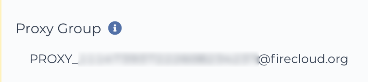
Figure 13-1. The proxy group identifier displayed in the user profile.

With that in hand, you can head over to the GCS console and look up your external bucket; that is, the bucket you originally created for the exercises in Chapter 4. Go to the Bucket details page and find the Permissions panel, which lists all accounts authorized to access the bucket in some capacity, as shown in Figure 13-2.

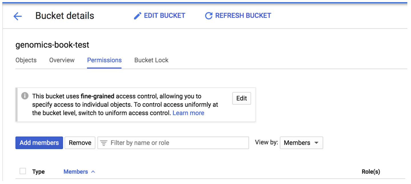
Figure 13-2. The bucket permissions panel showing accounts with access to the bucket.

Click the “Add members” button to open the relevant page and add your pet service account identifier in the “New members” field. In the “Select a role” drop-down menu, scroll if needed to select the Storage service in the left column and then further select the Storage Object Admin role in the right column, as shown in Figure 13-3. Click Save to confirm.

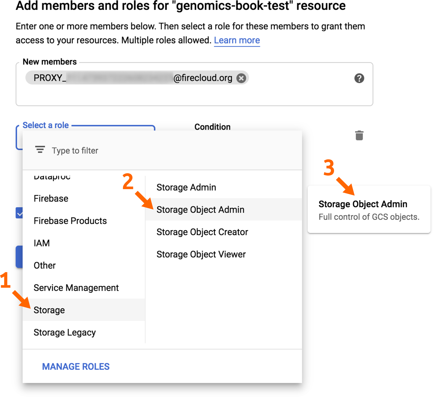
Figure 13-3. Granting access to a bucket to a new member.

After you’ve done this, you will be able to access external GCP resources such as buckets not managed by Terra from within your notebooks and workflows. For any buckets that you don’t administer yourself, you’ll need to ask an administrator to do this procedure on your behalf.

Accessing Data in the Terra Data Library

As you might recall from the context-setting discussion in Chapter 1, in which we originally introduced the platform, Terra includes a Data Library that provides connections to datasets hosted in GCP by various organizations. Some of those datasets are simply provided in Terra workspaces, like the 1000 Genomes High Coverage dataset that you’ll use in the second and third scenarios in this chapter. You’ll have the opportunity to try out a few ways to take advantage of that type of data repository.

Other datasets are hosted in independent repositories that you access through dedicated interfaces called data explorers, which enable you to select subsets of the data based on metadata properties and then export them to a regular workspace. We won’t cover those in detail but encourage you to explore the library and try retrieving data from the ENCODE or NeMo repositories, for example. Both of these are fully public and have very different interfaces, so they make for interesting navigation practice.

Exploring ENCODE and NeMo

For ENCODE, try selecting a few metadata properties to narrow the data selection. Then, look for the Export button to become active in the upper-right corner of the data explorer window. For NeMo, on the top menu bar, click the Data button, select a few properties in the menu on the left, and then go to the shopping cart icon in the upper right (interesting design choice, indeed). In the cart, click the Download options menu and select “Export to Terra.” In both cases, you’ll have the choice to create a new workspace or send the data to an existing workspace.

Most of the datasets in the Terra Data Library are restricted to authorized researchers because they contain protected health information, and the access modalities depend on the project host organization. Some, like TCGA, are mediated through dbGAP credentials, which you can link in your Terra user profile to gain automatic access if you are already authorized. Others are managed outside of Terra and require interaction with the project maintainers. If you are interested in learning more about any of the datasets in the library, click through to their project page, where you will typically find a description of access requirements.

Given the current heterogeneity of the data repositories included in the library, it is not yet trivial to use these resources effectively, especially if you intend to cross-analyze multiple datasets—which is unfortunate because that is one of the key attractions of moving to the cloud. This is an area of ongoing development, with many organizations actively collaborating to improve the level of interoperability and usability of these resources. We are already seeing early adopters successfully harness these resources in their research, and we are optimistic that upcoming improvements will make it easier for a wider range of investigators to do so as well.

For now, however, let’s dial back our ambition by a couple of notches and focus on getting the basics in place. Back to work!

Re-Creating the Tutorial Workspace from Base Components

Our most immediate goal in this chapter is to equip you with the knowledge and skills to assemble a complete yet basic workspace on your own. We’ve chosen to do this by having you re-create the tutorial workspace from Chapters 11 and 12 given that you’ve been using it extensively in previous chapters and it contains all the basic elements of a complete workspace in a fairly simple form. As we guide you through the process, we’re going to focus on the most commonly used mechanisms for pulling in the various components (data, code, etc.), and to avoid overwhelming you, we’re intentionally not going to discuss every option that is available on the platform.

Are you ready to get started? Because we’ll have you check the model workspace multiple times during the course of this section, we recommend that you open two separate browser windows (or tabs): one for the model workspace and another for the workspace that you are about to create.

Creating a New Workspace

In your second browser tab or window, navigate to the page that lists workspaces to which you have access, either by selecting Your Workspaces in the collapsible navigation menu or View Workspaces from the Terra landing page. You should see plus sign next to the Workspaces header in the top left of the page. Click that now to create a new blank workspace.

Note

By default, this page lists only private workspaces that either you have created yourself or that were shared with you under the “My workspaces” tab, excluding workspaces that are publicly accessible to everyone. You can view public workspaces by selecting one of the other workspace category tabs.

In the workspace creation dialog that pops up, give your new workspace a name and select a billing project, just as you’ve done when cloning workspaces in previous chapters. Because this is a brand-new workspace, the Name and Description fields will initially be blank. The name of your workspace must be unique within your billing project, but aside from that, you have a lot of freedom in naming, including using spaces in the name, as you can see in the example in Figure 13-4.

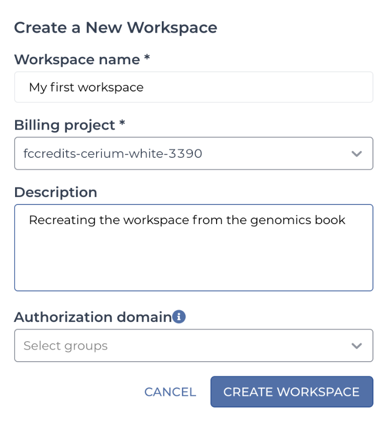
Figure 13-4. The Create a New Workspace dialog box.

The Description field is what will show up in the Dashboard of your new workspace. It’s good practice to enter something informative for future reference, even if it’s optional. You’ll have the opportunity to edit it later, though, so don’t sweat the details.

The Authorization domain field allows you to restrict access to the workspace and all its content to a specific group of users, which you must define separately. This is a useful feature for securing private information, but we’re not going to demonstrate its use here, so leave this field blank. See the article in the Terra user guide if you’re interested in learning more about this feature.

Click the Create button; you’re then directed to the Dashboard page of your brand-new workspace. Feel free to click through the various tabs to inspect the contents, but as you’ll quickly notice, there’s not much to see there, with the exception of the description you provided (if you provided one) and a link to the dedicated GCS bucket that Terra created for your workspace. You might also notice the small widget showing the estimated cost per month of the workspace, which corresponds to the cost of storing the bucket contents. That cost estimate does not include the charges resulting from the analyses you might perform in the workspace. Right now, the cost estimate is zero because there’s nothing in there. Yay?

Not that we want you to spend money, but this empty workspace is begging for some content, so let’s figure out how to load it up. Because this is supposed to be a re-creation of the tutorial from Chapter 11, we’re going to follow the same order of operations. Our first stop, therefore, will be the Workflows panel to set up the HaplotypeCaller workflow.

Adding the Workflow to the Methods Repository and Importing It into the Workspace

As you might recall, the workflow that you used in Chapter 11 was the same HaplotypeCaller workflow that you worked with in previous chapters. For the purposes of the tutorial, we had already deposited the workflow in Terra’s internal Methods Repository, so technically you could just go look it up and import it into your workspace. However, we want to empower you to bring in your own private workflows, so we’re going to have you deposit your own copy of the HaplotypeCaller WDL and import that into your workspace.

In your blank workspace, navigate to the Workflows panel and click the large box labeled “Find a workflow.” This opens a dialog that lists a selection of example workflows as well as two workflow repositories that contain additional workflows: Dockstore and the Broad Methods Repository. Click the latter to access the Methods Repository.

Expectations for Working with the Broad Methods Repository

As of this writing, the Broad Methods Repository has not yet been fully integrated into Terra and is technically considered a separate service. If that is still the case when you follow these instructions, you’ll see a blue navigation theme and references to something called FireCloud, which was the precursor to Terra and lives on as a project powered by Terra and funded by the National Cancer Institute. If you see a green theme, you live far enough in the future for the integration to be complete. We hope the planet still has ice caps and the following instructions are still valid enough to guide you successfully through the next few steps. We tried to predict what might change and minimize our dependence on screenshots, but if you find yourself stuck, check out the changelog in the book repository for updated instructions.

You may need to sign into your Google account again and accept a set of terms and conditions. Find the Create New Method button (which might be renamed to Create New Workflow) to open the workflow creation page. Provide the information as shown in Figure 13-5, substituting your own namespace, which can be your username or another identifier that is likely to be unique to you. You can get the original WDL file rom the book GitHub repository; either open the text file and copy the contents into the WDL text box, or use the “Load from file” link to upload it to the repository. By default, the optional Documentation field will be populated using the block of comment text at the top of the WDL file. The Synopsis box allows you to add a one-line summary of what the workflow does, whereas the Snapshot Comment box is intended to summarize what has changed if you upload new versions of the same workflow. You can leave the latter blank.

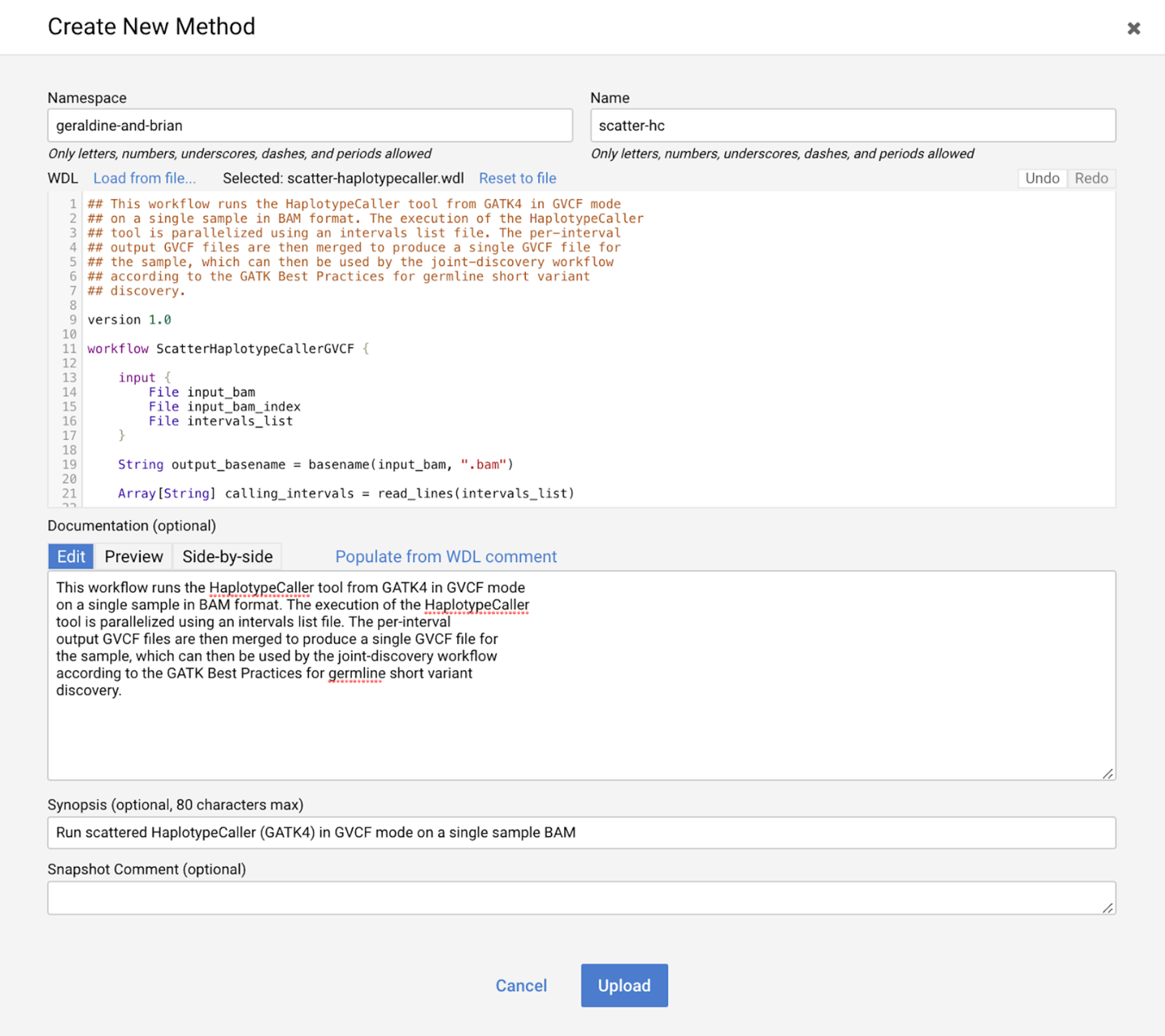
Figure 13-5. The Create New Method page in the Broad Methods Repository.

When you click the Upload button, the system validates the syntax of your WDL (using Womtool under the hood). Assuming that everything is fine, it will create a new workflow entry in the repository under the namespace you provided and present you with a summary page, as shown in Figure 13-6.

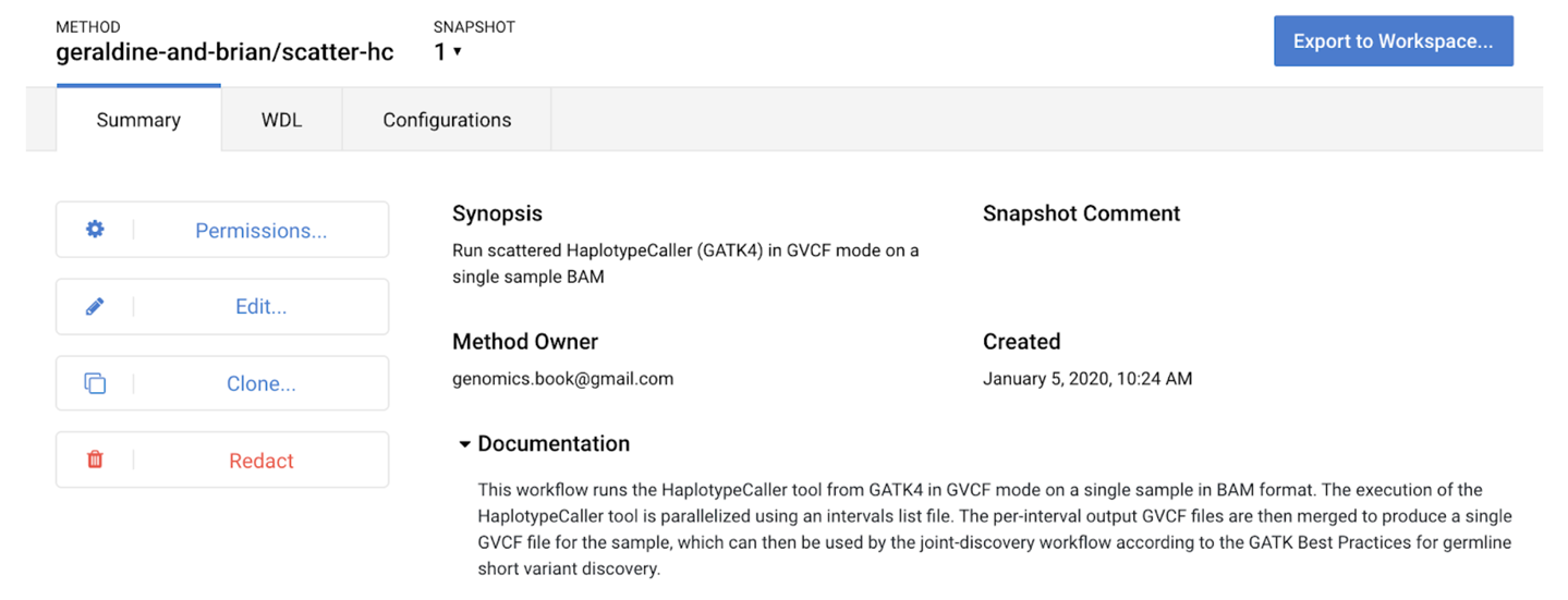
Figure 13-6. Summary page for the newly created workflow.

Take a moment to click the Permissions button, which opens a dialog that allows you to share your workflow with specific people, or make it fully public. Feel free to do either of those things as you prefer; just keep in mind that if and when you do share your workspace with others, they will be able to view and run your workflow only if you have done this. That being said, you will be able to come back to this page at a later date to do so if needed. We just bring this up now because we frequently see people run into errors after their collaborator forgot to share a workflow along with their workspace.

Incidentally, the workflow summary page is also what you would see if you had found another workflow in the Methods Repository, either by searching for it or following a link shared by a collaborator. As a result, the following instructions will apply regardless of whether you were the one who created the workflow in the first place.

Creating a Configuration Quickly with a JSON File

After you’re done sharing the workflow (or not sharing; we’re not judging), click the Export to Workspace button. If a dialog box opens prompting you to select a method configuration, click the Use Blank Configuration button. In the next dialog box prompting you to select a destination workspace, select your blank workspace in the drop-down menu and click Export to Workspace. Finally, one last dialog box might appear, asking if you want to “go to the edit page now.” Click Yes—and we swear this is the last dialog box. You should now arrive back at the Workflows page in Terra, with your brand-new workflow configuration page in front of you.

Configuring the workflow is going to be fairly straightforward. First, because we’re following the flow of Chapter 11, make sure to select the “Run workflow with inputs defined by file paths” option (located under the workflow documentation summary), which allows you to set up the workflow configuration with file paths rather than using the data tables. Then, turn your attention to the Inputs page, which should be lit up with little orange exclamation marks indicating that some inputs are missing. In fact, all of them are missing because you used a blank configuration and the workflow itself does not specify any default values.

Note

The orange exclamation marks will also show up if you have an input that is badly formatted or of the wrong variable type, like a number instead of a file. Try hovering over one of them to see the error message; all such symbols in Terra generally display me information when you hover over them and can sometimes hold the answer to your problems.

So you need to plug in the appropriate file paths and parameter values on the Inputs page. You could look up each input value individually in the original workspace and type them manually, but there’s a less tedious way to do it. Can you guess what it is? That’s right, make Jason do all the work. Er, we mean the JSON inputs file, of course. (Yes, that’s a lame joke, but if it helps you remember that you can upload a JSON file of inputs, it will have been worth the shame we’re feeling right now.)

Because we previously ran this same workflow directly through Cromwell in Chapter 10, we have a JSON file that specifies all the necessary inputs here in the book bucket. You just need to retrieve a local copy of the file and then use the “Drag or click to upload json” option on the Inputs page (right side next to the Search Inputs box) to add the input definitions it contains into your configuration. This should populate all of the fields on the page. Click the Save button and confirm that there are no longer any orange exclamation marks.

At this point, your workflow should be fully configured and ready to run. Feel free to test it by clicking the “Run analysis” button and following the rest of the procedure for monitoring execution as you did previously in Chapter 11.

With that, you have successfully imported a WDL workflow into Terra by way of the Broad Methods Repository, and configured it to run on a single sample using the direct file paths configuration option. That’s great because it means that you’re now able to take any WDL workflow you find out in the world and test it in Terra, assuming that you have the correct test data and an example JSON file available.

However, what happens when you’ve successfully tested your workflow and you want to launch it on multiple samples at once? As you learned in Chapter 11, that’s where the data table comes in. You just reproduced the first exercise in that chapter, which demonstrated that you can run a workflow using paths to the files entered directly in the inputs configuration form. However, to launch the workflow on multiple samples, you need to set up a data table that lists the samples and the corresponding file paths on the workspace’s Data page. Then, you can configure the workflow to run on rows in the data table as you did in the second exercise in that chapter. In the next section, we show you how to set up your data table.

Adding the Data Table

Remember that our tutorial workspace used an example dataset that resides in a public bucket in GCS, which we manage outside of Terra. The sample table on the Data page listed each sample, identified by a name that is unique within that table, along with the file paths to the corresponding BAM file and its associated index file, each in a column of its own.

So the question is, how do you re-create the sample data table in our blank workspace? What does Terra expect from you? In a nutshell, you need to create a load file in a plain-text format with tab-separated values. A Terra documentation article goes into more detail, but basically, it’s a spreadsheet that you save in TSV format. It’s reasonably straightforward except for a small twist that often trips people up on their first attempt: the file needs to have a header containing column names, and the first column must be the unique identifier for each row. Here’s a pro tip: rather than trying to create a load file from scratch, you can download an existing one from any workspace that has data tables and use that as a starting point. Here we’re going to be extra lazy and download the table TSV file from the original tutorial workspace, look at it and discuss a few key points, and then upload it as is to our blank workspace.

In the browser tab or window where you opened the original tutorial workspace, navigate to the Data page and click the blue Download All Rows button. This should trigger the download in your browser, and because it’s a very small text file, the transfer should complete immediately. Find the downloaded file and open it in your preferred spreadsheet editor; we’re using Google Sheets.

Note

You can also use a plain-text editor for viewing the file contents, but we recommend using a spreadsheet editor whenever you modify TSV load tables because it reduces the risk of messing up the tab-delimited format.

As you can see in Figure 13-7, this file contains the raw content from the sample data table in the original workspace, so instead of seeing just father.bam with a hyperlink, for example, we have the full path to where the BAM file resides in the storage bucket. In addition, this table has a header row that contains the names of the columns as displayed in the workspace, with one exception: the name of the first column is preceded by entity: in the file, which is not the case in the workspace. That little detail marks the most important takeaway of this whole section: the column that contains the unique identifier for each row must be the first listed in the load file, and its name must end with the _id suffix. When you upload the load file into Terra, the system will derive the name of the data table itself from the name of that column, by chopping off both the entity: prefix and _id suffix. If you don’t include a column named following that pattern, Terra will reject your table. To be clear, the name that you give to the load file has no effect on the name of the table because it will be created in Terra.

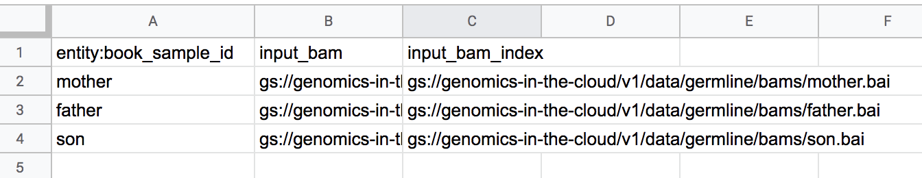
Figure 13-7. A sample data table from the tutorial workspace, viewed in Google Sheets.

Let’s try this out in practice. In your blank workspace, navigate to the Data page and click the “+” icon adjacent to TABLES on the DATA menu to bring up the TSV load file import dialog box, as shown in Figure 13-8. You can drag and drop the file or click the link to open a file browser; use either method as you prefer to upload the TSV file that we were just looking at.

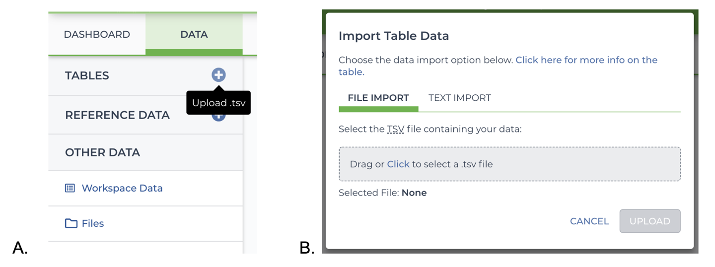
Figure 13-8. TSV load file import A) button, and B) dialog.

If the upload completes successfully, you should now see the sample table listed in the data menu. Click its name to view its content, and compare it to the original: if you didn’t make any changes, it should be identical.

Feel free to experiment with this sample load file to test the behavior of the TSV import function. For example, try modifying the name of the first column and see what happens. You can also try adding more columns with different kinds of content, like plain text, numbers, file paths, and lists of elements (use array formatting, with square brackets and commas to separate elements). And try modifying rows and creating more rows, either by adding rows to the same file or by making a new file with different rows. Just remember that if you’re editing the load file in a spreadsheet editor, as we recommend, you’ll need to make sure to save the file in TSV format.

Note

Many spreadsheet editors (including Microsoft Excel) call this format Tab-delimited Text and will save the file with a .txt extension instead of .tsv, which is absolutely fine; Terra will not care about the extension as long as the contents are formatted correctly.

If your data page ends up getting a bit messy as a result of this experimentation, don’t worry: you can delete rows or even entire tables; just select the relevant checkboxes (use the checkbox in the header to select an entire table) and click the trashcan icon that appears in the lower right of the window. The one limitation is that it’s not currently possible to delete columns from tables, so if you want to get rid of unwanted columns, you’ll need to delete the entire table and redo the upload procedure. For that reason, it can be a good idea to store versioned copies of what you consider the “good” states of your tables when you’re working on an actual project, especially if you’re planning to add data over time. There isn’t yet any built-in functionality to do that in Terra, so it’s a manual process of downloading the TSV and storing it somewhere (for example, in the workspace bucket), and in another location outside the workspace if you want to be extra cautious.

After you’re done having fun with the data tables, move on to the resource data in the Workspace Data table.

Filling in the Workspace Resource Data Table

As you might recall, the purpose of this table is to hold variables that we might want to use in multiple workflow configurations, like the genome reference sequence file, for example, or the GATK Docker container. This allows you to configure it only once, and just point to the variable in any configuration that needs it. Not only do you not need to ever look up the file path again, but if you decide to update the version or location of the file, you need to do it in only one place. That being said, you might not always want updates to be propagated to every use of a given resource file or parameter setting. When you go to set up your own analysis, be sure to think carefully about how you want to manage common resources and “default” parameters.

In practice, this data table has a very simple structure because it’s all just key:value pairs, and it comes with an easy form-like interface for adding and modifying elements. You can simply use that interface to copy over the contents of the table from the original workspace, if you don’t mind the manual process. Alternatively, you can download the contents of the original in TSV format by clicking the Download All Rows link, and upload that without modification in your workspace using the Upload TSV link. You can even drag the file from your local filesystem into the table area if you prefer. Feel free to experiment and choose the method that suits you best. With that, you’re done setting up the data, so it’s time to get back to the workflow.

Creating a Workflow Configuration That Uses the Data Tables

In your not-so-blank-anymore workspace, navigate back to the Workflows page and look at the configuration listed there, but don’t open it. Click the circle with three vertically stacked dots, which you might by now recognize as the symbol that Terra uses to provide action options for a particular asset, be it a workspace, workflow, or notebook. On the action menu that opens, select “Duplicate workflow” and then give the copy a name that will indicate that it is going to use the data table, as we did in the tutorial workspace.

Note

It’s currently not possible to simply rename a workflow configuration in place. If you want to give the “file paths” version of your workflow configuration a name that is equally explicit as we did in the tutorial workspace, you’ll need to create another duplicate with the name you want and then delete the original.

Open the copy of the configuration that you want to modify to use the data table, and this time, switch the configuration option to “Process multiple workflows.” On the drop-down menu, select the sample table and choose whether to select a subset of the data or go with the default behavior, which is to run the workflow on all items in the table. Now comes the more tedious part of this exercise, which is to connect the input assignments on the Inputs page to specific columns in the data table or variables in the workspace resource data table. Unfortunately, this time you don’t have a prefilled JSON available as a shortcut, but on the bright side, the Inputs page has an assistive autocomplete feature that speeds up the process considerably. For each variable that needs to be connected (excluding a couple of runtime parameters that we simply leave hardcoded, which you can look up in the original workspace), start typing either workspace or this in the relevant text box. This brings up a contextual menu listing all options from the relevant table: this points to whatever table you selected on the configuration’s drop-down menu, and workspace always points to the workspace resource data, which lists the reference genome sequence, Docker images, and so on.

Another way to use the assistive autocomplete feature on the Inputs page is to start typing part of the input variable name in the corresponding input text box. If the relevant data table column or workspace resource variable was set up with the same name as the input variable, as is the case in our tutorial workspace, this will typically pull up a much shorter list of matching values. For example, typing ref in one of the input fields would bring up only the workspace reference sequence, its index file, and it dictionary file. This approach can be blissfully faster when you’re dealing with a large number of variables, but it is not guaranteed to work for every configuration because it relies on the names matching well enough, which will not always be the case. Some people just want to watch the world burn.

Go ahead and fill out the Inputs page, referring to the original workspace if you become stuck at any point. When you’re done, make sure to click the Save button and confirm that there are no more exclamation marks left, as occurred previously.

What do you think, is this workflow ready to launch or what? What. Meaning, you do have one more configuration task left, which was not applicable in the “file paths” round. Pop over to the Outputs page, which requires you to indicate what you want to do with the workflow outputs. To be clear, this won’t change where the files are written; that is determined for you by the built-in Cromwell server, as you learned in Chapter 11. What this does is determine under what column name the outputs will be added to the data table. You can click the “Use defaults” link to simply use the output variable names, or you can specify something different—either a column that already exists, or a new name that the system will use to create a new column. In our workspace, we chose to use the defaults.

Considerations for Naming Outputs

Terra will happily overwrite any existing element in the table; the underlying data from any previous runs will still exist in its original location, but the link in the table will be updated to point to the latest result. To compare results from different configurations, you’ll probably want to give your outputs names that indicate which is which. Similarly, watch out for variable names that are overly generic; for example, if you have multiple workflows that produce qualitatively different outputs which are nevertheless all called output_vcf, you’re going to have a bad time.

Alright, now you’re done. Go ahead and launch the workflow to try it out and then sit back and delight in the knowledge that you’ve just leveled up in a big way. Figuring out how to use the data table effectively is generally considered one of the most challenging aspects of using Terra, and here you are. You’re not an expert yet—that will come when you master the art of using multiple linked data tables, like participants and sample sets—but you’re most of the way there. We cover that in the next scenario, in which you’ll import data from the Terra Data Library into a GATK Best Practices workspace.

Before we get to that, however, we still need to tackle the Jupyter Notebook portion of the tutorial workspace, which we used in Chapter 12. But don’t worry, it’s going to be mercifully brief—if you take the easy road, that is.

Adding the Notebook and Checking the Runtime Environment

In your increasingly well-equipped workspace, navigate to the Notebooks page, and take a guess at what should be your next step. Technically, you have a choice here. You could create a blank new notebook and re-create the original by typing in all the cells. To do that, click the box labeled Create New Notebook, and then, in the dialog that opens, give it a name and select Python 3 as the language. Then, you can work through Chapter 12 a second time, typing the commands yourself instead of just running the cells in the prebaked version as you did last time. Alternatively, you can take the easy road and simply upload a copy of the original notebook, which like everything else is available in the GitHub repository. Specifically, the cleared copy and the previously run copy of the notebook are here. Retrieve a local copy of the file and use the “Drag or Click to Add an ipynb File” option on the Notebooks page to upload it to your workspace.

Whichever road you choose to take, you don’t need to customize the runtime environment again if you created your workspace under the same billing project as the one you used to work through Chapter 12, because your runtime is the same across all workspaces within a billing project. Convenient, isn’t it? Perhaps, but it’s also a bit of a cop-out; if you were truly building this workspace from scratch, you would need to go back and follow the instructions in Chapter 12 again to customize the runtime environment. So, enjoy the opportunity to be lazy, but keep in mind that in a different context, you might still need to care about the runtime environment.

When you’re done playing with the notebook(s) in your workspace, take a step back and check that you have successfully re-created all functional aspects of the tutorial workspace. Does it all work? Well done, you! You now know all the basic mechanisms involved in assembling your own workspace from individual components.

Importing Notebooks from Outside of Terra

Speaking of different context, we’d be remiss if we didn’t address the thus-far-unspoken question: what does it take to adapt an existing notebook from a source outside of Terra? Here we’re taking advantage of importing a notebook that is already set up to use the workspace bucket and all that jazz; but what if we were just grabbing a notebook out of someone’s Binder of Python tutorials? It’s a great question, and one that you’re very likely to face in practice at some point. Again, there is no single one-size-fits-all answer, but you can use the exercises in Chapter 12 to guide you.

Review the key steps that you had to go through in the beginning that involved cloud- or Terra-specific components, like accessing data in GCS using gsutil and setting up an environment variable to easily access the workspace bucket. The steps that have to do with accessing data and saving results are typically the parts of a new-to-you notebook that you need to tweak to work smoothly in the Terra context. For the rest, the work of tweaking the runtime environment to make sure you have the right versions of software packages and libraries is very similar to what you would need to do on a local system, except in Terra you need to decide between making those tweaks from within the notebook, using a startup script, or using a custom container image (which we do not cover in detail in this book).

Documenting Your Workspace and Sharing It

The one thing you haven’t done yet to match (or outdo) the original tutorial workspace is to fill out the workspace description in the Dashboard, beyond whatever short placeholder you put in there when you created the workspace. If you have a little bit of steam left in you, we encourage you to do that now while your memory is fresh. All it takes is clicking the editing symbol that looks like a pencil on the Dashboard page, which opens up a Markdown editor that includes a graphical toolbar and a split-screen preview mode.

We don’t usually like to say anything is self-explanatory, because that kind of qualifier just makes you feel even worse if you end up struggling with the thing in question, but this one is as close as it gets to deserving that label. Take it for a spin, click all the buttons, and see what happens. Messing around with the workspace description is one of the only things you can do on the cloud that is absolutely free, and in a private clone, it’s completely harmless, so enjoy it. This is also a great opportunity to write up some notes about what you learned in the process of working through the Terra chapters, perhaps even some warnings to your future self about things you struggled with and need to watch out for.

Finally, consider sharing your workspace with a friend or colleague. To do so, click the same circle-with-dots symbol you used to clone the tutorial workspace in Chapter 11. This opens a small dialog box in which you can add their email address and set the privileges you want to give them. Click Add User and then be sure to click Save in the lower-right corner. If your intended recipient doesn’t yet have a Terra account, they will receive an email inviting them to join, along with a link to your workspace. They don’t need to have their own billing project if they just want to look at the workspace contents.

Starting from a GATK Best Practices Workspace

As you just experienced, setting up a new workspace from its base components takes a nontrivial amount of effort. Not that it’s necessarily difficult—you probably perform far more complex operations on a daily basis as part of your work—but there are a lot of little steps to follow, so until you’ve done it a bunch of times, you’ll probably need to refer to these instructions or to your own notes throughout the process.

The good news is that there are various opportunities to take shortcuts. For example, if you simply want to run the official GATK Best Practices workflows as provided in the featured workspaces by the GATK support team, you can skip an entire part of this process outright by starting from the relevant workspace. Those workspaces already contain example data and resource data as well as the workflows themselves, fully configured and ready to run. All you really need to do is clone the workspace of interest and add the data that you want to run the workflow(s) on to the data tables.

In this section, we run through that scenario so you can get a sense of what that entails in practice, the potential complications, and your options for customizing the analysis. The lessons from this scenario will generally apply beyond the GATK workspaces, to any case for which you have access to a workspace that is already populated with the basic components of an analysis. We think of this as the “just add water” scenario, which is an attractive model for tool developers to enable researchers to use their tools appropriately and with minimal effort. It’s also a promising model for boosting the computational reproducibility of published papers given that such a workspace constitutes the ultimate methods supplement. We discuss the mechanics and implications of this in more detail in Chapter 14. For now, let’s get to work on that GATK Best Practices workspace.

Cloning a GATK Best Practices Workspace

We’re going to use the Germline-SNPs-Indels-GATK4-hg38 workspace, which showcases the GATK Best Practices for short variant discovery implemented as three separate workflows. The first workflow, named 1_Processing_for_Variant_Discovery, takes in raw sequencing data and outputs an analysis BAM file for a single sample. The second, 2_HaplotypeCaller_GVCF, takes that BAM file and runs variant calling to produce a single-sample GVCF file. Finally, the third, 3_Joint_Discovery, takes multiple GVCF files and applies joint calling to produce a multisample callset for the cohort of interest.

Navigate to that workspace now and clone it as you have done previously with other workspaces. When you’re in your clone, have a quick look around to become acquainted with its contents. You’ll find a detailed description in the Dashboard, three data tables and a set of predefined resources on the Data page, and the three fully configured workflows mentioned earlier on the Workflows page.

Examining GATK Workspace Data Tables to Understand How the Data Is Structured

Let’s take a closer look at the three data tables on the Data page. One table is named participant. It contains a header line showing the name of the single column, participant_id, and a single row, populated by our beloved NA12878, or mother as we call her in this book:

participant_id

NA12878

This identifies her as a study participant; in other words, the actual person from whom biological samples were originally collected to produce the data that we will ultimately analyze.

The participant_id attribute is the unique identifier for the participant and is used to index the table. If you were to add attributes to the table (for example, some phenotype information like the participant’s height, weight, and health status), they would be added as columns to the right of the identifier.

The second table is called sample and contains multiple columns as well as two sample rows below the header. This table is more complicated than the previous one largely because in addition to the minimum inputs required to run the workflow, it contains outputs of previous runs of the workflow. Here is a minimal version of the table without those outputs:

sample_id	flowcell_unmapped_bams_list	participant _id
NA12878	NA12878.ubams.list	NA12878
NA12878_small	NA12878_24RG_small.txt	NA12878

In this table, you see that the leftmost column is sample_id, the unique identifier of each sample, which is used as index value for that table. Jumping briefly to the other end of the table, the rightmost column is participant_id. Can you guess what’s happening here? That’s right, this is how we indicate which sample belongs to which participant. The sample table is linking back to the participant table. This might seem boring, but it’s actually quite important, because by establishing this relationship, we make it possible for the system to follow those references. Using a similar relationship between two tables, we’ll be able to do things like configure a workflow to run on a set of samples to analyze them jointly instead of launching the workflow individually on each sample. If you find that confusing, don’t worry about it now; we discuss it in more detail further down. For now, just remember that these tables are connected to each other.

The middle column, flowcell_unmapped_bams_list, points to sequencing data that has been generated from a biological sample. Specifically, this data is provided in the form of a list of unmapped BAM files that contain sequencing data from individual read groups. As you might recall from Chapter 2, the read groups are subsets of sequence data generated from the same sample in different lanes of the flowcell. The data processing portion of the workflow expects these subsets of data to be provided in separate BAM files so that it can process them separately for the first few steps and then merge the subsets in a single file containing all the data for that sample.

For a given sample, the list of unmapped BAMs will be the primary input to the Processing_for_Variant_Discovery workflow. You can verify this by taking a look at the workflow configuration, where the input variable flowcell_unmapped_bams is set to this.flowcell_unmapped_bams_list. Recall from our Chapter 11 forays into launching workflows on data tables that syntax reads out as “for each row in the table, give the value in the flowcell_unmapped_bams_list column to this variable.” The main output of that workflow will be added under the analysis_ready_bam column, which you can see in the full table in the workspace. That column in turn will serve as the input for the HaplotypeCaller_GVCF workflow, which will then output its contents into the gvcf column.

The two sample rows correspond to two versions of the original whole genome dataset derived from participant NA12878. In the first row, the NA12878 sample is the full-scale dataset, whereas the NA12878_small sample in the second row is a downsampled version, meaning that it contains only a subset of the original data. The purpose of the downsampled version is to run tests more quickly and cheaply.

Finally, the third table is called sample_set, which might or might not sound familiar, depending on how much you paid attention in Chapter 11. Do you remember what happened when you ran a workflow on rows in the data table? The system automatically created a row in a new sample_set table, listing the samples on which you had launched the workflow. In this workspace, you can see a sample set called one_sample, with a link labeled 1 entity under the samples column, as shown here simplified:

sample_set_id	samples
one_sample	1 entity

If you click that, a window opens and displays a list referencing the NA12878 sample. This is another example of a connection between tables, and we’re going to take advantage of this one specifically in a very short while.

Note

The system doesn’t actually show how this sample set was created, but from what we know about the workflows, we can deduce that running either the first or the second workflow in this workspace on the NA12878 sample would replicate the creation of the sample set. Mind you, it’s also possible to create sample sets manually; we show how that works in a little bit.

What’s interesting here is that the one_sample row in this sample set has output files associated with it, which was not the case when we ran workflows in Chapter 11. Can you guess what that might mean? We’ll give you a hint: the output_vcf column contains a VCF of variant calls. Got it? Yes, this is the result of running the Joint_Discovery workflow on the sample set: it took as input the list of samples referenced in the samples column of the sample set, and attached its VCF output to the sample set. This is a somewhat artificial example given that the sample set contains only one sample, so we’ll run this again on a more realistic sample set later in this section in order to give you a more meaningful experience of this logic.

Now that we’ve dissected the data tables in this way, we can summarize the structure of the dataset and the relationships between its component entities. The result, illustrated in Figure 13-9, is what we call the data model: Participant NA12878 has two associated Samples, NA12878 and NA12878_small, and one Sample Set references the NA12878 Sample.

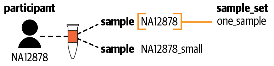
Figure 13-9. The data model—the structure of the example dataset.

Note that having a sample identifier that is identical to a participant identifier normally happens only when there is just one sample per participant. In a realistic research context in which a participant has multiple samples associated with it, you would expect to have different identifiers. You would also expect the two sample datasets to have originated from different biological samples or to have been generated using different assays, whereas we know that in this case they originated from the same one. Again, this is due to the somewhat artificial nature of the example data. In the next step of this scenario, we’re going to look at some data that follows more realistic expectations.

Getting to Know the 1000 Genomes High Coverage Dataset

As we discussed earlier, the Data Library provides access to a collection of datasets hosted by various organizations in several kinds of data repositories. Accordingly, the protocol for retrieving data varies depending on the repository. In this exercise, we retrieve data from a repository that hosts a whole-genome dataset of the 2,504 samples from Phase 3 of the 1000 Genomes Project, which were recently resequenced by the New York Genome Center as part of the AnVIL project. This particular repository simply consists of a public workspace containing only data tables, which serves as a simple but effective form of data repository at this scale.

Go to the 1000 Genomes data workspace now, either by clicking the direct link above or by browsing the Data Library. If you choose the latter route, be aware that there is another 1000 Genomes Project data repository, as shown in Figure 13-10, but it’s quite different: that one contains the Low Coverage sequence data for the full 3,500 study participants, whereas we want the new High Coverage sequence data from the 2,504 participants who were included in Phase 3 of the project.

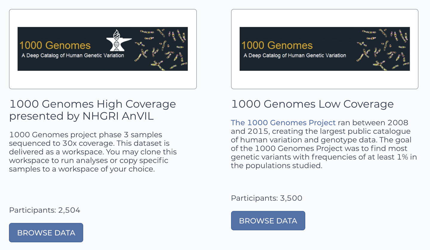
Figure 13-10. The Terra Data Library contains two repositories of data from the 1000 Genomes Project.

When you’re in the workspace, head over to the Data page to check out the data tables. You’ll see the same three tables as we described in the GATK workspace: sample, participant, and sample_set. As expected, the participant table lists the 2,504 participants in the dataset. Similarly, the sample table lists the paths to the location of the corresponding sequence data files, which are provided in CRAM format as well as a GVCF file produced by running a HaplotypeCaller pipeline on the sequence data. In addition, both contain a lot of metadata fields that were not present in the GATK workspace, including information about the data generation stage (type of instrumentation, library preparation protocol, etc.) and the population of origin of the study participant. The presence of all this metadata is a big indicator that this is a more realistic dataset, compared to the toy example data in the GATK workspace. Meanwhile, the sample_set table contains a list of all 2,504 samples associated with the sample set name 1000G-high-coverage-2019-all.

We can summarize the data model for this dataset as follows: each Participant has a single associated Sample, and there is one Sample Set that references all the Samples, as shown in Figure 13-11.

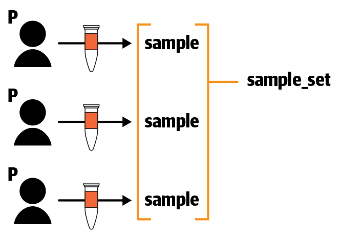
Figure 13-11. The data model for the 1000 Genomes High Coverage dataset.

At this point, we have a confession to make: all this time we’ve spent looking at the data tables of the two workspaces wasn’t mere data tourism. It all had a very specific purpose, to answer the unspoken question that you might or might not have seen coming: will their data models be compatible?

And the good news is yes, they seem to be compatible, meaning that you can combine their data tables without causing a conflict, and you should be able to run a federated data analysis across samples from both datasets. Admittedly the degree of federation here is not really meaningful because only one person’s genomic information is in the GATK workspace, but the underlying principle will apply equally to other datasets that you might want to bring together into a single workspace.

Now that we’re satisfied that we should be able to use the data in our workspace, let’s figure out how to actually perform the transfer of information.

Copying Data Tables from the 1000 Genomes Workspace

There are two main ways to do this: a point-and-click approach, and a load file–based approach. Let’s begin with the point-and-click approach because it abstracts away some of the complexity involved in using load files.

On the Data page of the 1000 Genomes High Coverage workspace, click the sample table and choose a few samples by selecting their corresponding checkboxes on the left. Locate and click the three-dots symbol above the table to open the action menu (as you did in Chapter 11 to configure data inputs for the workflow) and select “Export to Workspace” as shown in Figure 13-12.

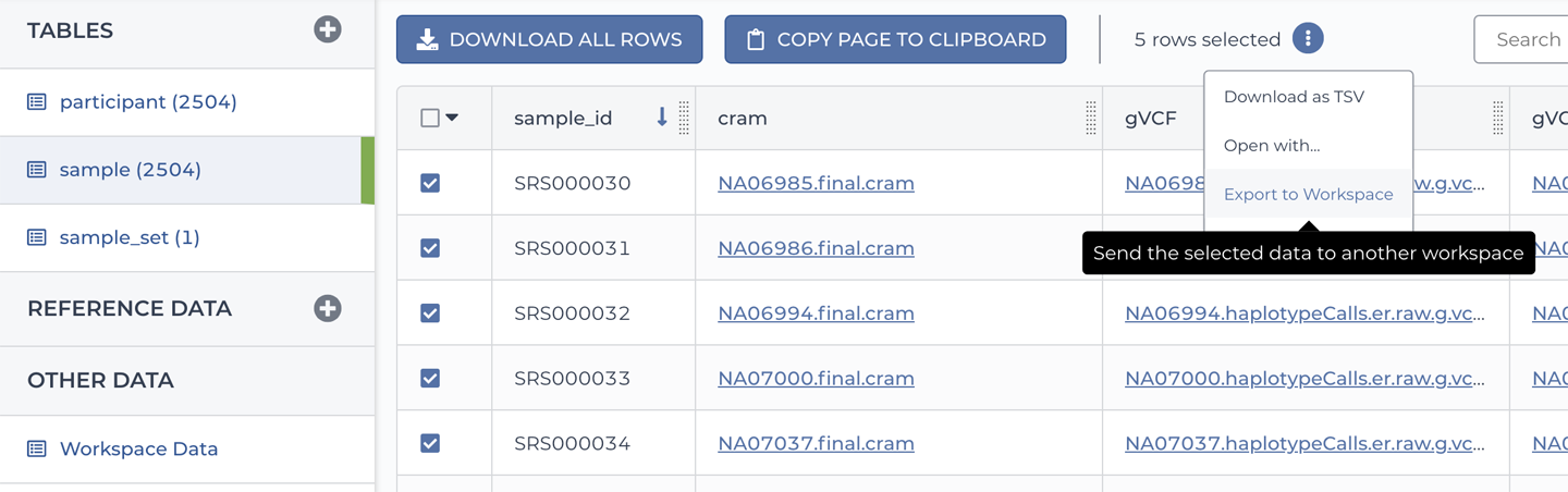
Figure 13-12. The Copy Data to Workspace dialog box.

This should open a dialog box with the list of samples and a workspace selection menu. Select your clone of the GATK workspace and then click Copy. Keep in mind that despite what the buttons seem to imply, we’re not going to copy over any files; we just want to copy over the metadata in the data tables, which include the paths to the locations of the files in GCS. So, rest assured you’re not suddenly going to be on the hook for a big data storage bill.

You should see a confirmation message that asks you whether you want to stay where you are (in the 1000 Genomes workspace) or go to where you copied the data (the GATK workspace). Select the latter option so we can go look at what the transfer produced. If everything worked as expected, you should see the samples you selected listed in the sample table. However, you will not see the corresponding participants listed in the participant table, because the system does not automatically copy over the data from other tables to which the selected data refers. The only exceptions to this are sets, like the sample sets we’ve been working with. If you select a set and copy that over, the system will also copy over the contents of the set. If you also want to copy over the participants, you need to do it as a separate step, either by selecting the rows of interest using the checkboxes or by defining a participant set using a load file.

If you play around with the “copy data to workspace” functionality a little bit, you will quickly realize that this approach is fairly limiting for dealing with large datasets. Why? Because when you try to select all rows in a table, even using the checkbox in the upper-left corner of the table, the system really selects only the items that are displayed on the page. Because the maximum allowed for that is one hundred items, the set approach is your only option for copying over more than one hundred samples at a time using the point-and-click approach.

So now let’s try the load file–based approach, which has some advantages if you are working with large datasets or need to tweak something before copying over the data.

Using TSV Load Files to Import Data from the 1000 Genomes Workspace

Technically, you’ve already done this—that’s how we had you copy over the data table from the original book tutorial workspace to re-create your own earlier in this chapter. You selected the table, clicked the Download All Rows button, retrieved the downloaded file, and then uploaded it to the new workspace. Boom. All our samples are belong to you.

However, this time there’s a twist: several data tables are involved, and some of them have references to the others. As a result, there’s going to be an order of precedence: you must start with the table that doesn’t have any references to the others because Terra can’t handle references to things that it hasn’t seen defined yet. For example, you can’t upload a sample set before having uploaded the samples to which the sample set refers. This is an annoying limitation, and you could imagine having the system simply create a stand-in for any reference to something that it doesn’t recognize. Yet we need to work with the system in its current state, so the bottom line is this: order matters; deal with it.

In practice, for this exercise, you need to download the TSVs for the three data tables from the 1000 Genomes workspace, as previously described (in any order), and then upload them in the correct order to your GATK workspace clone. What is the correct order, you ask? Here’s a hint: look at the visual representation of the data model in Figure 13-11 and use the direction of the arrows to inform your decision. What do you think? That’s right, you first upload the participants, then the samples, and then the sample set. Go ahead and do that now.

Oh wait, did you encounter something you didn’t expect while doing that? Indeed: there are two load files for the sample set: one that defines the table itself and names the sample sets that it contains, identified as entity:sample_set_id, and one that lists the members that each sample set contains, identified as membership:sample_set_id. Have a look at their contents to get a sense of how they relate to each other. And relate they do; because the membership TSV refers to the name of the sample set defined in the entity TSV, you’ll need to upload the entity list first, then the membership list.

Note

Dealing with load files and the precedence rules is one of the more awkward, and frankly tedious, parts of setting up data in Terra. We expect that future developments will address this by providing some kind of wizard-style functionality to smooth out the sharp edges.

On the bright side, after you’re done with that, you should see all 2,504 samples from the 1000 Genomes dataset listed in your GATK workspace as well as their corresponding participants. However, there’s a problem. Can you see it? Take a good look at the columns in the sample table. Most of the columns were different between the two original tables, of course, because the GATK workspace version mainly had output files from the workflows that are showcased in the workspace, and the 1000 Genomes workspace version mainly had metadata about the provenance of the data. However, they were supposed to have one thing in common: GVCF files. Can you find them? Yes, they do all have GVCF files—but they’re in different columns.

In the original GATK workspace, the name of the column containing the GVCF files was gvcf in all lowercase, whereas in the 1000 Genomes workspace it was gVCF in mixed case. Incidentally, the columns containing their respective index files are also named with subtle differences, gvcf_index versus gVCF_TBI, where TBI refers to the extension of the index format generated by a utility called Tabix.

Well, shucks. We were going to surprise you by saying, “Look, now you can run a joint calling analysis of your NA12878 sample combined with all of the 1000 Genomes Phase 3 data. Isn’t that cool?” But it’s not going to work if the GVCF files are in different columns (sad face Emoji).

Chin up; this is fixable. You still have the TSV files that you used to upload the 1000 Genomes data tables, right? Just open the sample TSV file and rename the two columns to match the corresponding names in the GATK workspace. No need to change anything else, just those two column names. Then, upload the TSV and see what happens: now the GVCF files from the 1000 Genomes samples and their index files also show up in the right columns. Crisis averted! The old columns with the mismatching names are still there, but you can ignore them. Literally, in fact; you can hide them (and any others you don’t care about) to reduce the visual clutter. Simply click the gear icon in the upper-right corner of the table to open the table display menu. You can clear the checkboxes for the column names to hide them and even reorder them to suit your preferences.

Note

It’s admittedly a little annoying that you can’t simply edit column names in place or delete unwanted columns. The import dialog box feels a bit limited, as well—we would love to be able to preview the data and get a summary count of rows and columns, for example, before confirming the import operation. We’re looking forward to seeing these aspects of the interface improve as Terra matures.

Fortunately, we were able to get past this trivial little naming mismatch by editing just two column names. However, minor as it might seem, this stumbling block is symptomatic of a much larger problem: there is not enough standardization around how datasets are structured and how their attributes are named. Almost any attempt to federate datasets from different sources can quickly turn into an exercise in frustration as you find yourself battling conflicting schemas and naming conventions. There is no universal solution (yet), but when you encounter this kind of issue, it can be helpful to start by reducing the problem to the smallest set of components that need to be reconciled. For example, try to define the core data model of each dataset; that is, determine the key pieces of data and how they relate to one another. From there, you can gauge what it would take to make the datasets compatible to the extent that you need them to be.

In our case, we now have what we need: all our samples are defined in the sample table and have a GVCF file listed in the gvcf column as well as a corresponding index file in the gvcf_index column. Anything else is irrelevant to what we want to do next, which is to apply joint calling to all the samples in the workspace.

Running a Joint-Calling Analysis on the Federated Dataset

To cap off this scenario, we’re going to run the 3_Joint_Discovery workflow that is preconfigured in this workspace, which applies the GATK Best Practices for joint-calling germline short variants on a cohort of samples as described in Chapter 6. We’re going to run it on a subset of the samples for testing purposes, but we’ll provide pointers for scaling up the analysis in case you want to try running it on all the samples. In any case, the workflow will produce a multisample VCF containing variant calls for the set of samples that we choose to include.

As we admitted earlier, calling this a federated dataset is a bit of an exaggeration given that we’re really adding just one sample to the 1000 Genomes Phase 3 data. However, the principles we’re discussing would apply equally if you were now to add more samples to this workspace. For example, you might want to use the 1000 Genomes data to pad your analysis of a small cohort in order to maximize the benefits you can get from doing joint calling, as is recommended in the GATK documentation.

The workflow is already configured, so let’s have a look at what it expects. Go to the Workflow page and click the 3_Joint_Discovery workflow to view the configuration details. First, we’re going to look at which table the workflow is configured to run on. The data selection drop-down menu shows Sample Set, which means that we’ll need to provide a sample set from the sample_set table. That table currently holds two sample sets; one that lists the NA12878 sample alone, and the other that lists the full 1000 Genomes Phase 3 cohort that we imported into the workspace. We need a sample set that lists some samples from the 1000 Genomes cohort and the NA12878 sample from the GATK workspace, so let’s create one now.

Note

We’re going to use 25 samples because that is how much data the predefined configuration of the workflow can accommodate; we’ll provide guidance for scaling up once we’ve completed the test at this scale.

To quickly create a test sample set, set the data table selector to sample_set under Step 1, and click Select Data under Step 2. In the dialog box that opens up, select the “Create a new set from selected samples” option. You can select the checkboxes of individual samples or select the checkbox at the top of the column to select all 25 samples that are displayed by default. When you’ve selected the samples, you can use the box labeled “Selected samples will be saved as a new set named” to specify a name for the sample set or leave the default autogenerated name as is. Press OK to confirm and return to the workflow configuration page. Note that, at this point, you haven’t actually created the new sample set; you’ve just set up the system to create it when you press the Launch button.

But don’t press the button yet! We want to show you another way to create a sample set, not just because we have a mean streak (we do), but also to equip you to deal with more-complex situations.

The interface for creating sets can be too limiting when you’re working with a lot more samples than can be displayed on a single screen, so we’re also going to show you how to use the manual TSV approach to do this. This is going to be a two-step process, similar to what you did earlier: create a new sample set using an entity load file and then provide a list of its members using a membership load file. The first one is really minimal because it’s just the one column header, entity:sample_set_id, and the name of the new sample set in the next row, as shown here:

entity:sample_set_id

federated-dataset

You can save this as a TSV file and upload it to your workspace as previously, or you can take advantage of the alternative option illustrated in Figure 13-13, which involves copying and pasting the two rows into a text field. Annoyingly, it’s not possible to type text directly into this text box or edit what you paste in, but it does cut out a few clicks from the import process.

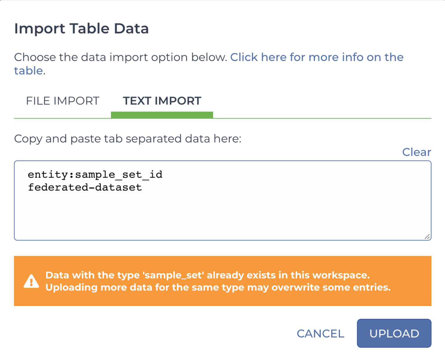
Figure 13-13. Direct text import of TSV-formatted data table content.

Uploading that content creates a new row in the sample_set table, but the new sample set has no samples associated with it yet. To remedy that, we need to make a membership TSV file containing the list of samples that we want to run on. We like to start from existing data tables because it reduces the chance that we’ll get something wrong, especially those finicky header lines. To do so, download the TSV files corresponding to the sample set table and open the sample_set_membership.tsv file in your spreadsheet editor. As shown in Figure 13-14, you should see the full list of 1000 Genomes samples in the second column, with the name of the original 1000 Genomes sample set displayed in the first column of each row. If you scroll all the way to the end of the file, you’ll also see the NA12878 sample from the GATK workspace, which is assigned to the one_sample set.

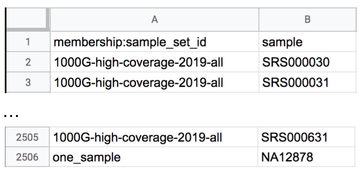
Figure 13-14. Start and end rows of the membership load file sample_set_membership.tsv.

We’re going to take a subset of this and transform it into a membership list that associates the samples we choose with our newly created sample set, federated-dataset. Start by deleting all but 24 of the samples that belong to the 1000 Genomes cohort from the list, so that you’re left with 25 samples in total in the list. It doesn’t matter which samples you keep. Then, use the Find and Replace or Rename function of your editor (typically found on the Edit menu) to change the sample set name in the first column to federated-dataset for all rows, as demonstrated in Figure 13-15. Make sure to also replace the sample set name for the NA12878 sample. Then, save and upload the file as you’ve done previously.

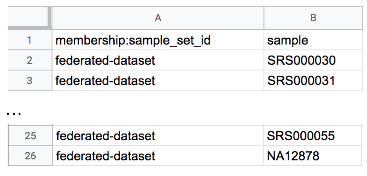
Figure 13-15. Updated membership load file sample_set_membership.tsv assigning 25 samples to the federated-dataset sample set.

After you’ve uploaded this membership list, the sample_set table should now list the 25 samples as belonging to the federated-dataset sample set, as shown in Figure 13-16.

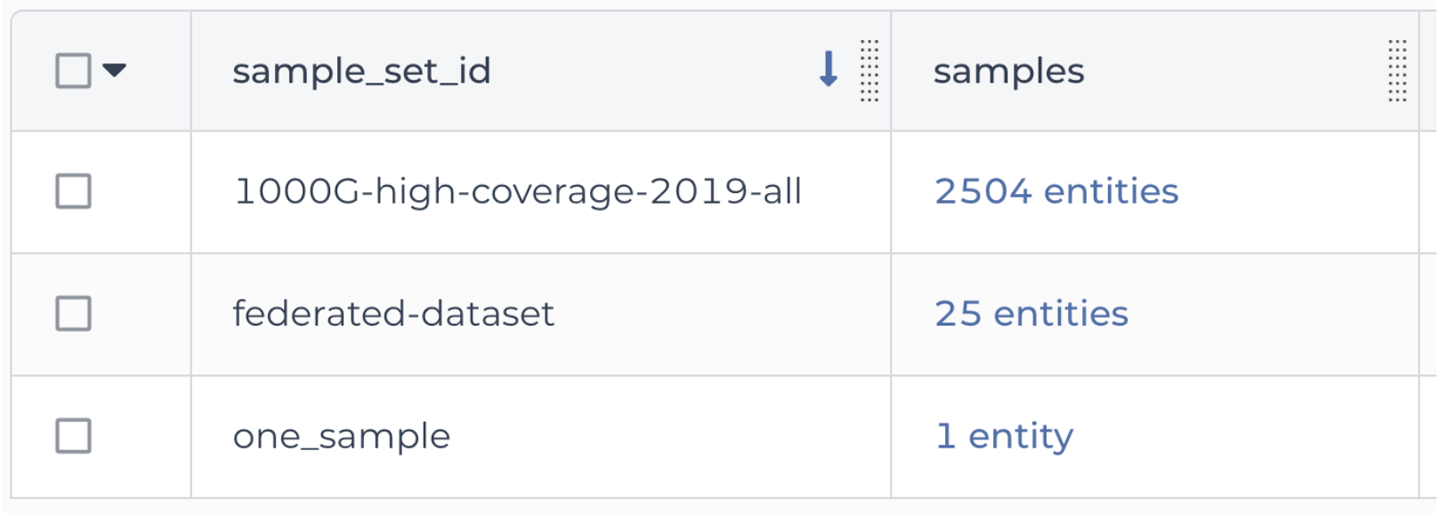
Figure 13-16. The sample_set table showing the three sample sets.

By the way, this shows you that you can add or modify rows by uploading TSV content for just the parts of the table you want to update or augment. You don’t need to reproduce the full table every time. We feel this makes up a bit for not being able to just create the sample sets in the graphical interface.

Note

In case you’re wondering why we’re including only the full-scale NA12878 sample from the GATK workspace and not the downsampled NA12878_small sample, it’s because they come from the same original person so it would be redundant to use both. Because the downsampled one has less data, it’s less likely to produce meaningful results, hence that’s the one we eliminate.

Now that we have a sample set that lists all of the samples that we want to use in our analysis, we can proceed with the next step. Select the checkbox on the left of the federated-dataset row in the sample_set table and then click the “Open with” button, select Workflow, and finally, select 3_Joint_Discovery to initiate the workflow submission. As we’ve shown you previously, you can choose to kick off the process from a selection of data on the Data page like this, or you can do it from the Workflows page, as you prefer. The advantage of doing it as we just described is that now your workflow is already set to run on the right sample set; otherwise, you would need to use the Select Data menu to do it when you get to the configuration page.

At this point, all that remains for us to do is check the remainder of the configuration, starting with the Inputs. There are a lot of input fields so we’re not going to look at all of them; instead, let’s focus on the main file inputs. Based on what you learned about joint calling in Chapter 6, you should have an idea of what kind of input variable you’re looking for: one that refers to a list of GVCFs. Sure enough, if you scroll down a bit, you’ll find the workflow variable named input_gvcfs, as shown in Figure 13-17. The Type of the variable is Array[File], which means the workflow expects us to provide a list of files as input, so that checks out. You also see a corresponding variable set up for the list of index files.

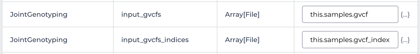
Figure 13-17. Input configuration details for the input_gvcfs and input_gvcfs_indices variables.

Now if you look at the value provided in the rightmost column of the input configuration panel, you see this.samples.gvcf. That should seem both familiar and new at the same time. Familiar because it appears to be a variation of the this.something syntax that we’ve seen and used previously, which allows us to say, “For each row of the table that the workflow runs on, give the content of the something column to this input variable.” We used this previously when launching the HaplotypeCaller workflow on multiple samples for parallel execution; this syntax allowed us to easily wire up the input_bam variable to take the input BAM file for each workflow invocation, without having to specify any files explicitly.

Yet it’s also a bit new because it includes an extra element, forming a this.other.something syntax. Can you guess what’s going on there? This is really cool; it’s the payoff from establishing the connections between tables that we mentioned earlier in the chapter. This syntax is basically saying, “For each sample set, look up the list in its samples column, and then go to the sample table and round up all the GVCF files from the corresponding rows.” You can use this .other. element to refer to any list of rows from another table, query them for a particular field, and return a list of the corresponding elements. And that is how we generate the list of input GVCF files based on the list of samples linked in the sample set. As a bonus, the order in which the list is made is consistent, so we can assign this.samples.gvcf and this.samples.gvcf_index to two different variables, and rest assured that the lists of GVCF files and their index files will be in the same sample order.

This is one of the key benefits of having a well-designed data model in place; you can take advantage of the relationships between data entities at different levels. You can even daisy-chain them several levels deep; there is theoretically no limit to how many .other. lookups you could do. For more examples of what you can do along these lines, check out the data model used in the somatic Best Practices workspaces, where each participant has a tumor sample and a normal sample. In that data model, one additional table lists the Tumor-Normal pairs and another lists sets of pairs.

Feel free to scroll through the rest of the Inputs configuration page. Then, when you feel like you have a good grasp of how the inputs are wired up, head over to the Outputs for one last check before you launch the workflow. The outputs are all set up along a this.output_* pattern, and you should see a line that says, “References to outputs will be written to Tables / sample_set,” which tells you that the final VCF and related output files will be attached to the sample set. This makes sense because by definition the results of a joint calling analysis pertain to all of the samples that are included.

Finally, go ahead and launch the workflow. You can monitor the execution and explore results the same way as in previous exercises. On 25 samples, our test run of the workflow cost $10 and took about 10 hours (with a couple of preemptions) to run to completion. The longest-running step by far was ImportGVCFs, which ran for about three hours per parallelized segment of the genome and spent half that time in the file localization stage. That’s a classic indication that this step would strongly benefit from being optimized to stream data. The other long-running task that is parallelized, GenotypeGVCFs, took about one hour per parallelized segment. Finally, the variant recalibration step, which is not parallelized, took about two hours.

We recommend running this again with a few cohort sizes and comparing the timing diagram for the various runs in order to understand how the time and cost of this workflow scale, depending on the number of samples. You’ll need to create new sample sets by following the same instructions as earlier, but keeping however many samples you’re interested in. Be sure to give each sample set a different name and do the entity TSV step to add it to the table; otherwise, it will just update the sample set you originally created. If you choose to run the workflow on a larger number of samples than the 25 we’ve tested so far, you’ll need to make a few configuration changes according to the instructions in the workspace dashboard, under the 3_Joint_Discovery workflow input requirements. In a nutshell, you’ll need to allocate more disk space to account for the larger number of sample GVCFs that will need to be localized, using the disk override input variables.

The truth of the matter is that this version of the joint discovery workflow suffers from key scaling inefficiencies, including that it does not use streaming, as we pointed out a moment ago, and does not automatically handle resource allocation scaling. We used it for this exercise because it’s conveniently available and fully supported by the GATK support team. Frankly, it’s a great way to observe the consequences of inefficiencies that might seem small individually but would cause substantial difficulties at the scale of thousands of samples. However, we do not recommend attempting to run it on the full cohort—in fact, we wouldn’t advise going above a few hundred samples until you’ve at least run some preliminary scale testing to gauge how the workflow time and cost increase with the number of samples.

If you need something that scales better out of the box, an alternative version of this workflow is supposed to scale better, but as of this writing, it has not gone through the GATK support team’s publishing process, so it is not officially supported. In addition, its input requirements do not allow you to run it directly on the data tables in your workspace because it expects a sample map file that lists sample names and GVCF files as shown in this example (but with multiple lines, one for each sample). To get past this obstacle, you could make such a file based on the sample table in your workspace and add it as a property of the sample set, or if you’re feeling adventurous, you could even write a short WDL task that would run before the main workflow. We leave this as the proverbial exercise for the reader.

This scenario started out with the goal of illustrating a few shortcuts that you can take when assembling a workspace to run GATK Best Practices, but in the process, you also picked up some bonus nuggets of knowledge: what to watch out for when combining data from different origins, how to set up an analysis on the resulting federated dataset, and how a well-crafted data model empowers you to pull together data across different levels. To cap it all off, you ran a complex analysis across a cohort of multiple whole-genome samples without breaking a sweat. Nicely done.

For our last scenario of the chapter, we’re going to flip the order of operations and see how that affects our workspace-building process.

Building a Workspace Around a Dataset

So far, we’ve been taking a very tool-first approach in our scenarios, mainly because our primary focus is on teaching you how to work with a certain range of tools within the cloud computing framework offered by GCP and Terra. Accordingly, our guiding pattern has been to set up tools and then bring in data. However, we recognize that in practice, many of you will follow a data-first approach: bring in data and then figure out how to apply various tools.

In this last scenario, we’re going to walk through an example of what that would look like applied to the same 1000 Genomes dataset that we used in the previous scenario. This time, instead of cloning the GATK workspace and pulling in the 1000 Genomes data from the library, we’re going to clone the 1000 Genomes workspace and pull in a GATK workflow from the public tool repository Dockstore.

Cloning the 1000 Genomes Data Workspace

Navigate back to the 1000 Genomes High Coverage dataset workspace in the Data Library and clone it as you’ve done previously, specifying a name and a billing project. As we discussed at the beginning of this chapter, cloning a workspace makes a shallow copy of its contents, which means that the data files in the bucket will not be copied to the clone. The clone’s data tables will simply point to the original file locations; you can assure yourself that this is true by looking up the file locations in the clone and in the original. This is equivalent to the result of the copy operation we performed in the previous scenario, first by using the data copy option in the interface, and then by repurposing the original workspace’s TSV load files.

Note

In your clone, feel free to replace some or all of the description in the Dashboard with a link to the original to make space for your own notes.

Importing a Workflow from Dockstore

Now the question becomes how do we get some workflows in to analyze this data? As usual in Terra, you have a few options, depending on what you’re trying to achieve. First, you could simply use the internal Methods Repository as you did previously—either put in your own workflow or browse the public section to see if you can find a workflow you like. However, the internal Methods Repository is used only by people who do their work in Terra, so it’s probably missing a lot of interesting workflows that are developed by others in the wider biomedical community.

Another option is to simply copy over a workflow from another workspace; for example, you could grab the 3_Joint_Discovery workflow from the GATK Best Practices workspace (either the original or the clone you used in the previous scenario) by using the “Copy to another workspace” option in the workspace actions menu (circle icon with stacked dots). However, that again limits you to workflows that have already been brought into Terra. In practice, you will likely find some interesting workflows outside of Terra, so we’re going to show you how to import workflows from Dockstore, an increasingly popular registry targeted at the biomedical community that supports workflows written in WDL, CWL, and Nextflow.

Introducing the Dockstore Repository

Dockstore is a public workflow registry developed and operated by the University of California, Santa Cruz, and Ontario Institute for Cancer Research (OICR) intended as a place for workflow authors to publish their workflows for use by the wider community. This is similar to the way code is released on GitHub or a Docker image is published on DockerHub; in fact, Dockstore uses both under the hood. In a nutshell, publishing a workflow in Dockstore consists mainly of linking a GitHub repository where the workflow code resides and providing metadata about the workflow and its inputs. Similarly, registering a container image for a tool involves linking a repository in DockerHub or Quay.io. To learn more about how to publish your own tool containers and workflows in Dockstore, see the extensive online documentation.

In your clone of the 1000 Genomes workspace, navigate to the Workflows page and click the Find a Workflow button, as you’ve done previously. This time, instead of choosing the internal Methods Repository, select the Dockstore option. This takes you to the Dockstore website, where you’ll be able to browse a collection of WDL workflows. On the lefthand menu, you should see a search box that says “Enter search term.” Type joint discovery and view the list of results in the righthand panel (there is no button to press), which will include several GATK workflows, as shown in Figure 13-18.

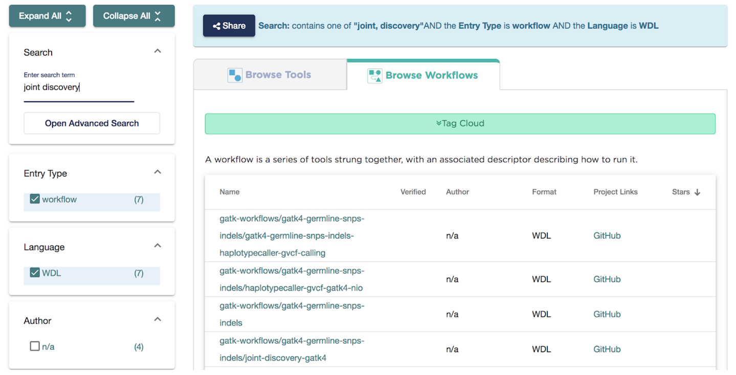
Figure 13-18. Search results for “joint discovery” in Dockstore.

Some of the workflows listed in the results are different versions of the same workflow, registered separately for historical reasons. Unfortunately, the information summarized in the list of search results does not provide a way to easily differentiate between them, so you might sometimes need to click through to the detailed descriptions to understand how they differ.

Find the workflow called gatk-workflows/gatk4-germline-snps-indels/joint-discovery-gatk4 and click through to its detailed information page. This workflow’s name and description should feel at least a little bit familiar because this is actually the source of the 3_Joint_Discovery workflow that you used in the previous scenario. The code itself is in GitHub, in one of the repositories under the gatk-workflows organization used by the GATK support team to publish official GATK workflows. If you click the Versions tab on the workflow details page, you can see a list of code development branches and releases from the GitHub repository. There should be one version tagged as default by the person who registered the workflow, which amounts to them saying, “Unless you know otherwise, this is the version you should use.”

It can sometimes be interesting to look at this to see whether the workflow you’re interested in is under active development; for example, in this case, as of this writing, we see that the default was set to version 1.1.1 in May 2019, yet recent work was done in a development branch as recently as January 2020. Perhaps those changes will have been released by the time you read this, and a new default version will have been set.

You can explore the various other tabs for yourself, but we’d like to point out a couple more that we find especially useful in addition to those we’ve already reviewed. The first is the Files tab, which references the WDL source file under Descriptor Files, and a JSON file of inputs under Test Parameter Files. This is boring now, but it will come in handy later. The other tab we really like is the DAG tab, which stands for directed acyclic graph and refers to the workflow graph. This offers you an interactive visualization of the workflow akin to what you generated with Womtool in Chapter 9, though the display is slightly different, as you can see in Figure 13-19. By default, this just shows tasks in the workflow, which is a pretty neat way to get a high-level view of how the workflow is wired up without looking at the WDL code. There is also an option to switch to a different visualization tool made by a company called EPAM, which provides a much more granular view that includes inputs and outputs. This is very cool for a deep dive, but the amount of detail can be a bit overwhelming.

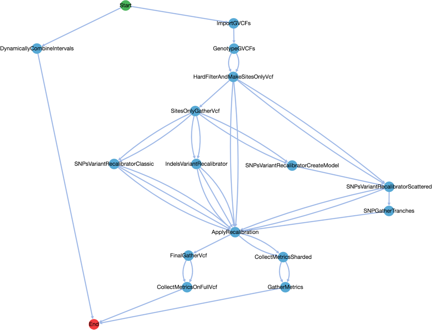
Figure 13-19. The Joint Discovery workflow provided in the DAG tab in Dockstore.

When you’re done exploring the workflow details in the Dockstore interface, look for the box in the right menu labeled “Launch with,” which offers you several options for running the workflow, including Terra. Click the Terra button to return to Terra with the workflow in your pocket. In the import screen that asks you which workspace you want to put it in, select your clone of the 1000 Genomes workspace. You will land on the configuration page of the newly imported workflow in your workspace.

Configuring the Workflow to Use the Data Tables

The Inputs page will be completely bare, so the first thing we recommend doing is uploading the example JSON file of inputs that was listed on the Files tab in Dockstore. Yes, this is why we mentioned that boring tab. Unfortunately, currently there is no way to have Terra import that file along with the workflow itself (obvious feature request right there, folks), so you’ll need to download a copy and then upload it to your workflow configuration using the Upload a JSON option. When the upload is complete, save the configuration and check that there are no remaining error indicators (orange exclamation marks) on the Inputs page. Make sure you select the option to run the workflow directly on file paths and then try running the imported workflow to make sure that everything works out of the box.

Assuming the test run completes successfully, you’re going to need to reconfigure the inputs to point to the data tables instead of direct file paths. This can be the most difficult part of the process, because you must figure out which inputs need to be plugged into the data tables, which ones make sense to move to the workspace resources table, and which one to just leave in the configuration. A good rule of thumb for figuring out the first set is to look at the workflow documentation for a description of its input requirements. There won’t always be one in the workflows you find out in the field, but when there is one, it’s usually highly illuminating with regard to what you should consider to be the main inputs of the workflow. In the case of this particular workflow, you should know what to wire up because we just spent a good chunk of this chapter poking at it, so go do that now. If you get stumped, remember that you can look at the original GATK workspace for a model of what you’re aiming for.

Note

Regarding what’s appropriate to move to the workspace resources table, it’s really just a matter of judgment and preference because there is no real technical difference as far as Terra is concerned. You could simply decide to leave everything in the workflow until you import another workflow and realize they utilize the same resources, and plan to move the relevant resources over to the workspace data table at that time.

When you have the configuration set up, you’ll need to define a sample set by following the same instructions as we gave you in the previous scenario. In fact, at this point, all the remaining work is almost exactly the same as the last two sections of the previous scenario, so we don’t feel the need to walk you through every step again; we’re confident that you can do it on your own. Good luck!

Finally, if you’re feeling a bit short-changed because we made you import the same workflow as in the previous section, here’s a suggestion for a stretch assignment to flex your new muscles on a new-to-you workflow. Sometimes, you might want to redo the GVCF calling step if enough has changed in the algorithms or the supporting resources (e.g., if there is a new reference genome build), but the sequencing data files provided with the 1000 Genomes High Coverage dataset are all in CRAM format, which the GATK team does not yet recommend using for direct data access when using streaming. As a result, you need to find either a CRAM-to-BAM conversion workflow to run as a preprocessing step, or a GATK Haplotype-Caller workflow that starts with a built-in CRAM-to-BAM conversion task. That should ring a bell if you paid attention in Chapter 9.

So go ahead and try finding the appropriate workflow or combination of workflows to achieve that with the 1000 Genomes data, using the various approaches and resources we’ve given you over the past few chapters. If you get really stuck, let us know by posting an issue in the GitHub repository, and we’ll help you work through it. If a lot of people report difficulties with the stretch assignments, we’ll consider posting step-by-step solutions in the blog.

Wrap-Up and Next Steps

In this chapter, you learned how to assemble your own workspace in Terra from data and code components originating from various sources, both internal and external to Terra. We put a lot of emphasis on thinking about how datasets are structured in order to empower you to take advantage of the power of linked data tables in Terra and to combine data from different sources in general. You practiced importing data from the Data Library and running a federated analysis that included data from the 1000 Genomes Project, setting the stage for large-scale analyses. You also learned to import workflows from Dockstore, a tool and workflow repository that can connect to several other platforms besides Terra. At this point, you have all the necessary foundations to be able to assemble and execute your own scalable analysis from publicly or privately available tools and datasets on the cloud. In Chapter 14, the final chapter, we walk through an example of a workspace that reproduces an end-to-end analysis from a published paper to illustrate current capabilities, obstacles, and perspectives for achieving optimal computational reproducibility in biomedical research.