Chapter 3. Computing Technology Basics for Life Scientists
In an ideal world, you wouldn’t need to worry too much about computing infrastructure when you’re pursuing your research. In fact, in later chapters we introduce you to systems that are specifically designed to abstract away the nitty-gritty of computing infrastructure in order to help you focus on your science. However, you will find that a certain amount of terminology and concepts are unavoidable in the real world. Investing some effort into learning them will help you to plan and execute your work more efficiently, address performance challenges, and achieve larger scale with less effort. In this chapter, we review the essential components that form the most common types of computing infrastructure, and we discuss how their strengths and limitations inform our strategies for getting work done efficiently at scale. We also go over key concepts such as parallel computing and pipelining, which are essential in genomics because of the need for automation and reproducibility. Finally, we introduce virtualization and lay out the case for cloud infrastructure.
The first few sections in this chapter are aimed at readers who have not had much training, if any, in informatics, programming, or systems administration. If you are a computational scientist or an IT professional, feel free to skip ahead until you encounter something that you don’t already know. The last two sections, which together cover pipelining, virtualization, and the cloud, are more specifically focused on the problems that we tackle in this book and should be informative for all readers regardless of background.
Basic Infrastructure Components and Performance Bottlenecks
Don’t worry; we’re not going to make you sit through an exhaustive inventory of computer parts. Rather, we’ve put together a short list of the components, terminology, and concepts that you’re most likely to encounter in the course of your work. In relation to each of these, we’ve summarized the main performance challenges and the strategies that you might need to consider to use them effectively.
Let’s begin with a brief overview of the types of processors that you might come across in scientific computing today.
Types of Processor Hardware: CPU, GPU, TPU, FPGA, OMG
At its simplest, a processor is a component in your computer that performs computations. There are various types of processors, with the most common being the central processing unit (CPU) that serves as the main processor in general-use computers, including personal computers such as laptops. The CPU in your laptop may have multiple cores, subunits that can process operations more or less independently.
In addition to a CPU, your personal computer also has a graphical processing unit (GPU) that processes the graphical information for display on your screen. GPUs came into the limelight with the development of modern video games, which require extremely fast processing to ensure smooth visual rendering of game action. In essence, the GPU solution outsources the rather specific type of processing involved in mathematical calculations like matrix and vector operations from the CPU to a secondary processing unit that specializes in handling certain types of calculations that are applied to graphical data very efficiently. As a result, GPUs are also becoming a popular option for certain types of scientific computing applications that involve a lot of matrix or vector operations.
The third type of processor you should know about is called a field-programmable gate array (FPGA), which, despite breaking with the *PU naming convention, is also a type of processing unit; however, it’s unlikely that you’ll find one in your laptop. What’s interesting about FPGAs is that unlike GPUs, FPGAs were not developed for a specific type of application; quite the contrary, they were developed to be adaptable for custom types of computations. Hence “field-programmable” as part of their name.
On GCP, you might also come across something called a tensor processing unit (TPU), which is a kind of processor developed and branded by Google for machine learning applications that involve tensor data. A tensor is a mathematical concept used to represent and manipulate multiple layers of data related to vectors and matrices. Consider that a vector is a tensor with one dimension, and a matrix is a tensor with two dimensions; more generally, tensors can have arbitrary numbers of dimensions beyond that, so they are very popular in machine learning applications. TPUs belong to a category of processors called application-specific integrated circuit (ASIC), which are custom designed for specialized uses rather than general use.
Now that you have the basic types of processors down, let’s talk about how they are organized in typical high-performance computing setups.
Levels of Compute Organization: Core, Node, Cluster, and Cloud
When you move beyond personal computers and into the world of high-performance computing, you’ll hear people talk about cores, nodes, and either clusters or clouds, as illustrated in Figure 3-1. Let’s review what these mean and how they relate to one another.
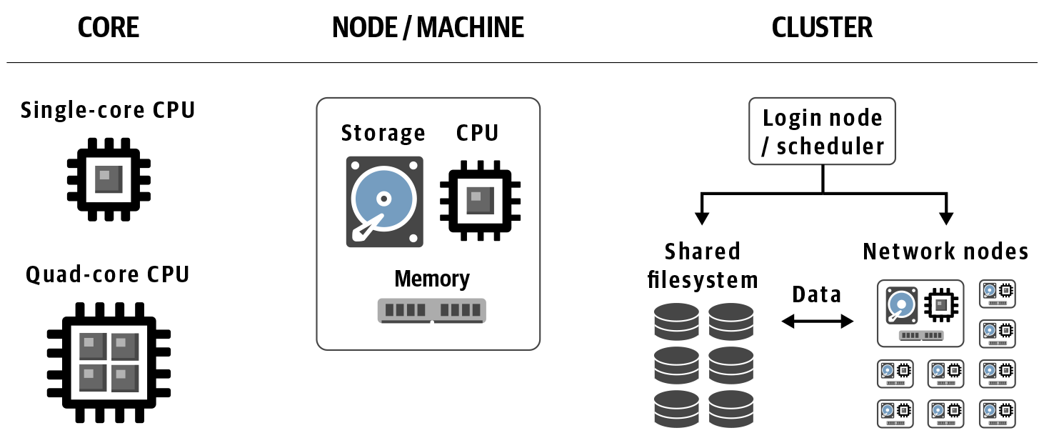
Figure 3-1. Levels of compute organization.
Low level: core
A core is the smallest indivisible processing unit within a machine’s, or node’s, processor unit, which can comprise one or more cores. If your laptop or desktop is relatively recent, its CPU probably has at least two cores, and is therefore called dual-core. If it has four, it’s a quad-core, and so on. High-end consumer machines can have more than that; for example, the latest Mac Pro has a twelve-core CPU (which should be called dodeca-core if we follow the Latin terminology) but the CPUs on professional-grade machines can have tens or hundreds of cores, and GPUs typically have an order of magnitude more, into the thousands. Meanwhile, TPUs have core counts in the single digits like consumer CPUs, and FPGAs break the mold entirely: their cores are defined by how they are programmed, not by how they are built.
Mid level: node/machine
A node is really just a computer that is part of a cluster or cloud. It is analogous to the laptop or desktop computer that most of us interact with primarily in our day-to-day work, except without the dedicated monitor and peripherals we are used to seeing associated with personal computers. A node is also sometimes simply called a machine.
Top level: cluster and cloud
A cluster and a cloud are both a collection of machines/nodes.
A cluster is an HPC structure composed of nodes networked together to some extent. If you have access to a cluster, the chances are that either it belongs to your institution, or your company is renting time on it. A cluster can also be called a server farm or a load-sharing facility.
A cloud is different from a cluster in that in its resting state, its nodes are not explicitly networked together. Rather, it is a collection of independent machines that are available to be networked (or not) depending on your needs. We cover that in more detail in the final section of this chapter, along with the concept of virtualization, which gives us virtual machines (VMs), and containerization, which gives us Docker containers.
For now, however, we move on to the very common concern of how to use a given set of computing infrastructure effectively, which typically revolves around identifying and solving key computational bottlenecks. As with the rest of this chapter, an in-depth exploration of this topic would be beyond the scope of this book, so we’re aiming simply to familiarize you with the key concepts and terminology.
Addressing Performance Bottlenecks
You’ll occasionally find that some computing operations seem slow and you’ll need to figure out how to make them go faster (if possible). The solutions available to you will depend on the nature of the bottleneck you’re facing.
At a very high level, following are the main operations that the computer typically has to perform (not necessarily in a linear order):
-
Read some data into memory from the permanent storage where it resides at rest
-
Have the processor execute instructions, transforming data and producing results
-
Write results back to the permanent storage
Data storage and I/O operations: hard drive versus solid state
Steps 1 and 3 are called I/O operations (I/O stands for input/output). You might hear people describe some software programs as being “I/O-bound,” which means the part of the program that takes the longest is reading and writing data to and from relatively slow storage. This is typically the case for simple programs that do things like file format conversions, in which you’re just reading in some data and writing it out in a different shape, and you’re not doing any real computing (i.e., there’s little to no math involved). In those cases, you can speed up operation by using faster storage drives; for example, solid-state drives (SSDs) rather than hard-disk drives (HDDs). The key difference between them is that HDDs have physical disks called platters that spin and an armature that reads data from and writes it to the platter via magnetics—like a tiny high-tech turntable—whereas SSDs have no moving parts. That makes SSDs less prone to physical malfunctions and also quite a bit faster at accessing data.
If you’re working with a networked infrastructure in which the storage drives are not directly connected to the computing nodes, you will also be limited by the speed at which data can be transferred over the network connections. That can be determined by hardware factors as pedestrian as the kind of cables used to connect the network parts. Although you might not notice the difference when computing on small files, you definitely will notice it when running on whole genomes; and even on a network with very fast transfer speeds, transferring whole genomes will consume some noticeable time.
Memory: cache or crash
Step 2 is where your program is taking data and applying some kind of transformation or calculation, aka the interesting part. For a lot of applications, the calculation requires holding a lot of information in memory. In those cases, if your machine doesn’t have enough memory, it might resort to caching, which is a way of using local storage space as a substitute for real memory. That allows you to keep working, but now your processes become I/O bound because they need to copy data back and forth to slow storage, which takes you back to the first bottleneck. In extreme cases, the program can stall indefinitely, fail to complete, or crash. Sometimes, it’s possible for a developer to rewrite the program to be smarter about the information it needs to see concurrently, but when it’s not, the solution is to simply add more memory. Fortunately, unlike memory in humans, computer memory is just hardware, and it comes relatively cheap.
Specialized hardware and code optimizations: navigating the trade-offs
At times, the nature of the program requires the processor itself to do a lot of heavy lifting. For example, in the widely used GATK tool HaplotypeCaller, an operation can calculate genotype likelihoods; we need to compute the likelihood of every single sequence read given each candidate allele using a hidden Markov model (HMM) called PairHMM (don’t worry if this sounds like gibberish at the moment—it’s just a bunch of genomics-specific math). In some areas of the genome, that leads us to do millions of computations per site across a very large number of sites. We know from performance profiling tests, which record how much time is spent in processing for each operation in the program, that PairHMM is by far the biggest bottleneck for this tool. We can reduce this bottleneck in some surface-level ways; for example, by making the program skip some of the computations for cases in which we can predict they will be unnecessary on uninformative. After all, the fastest way to calculate something is to not calculate it at all.
Being lazy gets us only so far, however, so to get to the next level, we need to think about the kind of processor we can (or should) use for the work we need to do. Not just because some processors run faster than others, but also because it’s possible to write program instructions in a way that is very specific to a particular type and architecture of processor. If done well, the program will be extra efficient in that context and therefore run faster. That is what we call code optimization, and more specifically native code optimization because it must be written in a low-level language that the processor understands “natively” without going through additional translation layers.
Within a type of processor like CPUs, different manufacturers (e.g., Intel and AMD) develop different architectures for different generations of their products (e.g., Intel Skylake and Haswell), and these different architectures provide opportunities for optimizing the software. For example, the GATK package includes several code modules corresponding to alternative implementations of the PairHMM algorithm that are optimized for specific Intel processor architectures. The program automatically activates the most appropriate version when it finds itself running on Intel processors, which provides some useful speed gains.
However, the benefits of hardware optimizations are most obvious across processor types; for example, if you compare how certain algorithms perform when implemented to run on FPGAs instead of CPUs. The Illumina DRAGEN toolkit (originally developed by Edico Genome) includes implementations of tools like HaplotypeCaller that are optimized to run on FPGAs and as a result are much faster than the original Java software version.
The downside of hardware-optimized implementations is that by definition, they require specialized hardware. This can be a big problem for the many research labs that rely on shared institutional computing systems and don’t have access to other hardware. In contrast, applications written in Java, like GATK, can run on a wide range of hardware architectures because the Java Virtual Machine (JVM) translates the application code (called bytecode in the Java world) into instructions appropriate for the machine. This separation of concerns (SoC) between the bytecode of Java and what actually is executed on the machine is called an abstraction layer and it’s incredibly convenient for everyone involved. Developers don’t need to worry about exactly what kind of processor we have in our laptops, and we don’t need to worry about what kind of processor they had in mind when they wrote the code. It also guarantees that the software can be readily deployed on standard off-the-shelf hardware, which makes it usable by anyone in the world.
Sometimes, you’ll need to choose between different implementations of the same algorithms depending on what is most important to you, including how much you prize speed over portability and interoperability. Other times, you’ll be able to enjoy the best of both worlds. For example, the GATK team at the Broad Institute has entered into a collaboration with the DRAGEN team at Illumina, and the two teams are now working together to produce unified DRAGEN-GATK pipelines that will be available both as a free open source version (via Broad) and as a licensed hardware-accelerated version (via Illumina). A key goal of the collaboration is to make the two implementations functionally equivalent—meaning that you could run either version and get the same results within a margin of error considered to be insignificant. This will benefit the research community immensely in that it will be possible to combine samples analyzed by either pipeline into downstream analyses without having to worry about batch effects, which we discussed briefly in the previous chapter.
Parallel Computing
When you can’t go faster, go parallel. In the context of computing, parallel computing, or parallelism, is a way to make a program finish sooner by performing several operations in parallel rather than sequentially (i.e., waiting for each operation to finish before starting the next one). Imagine that you need to cook rice for 64 people, but your rice cooker can make enough rice for only 4 people at a time. If you need to cook all of the batches of rice sequentially, it’s going to take all night. But if you have eight rice cookers that you can use in parallel, you can finish up to eight times sooner.
This is a simple idea but it has a key requirement: you must be able to break the job into smaller tasks that can be performed independently. It’s easy enough to divide portions of rice because rice itself is a collection of discrete units. But you can’t always make that kind of division: for example, it takes one pregnant woman nine months to grow a baby, but you can’t do it in one month by having nine women share the work.
The good news is that most genomic analyses are more like rice than like babies—they essentially consist of a series of many small independent operations that can be parallelized. So how do we get from cooking rice to executing programs?
Parallelizing a Simple Analysis
Consider that when you run an analysis program, you’re just telling the computer to execute a set of instructions. Suppose that we have a text file and we want to count the number of lines in it. The set of instructions to do this can be as simple as this:
Open the file; count the number of lines in it; tell us the number; close the file.
Note that “tell us the number” can mean writing it to the console or storing it somewhere for use later on—let’s not worry about that right now.
Now suppose that we want to know the number of words on each line. The set of instructions would be as follows:
Open the file; read the first line; count the number of words; tell us the number; read the second line; count the number of words; tell us the number; read the third line; count the number of words; tell us the number.
And so on until we’ve read all the lines, and then finally we can close the file. It’s pretty straightforward, but if our file has a lot of lines, it will take a long time, and it will probably not use all the computing power we have available. So, to parallelize this program and save time, we just cut up this set of instructions into separate subsets, like this:
-
Open the file; index the lines.
-
Read the first line; count the number of words; tell us the number.
-
Read the second line; count the number of words; tell us the number.
-
Read the third line; count the number of words; tell us the number.
-
[Repeat for all lines.]
-
Collect final results and close the file.
Here, the “read the Nth line” steps can be performed in parallel because they are all independent operations.
You’ll notice that we added a step, “index the lines.” That’s a little bit of preliminary work that allows us to perform the “read the Nth line” steps in parallel (or in any order we want) because it tells us how many lines there are and, importantly, where to find each one within the file. It makes the entire process much more efficient. As you will see in the following chapters, tools like GATK require index files for the main data files (reference genome, read data and variant calls). The reason is to have that indexing step already done so that we can have the program look up specific chunks of data by their position in the genome.
Anyway, that’s the general principle: you transform your linear set of instructions into several subsets of instructions. There’s usually one subset that has to be run first and one that has to be run last, but all the subsets in the middle can be run at the same time (in parallel) or in whatever order you want.
From Cores to Clusters and Clouds: Many Levels of Parallelism
So how do we go from rice cookers to parallelizing the execution of a genomic analysis program? Overall, the action of parallelizing computing operations consists of sending subsets of the work we want done to multiple cores for processing. We can do that by splitting up the work across the cores of a single multicore machine, or we can dispatch work to other machines if we have access to a cluster or cloud. In fact, we can combine the two ideas and dispatch work to multicore machines, in which the work is further split up among each machine’s cores. Going back to the rice-cooking example, it’s as if instead of cooking the rice yourself, you hired a catering company to do it for you. The company assigns the work to several people, who each have their own cooking station with multiple rice cookers. Now, you can feed a lot more people in the same amount of time! And you don’t even need to clean the dishes.
Whether we want to distribute the work across multiple cores on a single machine or across multiple machines, we’re going to need a system that splits up the work, dispatches jobs for execution, monitors them for completion, and then compiles the results. Several kinds of systems can do that, falling broadly into two categories: internal or external to the analysis program itself. In the first case, the parallelization happens “inside” the program that we’re running: we run that program’s command line, and the parallelization happens without any additional “wrapping” on our part. We call that multithreading. In the second case, we need to use a separate program to run multiple instances of the program’s command line. An example of an external parallelization is writing a script that runs a given tool separately on the data from each chromosome in a genome and then combines the result with an additional merge step. We call that approach scatter-gather. We cover that in more detail in the next section when we introduce workflow management systems. In Figure 3-2, you can see how we can use multithreading and scatter-gather parallelism in the course of an analysis.
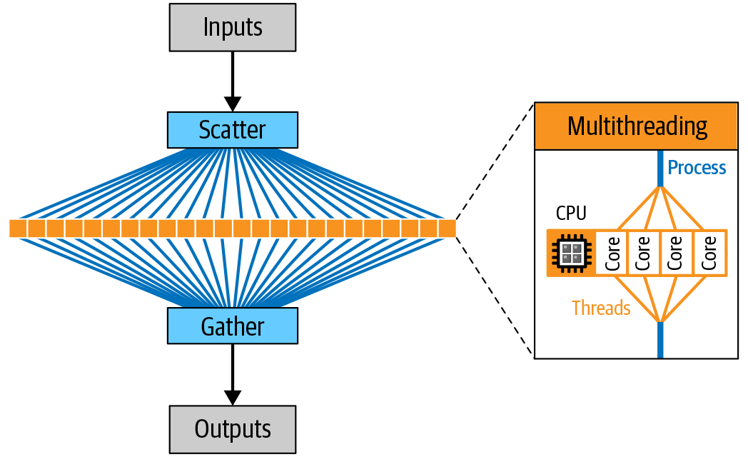
Figure 3-2. Scatter-gather allows parallel execution of tasks on different CPU cores (on a single machine or multiple machines, depending on how it’s implemented).
Trade-Offs of Parallelism: Speed, Efficiency, and Cost
Parallelism is a great way to speed up processing on large amounts of data, but it has overhead costs. Without getting too technical at this point, let’s just say that parallelized jobs need to be managed, you need to set aside memory for them, regulate file access, collect results, and so on. So it’s important to balance the costs against the benefits, and avoid dividing the overall work into too many small jobs. Going back to our earlier example, you wouldn’t want to use a thousand tiny rice cookers that each boil a single grain of rice. They would take far too much space on your countertop, and the time required to distribute each grain and then collect it when it’s cooked would more than negate any benefits from parallelizing in the first place.
More generally, although it’s tempting to think of parallelism as a way to make things go faster, it’s important to remember that the impression of speed is entirely subjective to the observer. In reality, the computation being run on each piece of data is not going any faster. We’re just running more computations at the same time, and we’re limited by the parallel capacity of our computing setup (typically measured in number of nodes or cores) as well as hardware limitations like I/O and network speeds. It’s more realistic to think of parallelism as a way to optimize available resources in order to finish tasks sooner, rather than making individual tasks run faster.
This distinction might seem pedantic given that, from the point of view of the human at the keyboard, the elapsed time (often called wall-clock time; that is, “the time shown by the clock on the wall”) is shorter. And isn’t that what we all understand as going faster? However, from the point of view of the resources we utilize, if we add up the time spent doing computation by the processor across all the cores we use, we might find that the overall job takes more time to complete compared to purely sequential execution because of the overhead costs.
That brings us to another important question: what is the monetary cost of utilizing those resources? If we’re working with a dedicated machine that is just sitting there with multiple cores and nothing else to do, the parallelization is still absolutely worth it, even with the overhead. We’ll want to parallelize the heck out of everything we do on that machine in order to maximize efficiency. However, when we start working in the cloud environment, as we do in Chapter 4, and we need to start paying for itemized resources as we go, we’ll want to look more carefully at the trade-offs between minimizing wall-clock time and the size of the bill.
Pipelining for Parallelization and Automation
Many genomic analyses involve running a lot of routine data-processing operations that need to be parallelized for efficiency and automated to reduce human error. We do this by describing the workflow in a machine-readable language, which we then can feed into a workflow management system for execution. We go over how this works in practice in Chapter 8, but first let’s set the stage by introducing basic concepts, definitions, and key software components. As we go, please keep in mind that this field currently has no such thing as a one-size-fits-all solution, and it’s ultimately up to you to review your needs and available options before picking a particular option. However, we can identify general principles to guide your selection, and we demonstrate these principles in action using the open source pipelining solution that is recommended by the GATK development team and used in production at the Broad Institute. As with most of this book, the goal here is not to prescribe the use of specific software, but to show through working examples how all of this fits together in practice.
One tricky aspect is that we have dozens of scripting languages and workflow management systems to choose from in the bioinformatics world—likely hundreds if you look at a wider range of fields. It can be difficult to compare them directly because they tend to be developed with a particular type of audience in mind, leading to very different modalities of user experience. They are often tuned for particular use cases and are sometimes optimized to operate on certain classes of infrastructure. We often see one solution that is preferred by one group prove to be particularly difficult or frustrating to use for another. These various solutions are also generally not interoperable, meaning that you can’t take a workflow script written for one workflow management system and run it unmodified on the next one over. This lack of standardization is a topic of both humor and desperation in just about every field of research known to humankind, as is illustrated in Figure 3-3.
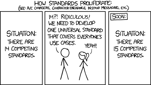
Figure 3-3. XKCD comic on the proliferation of standards (source: https://xkcd.com/927).
In recent years, we have seen some high-profile initiatives such as the Global Alliance GA4GH emerge with the explicit mission of developing common standards and consolidating efforts around a subset of solutions that have interoperability as a core value. For example, the GA4GH Cloud Work Stream has converged on a small set of workflow languages for its driver projects, including CWL, Nextflow, and WDL, which we use in this book. At the same time, given the recognition that no single language is likely to satisfy all needs and preferences, several groups are working to increase interoperability by building support for multiple workflow languages into their workflow management systems. The workflow management system we use in this book, Cromwell, supports both WDL and CWL, and it could be extended to support additional languages in the future.
Workflow Languages
In principle, we could write our workflows in almost any programming language we like; but in practice, some are more amenable than others for describing workflows. Just like natural languages, programming languages also exhibit a fascinating diversity and can be classified in various ways including grammar, mode of execution, and the programming paradigms that they support.
From a practical standpoint, we begin by making a distinction between all-purpose programming languages, which are intended to be usable for a wide range of applications, and domain-specific languages (DSLs) that are, as the name indicates, specifically designed for a particular domain or activity. The latter are typically preloaded with things like specially formulated data structures (i.e., ways to represent and manipulate data that “understand” the nature of the underlying information) and convenience functions that act as shortcuts; for example, handling domain-specific file formats, applying common processing actions, and so on. As a result, a DSL can be an attractive option if your needs fit well within the intended scope of the language, especially if your computational background is limited, given that the DSL typically enables you to get your work done without having to learn a lot of programming concepts and syntax.
On the other hand, if your needs are more varied or you are used to having the more expansive toolbox of a general-purpose language at your disposal, you might find yourself uncomfortably constrained by the DSL. In that case, you might prefer to use a general-purpose language, especially one enriched with domain-specific libraries that provide relevant data structures and convenience functions (e.g., Python with Biopython and related libraries). In fact, using a general-purpose language is more likely to enable you to use the same language for writing the data-processing tasks themselves and for managing the flow of operations, which is how many have traditionally done this kind of work. What we’re seeing now in the field, however, is a move toward separation of description and content, which manifests as increased adoption of DSLs specifically designed to describe workflows as well as of specialized workflow management systems. This evolution is strongly associated with the push for interoperability and portability.
Popular Pipelining Languages for Genomics
When we look at the cross-section of people who find themselves at the intersection of bioinformatics and genomics, we see a wide range of backgrounds, computational experience, and needs. Some come from a software engineering background and prefer languages that are full featured and highly structured, offering great power at the cost of accessibility. Some come from systems administration and believe every problem can be solved with judicious application of Bash, sed, and awk, the duct tape of the Unix-verse. On the “bio” side of the fence, the more computationally trained tend to feel most at home with analyst favorites like Python and R, which have been gaining ground over old-time classics Perl and MATLAB; some also tend to gravitate toward DSLs. Meanwhile wetlab-trained researchers might find themselves baffled by all of this, on initial contact at least. (Author’s note and disclaimer: Geraldine identifies as one of the initially baffled, having trained as a traditional microbiologist and eventually learned the rudiments of Perl and Python in a desperate bid to escape the wetlab workbench. Spoiler: it worked!)
Based on recent polling, some of the languages that are most popular with workflow authors in the genomics space are SnakeMake and Nextflow. Both are noted for their high degree of flexibility and ease of use. Likewise, CWL and WDL are picking up steam because of their focus on portability and computational reproducibility. Of the two, CWL is more frequently preferred by people who have a technical background and enjoy its high level of abstraction and expressiveness. In contrast, WDL is generally considered to be more accessible to a wide audience.
At the end of the day, when it comes to picking a workflow language, we look at four main criteria: what kind of data structures the language supports (i.e., how we can represent and pass around information), how it enables us to control the flow of operations, how accessible it is to read and write for the intended audience, and how it affects our ability to collaborate with others. Whatever we choose, it’s unlikely that we can satisfy everyone’s requirements. However, if we were to boil all this down to just one recommendation, it would be this: if you want your workflow scripts to be widely used and understood in your area of research, pick a language that is open and accessible enough to newcomers yet scales well enough to the ambitions of the more advanced. And, of course, try to pick a language that you can run across different workflow management systems and computing platforms, because you never know what environment you or your collaborators might find yourselves in next.
Workflow Management Systems
Many workflow management systems exist, but in general they follow the same basic pattern. First, the workflow engine reads and interprets the instructions laid out in the workflow script, translating the instruction calls into executable jobs that are associated with a list of inputs (including data and parameters). It then sends out each job with its list of inputs to another program, generally called a job scheduler, that is responsible for orchestrating the actual execution of the work on the designated computing environment. Finally, it retrieves any outputs produced when the job is done. Most workflow management systems have some built-in logic for controlling the flow of execution; that is, the order in which they dispatch jobs for execution and for determining how they deal with errors and communicate with the compute infrastructure.
Another important advance for increasing portability and interoperability of analyses is the adoption of container technology, which we cover in detail in the last section of this chapter. For now, assume that a container is a mechanism that allows you to encapsulate all software requirements for a particular task, from the deepest levels of the operating system (OS) all the way to library imports, environment variables, and accessory configuration files.
Virtualization and the Cloud
Up to this point, we have been assuming that whether you’re working with a single computer or a cluster, you’re dealing with “real” physical machines that are each set up with a given OS and software stack, as represented in Figure 3-4 A. Unfortunately, interacting with that kind of system has several disadvantages, especially in a shared environment like an institutional cluster. As an end user, you typically don’t have a choice regarding the OS, environment, and installed software packages. If you need to use something that isn’t available, you can ask an administrator to install it, but they might decline your request or the package you want might not be compatible with existing software. For the system administrators on the other side of the helpdesk, it can be a headache to keep track of what users want, manage versions, and deal with compatibility issues. Such systems take effort to update and scale.
That is why most modern systems use various degrees of virtualization, which is basically a clever bit of abstraction that makes it possible to run multiple different software configurations on top of the same hardware through virtual machines (VMs) and containers as represented in Figure 3-4 B and C respectively. These constructs can be utilized in many contexts, including optionally on local systems (you can even use containers on your laptop!), but they are absolutely essential for cloud infrastructure.
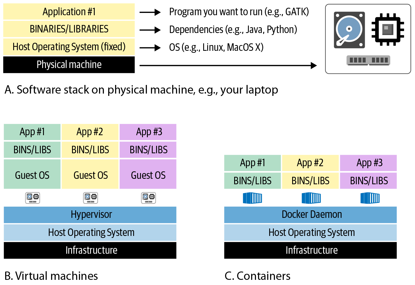
Figure 3-4. A) The software stack installed on a physical machine; B) a system hosting multiple VMs; C) a system hosting multiple containers.
VMs and Containers
A VM is an infrastructure-level construct that includes its own OS. The VM sits on top of a virtualization layer that runs on the actual OS of the underlying physical machine(s). In the simplest case, VMs can be run on a single physical machine, with the effect of turning that physical machine into multiple servers that share the underlying resources. However, the most robust systems utilize multiple physical machines to support the layer of VMs, with a complex layer between them that manages the allocation of physical resources. The good news is that for end users, this should not make any difference—all you need to know is that you can interact with a particular VM in isolation without worrying about what it’s sitting on.
A container is similar in principle to a VM, but it is an application-level construct that is much lighter and more mobile, meaning that it can be deployed easily to different sites, whereas VMs are typically tied to a particular location’s infrastructure. Containers are intended to bundle all the software required to run a particular program or set of programs. This makes it a lot easier to reproduce the same analysis on any infrastructure that supports running the container, from your laptop to a cloud platform, without having to go through the pain of identifying and installing all the software dependencies involved. You can even have multiple containers running on the same machine, so you can easily switch between different environments if you need to run programs that have incompatible system requirements.
If you’re thinking, “These both sound great; which one should I use?” here’s some good news: you can use both in combination, as illustrated in Figure 3-5.

Figure 3-5. A system with three VMs: the one on the left is running two containers, serving App #1 and App #2; the middle is running a single container, serving App #3; the right is serving App #4 directly (no container).
There are several registries for sharing and obtaining containers, including Docker Hub, Quay.io, and GCR, Google’s general-purpose container registry in GCP. In the registry, the container is packaged as an image. Note that this has nothing to do with pictures; here the word image is used in the same software-specific way that refers to a special type of file. You know how sometimes when you need to install new software on your computer, the download file is called a disk image? That’s because the file you download is in a format that your OS is going to treat as if it were a physical disk on your machine. This is basically the same thing. To use a container, you first tell the Docker program to download, or pull, a container image file from a registry—for example, Docker Hub (more on Docker shortly)—and then you tell it to initialize the container, which is conceptually equivalent to booting up a VM. And after the container is running, you can run any software within it that is installed on its system. You can also install additional packages or perform additional configurations as needed. Figure 3-6 illustrates the relationship between container, image, and registry.
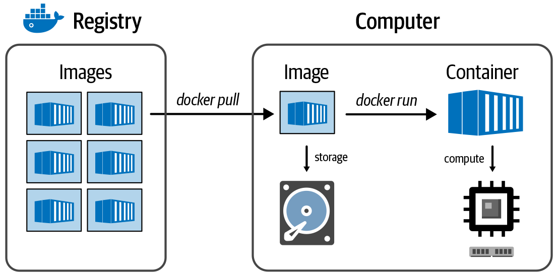
Figure 3-6. The relationship between registry, image, and container.
The most widely used brand of container systems is Docker, produced by the company of the same name. As a result of Docker’s ubiquitousness, people will often say “a docker” instead of “a container,” much like when “xerox” became a replacement for “copy machines” (in the US at least) because of the dominance of the Xerox company. However, docker with a lowercase d is also the command-line program that you install on your machine to run Docker containers. Similarly, although the action of bundling a software tool, package, or analysis into a Docker container should rightly be called “containerizing,” people often call it “dockerizing,” as in, “I dockerized my Python script.” Dockerizing a tool involves writing a script called a Dockerfile that describes all installations and environment configurations necessary to build the Docker image, as demonstrated in Figure 3-7.
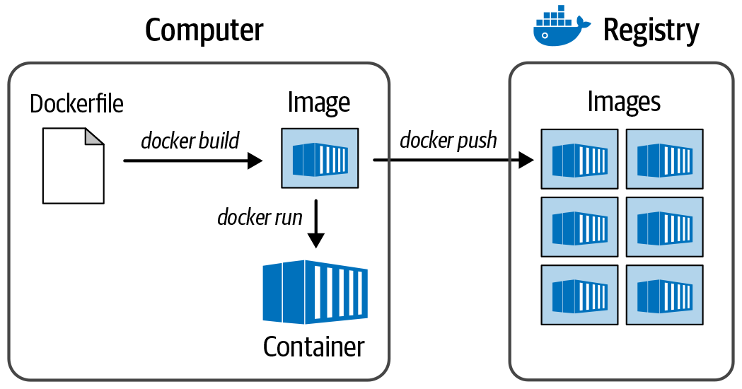
Figure 3-7. The process for creating a Docker image.
As noted earlier, it is possible to use containers in various contexts, including local machines, HPC, and the cloud. One important restriction is that Docker specifically is usually not allowed in shared environments like most institutions’ HPCs, because it requires a very high level of access permissions called root. In that kind of setting, system administrators will prefer Singularity, an alternative system that achieves the same results. Fortunately, it is possible to run Docker containers within a Singularity system.
Introducing the Cloud
Finally, we get to the topic many of you have been waiting for: what is this cloud thing anyway? The surprisingly easy answer is that the cloud is a bunch of computers that you can rent. In practice, that means that as a user, you can easily launch a VM and select how much RAM, storage, and what CPUs you want. You want a VM with 1 TB of RAM and 32 CPUs for genome assembly? No problem! Most of the VMs in the cloud are running some form of Linux as the OS, which you get to choose when you launch it, and are typically accessed using a remote shell via Secure Shell (SSH).
Although some VMs include free storage, this is typically ephemeral and will go away when you stop and start your VM. Instead, use block storage (a persistent device) to store data, scripts, and so on on your VM. You can think of these very much like a USB thumb drive that you can have “plugged” into your VM whenever you like. Even when you terminate your VM, files on block storage will be OK and safely saved. Files can also be stored in object store—think of this more like Google Drive or Dropbox, where files can be read and written by multiple VMs at the same time, but you don’t typically use these as a normal filesystem. Instead, they are more akin to an SSH File Transfer Protocol (SFTP) server for sharing files between VMs, where you transfer files through a utility to and from the object storage system. The final basic component of a cloud is networking. With a virtual networking service, you can control who has access to your VMs, locking it down tightly to ensure that only you (or others you trust) have access.
Clouds are not fluffy
When you think about clouds, they are fluffy, distant, and elusive, not at all concrete, real things that you can touch, feel, and capture. Unlike their namesake, the cloud infrastructure that most of us use directly (or indirectly) today ultimately is composed of real, physical computers racked up and blinking away in huge datacenters. What makes it different, though, from previous models for compute (and rings true to their name) is its ephemeral nature. Just like clouds coming and going—popping up, dumping their rain, and then blowing away—cloud computing is transient for the end user. The cloud allows you as a researcher, developer, or analyst to request computational infrastructure when you need it, to use it for computing as long as you need it, and then you can release all the resources when you’re done.
This approach is great because it saves time and money insomuch as you can spin up a lot of resources at once, get your work done, and spin these back down, saving on the costs or running hardware continuously. You don’t need to think too much about where the servers are racked, how they are configured, the health of the hardware, power consumption, or myriad other infrastructure concerns. These are all abstracted away from you and are taken care of without you having to think about it too much. What you focus on, instead, is the computational work that you need to perform, the resources you need to do it, and how to most effectively use these resources both from a time and money perspective.
Evolution of cloud infrastructure and services
Amazon launched the first widely successful commercial public cloud service in 2006, but the basic idea has been around for a long time. Mainframes in the 1960s were often rented for use, which made a ton of sense, given the massive costs of buying and operating them. Regardless of the invention of the personal computer, the idea of renting computing infrastructure has cropped up again over and over in the intervening decades. In academic groups and industry, the concept of shared grid computing in the 1990s and 2000s was the more modern equivalent of rented mainframe time. Groups banded together to build cheap but powerful Linux-based HPC clusters that were often centrally managed and allocated out to multiple groups based on some sort of financial split.
Today’s public clouds are different, though, in the level of abstraction. Hence, the adoption of the fluffy, amorphous name to reflect the fact that an understanding of the underlying details is not required in order to run large-scale analysis on clouds. When working with a given cloud, you might know the general region of the world that hosts your infrastructure (e.g., North Virginia for AWS us-east-1), but many of the details are hidden from you: how many people are using the underlying hardware of your VM, where the datacenter is really located, how the network is set up, and so on. What you do know are key details that affect service cost and job execution time, like how many CPUs are available, how much RAM the VM has, the uptime guarantees of the file storage system, and the regulations the system conforms to.
There are now many public cloud providers—clouds available to anyone who can pay for the service. The most dominant currently in the Western hemisphere are AWS, Microsoft Azure, and GCP. Each provides a similar mix of services that range from simple VMs rentable by the hour (or minute), file storage services, and networking to more specialized services such as Google’s Cloud TPU service, which allows you to perform accelerated machine learning operations. The important feature, though, is that these resources are provided as services: you use what you need per hour, minute, second, or API call, and are charged accordingly.
Pros and cons of the cloud
One of the major advantages that many people point to when discussing the cloud is cost. When building a datacenter, the fixed costs are enormous. You must hire people to rack and maintain physical servers, monitor the network for intrusion, deal with power fluctuations, backups, air conditioning, and so on. Honestly, it is a lot of work! For a datacenter that supports hundreds of users, the costs associated with maintaining the infrastructure can be worth it. But many researchers, developers, analysts, and others are realizing that they don’t need to have hundreds of computers always available and running, just waiting for a task. Instead, it makes a lot more sense to use a cloud environment in which you can do local work on your laptop, without extensive resources, and then, when your analysis is ready, you can scale up to hundreds or thousands of machines. Commercial public clouds allow you to easily burst your capacity and do a huge analysis when you need to, as opposed to waiting weeks, months, or even years for a dedicated local cluster to finish your tasks. Likewise, you don’t need to pay for the maintenance of local infrastructure for all the time you spend developing your algorithms and perfecting your analysis locally.
Finally, as a public cloud user, you have full control of your environment. Need a specific version of Python? Do you have a funky library that compiles only if very specific tool chains are installed? No problem! The cloud lets you have full control over your VMs, something that a shared, local infrastructure would never allow. Even with this control, when they are set up following cloud vendor best practices, public cloud solutions are invariably more secure than on-premises infrastructure because of the vast amount of resources dedicated to security services in these environments and the isolation between users afforded by virtualization.
Although the public cloud platforms are amazing, powerful, flexible and, in many cases, can be used effectively to save a ton of money in the long run, there are some disadvantages to look out for. If you are looking to always process a fixed number of genomes produced by your sequencing group per month, the public cloud might be less attractive and it would make more sense to build a small local compute environment for this very predictable workload of data produced locally. This is assuming, of course, that you have IT professionals who can act as administrators. Another consideration is expertise. Using the cloud demands a certain level of expertise, and an unsuspecting novice user might accidentally use VMs with weak passwords, set up data storage buckets with weak security, share credentials in an insecure way, or just be totally lost in the process of managing a fleet of Linux VMs. Even these potential downfalls, though, are generally outweighed by the benefits of working flexibly on commercial cloud environments for many people.
Categories of Research Use Cases for Cloud Services
The basic components of the cloud described in the previous section are really just the tip of the iceberg. Many more services are available on the main commercial cloud platforms. In fact, there are far too many services, some universal and some unique to a particular cloud, than we can describe here. But let’s take a look at how researchers might use the services or the cloud most commonly. Table 3-1 provides an overall summary.
| Usage type | Cloud environment | Description | Positives | Negatives |
|---|---|---|---|---|
| Lightweight development | Google Cloud Shell | Using a simple-to-launch free VM for editing code and scripts |
|
|
| Intermediate analysis and development | Single VM | Launching a single VM, logging in, performing development and analysis work |
|
|
| Batch analysis | Multiple VMs via batch system | Using a system like AWS Batch or Google Cloud Pipelines API to launch many VMs and analyze data in parallel |
|
|
| Framework analysis | Multiple VMs via a framework | Using Spark, Hadoop, or other framework for data analysis |
|
|
Lightweight development: Google Cloud Shell
The cloud is a fantastic place for software development. Even though many researchers will want to use their own laptops or workstation for development, there can be some really compelling reasons for using the cloud as a primary development environment, especially for testing. On GCP, for example, you can use the Google Cloud Shell from the Google Cloud Console for light development and testing. This is a free (yes, free!) VM with one virtual CPU core and 5 GB of storage that you can use just by clicking the terminal icon in the web console. This is a fantastic environment for some light coding and testing; just remember to copy code off of your free instance (using Git, for example) because there are quotas for total runtime per week, and, if you don’t use the service for a while, your 5 GB volume might get cleaned out. Still, this is a great option for quickly getting started with the cloud and performing lightweight tasks. You just need a web browser, and the GCP tools are all preinstalled and configured for you. Many other tools that you might want to work with are already installed as well, including Git and Docker, along with languages like Java and Python. You’ll have a chance to try it out early on in the next chapter.
Intermediate development and analysis: single VM
Although the Google Cloud Shell is great for many purposes, easy to use, and free, sometimes you might need a bit more power, especially if you want to test your code or analysis at the next scale up, so you spin up your own dedicated VM. This is perhaps the most commonly used option because of the mix of flexibility and simplicity it offers: you can customize your VM, ensuring you have enough CPU cores, RAM, and local storage to accomplish your goal. Unlike the Google Cloud Shell, you must pay for each hour or minute you run this VM; however, you have full control over the nature of the VM. You might use this for software or algorithm development, testing your analysis approach, or spinning up a small fleet of these VMs to perform analysis on multiple VMs simultaneously. Keep in mind, however, that if you are manually launching these VMs, fewer tools will be preinstalled on them and ready to go for you. That makes using utilities such as Git and Docker very helpful for moving your analysis tasks from VM to VM. You’ll have a chance to use this extensively in Chapter 4 through Chapter 7.
Batch analysis: multiple VMs via batch services
This approach is really the sweet spot for most users who are aware of it. Although you might use your laptop or Google Cloud Shell for software and script development, and one or more VMs for testing them on appropriately sized hardware, you ultimately don’t want to manually manage VMs if your goal is to scale up your analysis. Imaging running 10,000 genome alignments at the same time; you need systems that can batch up the work, provision VMs automatically for you, and turn the VMs off when your work is done. Batch systems are designed just for this task; Google Cloud, for example, offers the Google Cloud Pipelines API, which you can use to submit a large batch of multiple jobs simultaneously. The service will take care of spinning up numerous VMs to perform your analysis and then automatically clean them up after collecting the output files. This is extremely convenient if you need to perform noninteractive analysis on a ton of samples. You’ll see in Chapter 8 through Chapter 11 that workflow engines like Cromwell are designed to take advantage of these batch services, which take care of all the details of launching batch jobs. That makes it much easier for you to focus on the details of the analysis you’re performing rather than on the infrastructure involved.
Framework analysis: multiple VMs via framework services
The final approach that many researchers will use involves interactive, iterative analysis. In genomics, you can use a batch system to perform large-scale alignment and variant calling but, after you have VCF files for your variants, you might choose to move to a Spark cluster, RStudio, Jupyter Notebook, or any of a large number of analytical environments for subsequent analysis. In Chapter 12, we explore how this works in Terra, which you can use to easily create a custom environment for data processing with a Jupyter interface for interactive analysis, generating plots for your publications, and sharing results with others.
Wrap-Up and Next Steps
In this chapter, we completed the primer topics, which gave you a background on genomics (Chapter 2) and computing technologies (this chapter). We delved into the nitty-gritty details of computer hardware, parallel computing, and virtualization and gave you a glimpse of the power of using workflow execution systems to scale out your analysis on the cloud. In Chapter 4, we take our first baby steps to the cloud environment and show you how to get started with your own VMs running in GCP.